Lecture 1 (The Monte Carlo principle) - Institute for Particle Physics ...

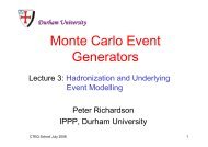
MC techniques Quadratures Monte Carlo Simulation SummaryTopics of the lectures1 Lecture 1: The Monte Carlo Principle2 Lecture 2: Parton level event generation3 Lecture 3: Dressing the Partons4 Lecture 4: Modelling beyond Perturbation TheoryThanks to- My fellow MC authors, especially S.Gieseke, K.Hamilton, L.Lonnblad, F.Maltoni, M.Mangano,P.Richardson, M.Seymour, T.Sjostrand, B.Webber.- the other Sherpas: J.Archibald, S.Höche, S.Schumann, F.Siegert, M.Schönherr, J.Winter, and K.Zapp.F. Krauss IPPPIntroduction to Event Generators

MC techniques Quadratures Monte Carlo Simulation SummaryMenu of lecture 1Prelude: Selecting from a distributionStandard textbook numerical integration (quadratures)Monte Carlo integrationA basic simulation exampleF. Krauss IPPPIntroduction to Event Generators

MC techniques Quadratures Monte Carlo Simulation SummaryPrelude: Selecting from a distributionThe problemA typical Monte Carlo/simulation problem:Distribution of “usual” random numbers #:“flat” in [0, 1].But: Want random numbers x ∈ [x min , x max ],distributed according to (probability) density f(x).F. Krauss IPPPIntroduction to Event Generators

MC techniques Quadratures Monte Carlo Simulation SummaryThe exact solutionThe first method applies if both the integral of the densityf(x) and its inverse are known (i.e. practically never).To see how it works realise that thediff. probability P(x ∈ [x ′ ,x ′ +dx ′ ]) = f(x ′ )dx ′ .Therefore: x given by∫ xx∫maxdx ′ f(x ′ ) = # dx ′ f(x ′ ).x min x minSince everything known:x = F −1 [F(x min )+#(F(x max )−F(x min ))].F. Krauss IPPPIntroduction to Event Generators

MC techniques Quadratures Monte Carlo Simulation SummaryThe work-around solution: “Hit-or-miss”(Solution, if exact case does not work.)Builds on “over-estimator” g(x) (G and G −1 known):g(x) > f(x) ∀x ∈ [x min , x max ].Select an x according to g(with exact algorithm);Accept with probability f(x)/g(x)(with another random number);Obvious fall-back choice for g(x):g(x) = Max [xmin ,x max]{f(x)}.F. Krauss IPPPIntroduction to Event Generators

MC techniques Quadratures Monte Carlo Simulation SummaryQuadratures: standard numerical integrationReminder: Basic techniquesTypical problem: Need to evaluate an integral, cannot doit in closed form.Example: nonlinear pendulum.Can calculate period T from E.o.M. ¨θ = −g/l sinθ:T =√8lgθ∫max0dθ√ cosθ −cosθmaxElliptic integral, no closed solution known=⇒ entering (again) the realm of numerical solutions.F. Krauss IPPPIntroduction to Event Generators

MC techniques Quadratures Monte Carlo Simulation SummaryNumerical integration: Newton-Cotes methodNomenclature now: Want to evaluate I (a,b) ∫ bf= dxf(x).aBasic idea: Divide interval [a,b] in N subintervals of size∆x = (b −a)/N and approximateI (a,b)f=∫ badxf(x)≈ N−1 ∑f(x i )∆x = N−1 ∑f(a+i∆x)∆x,i=0i=0i.e. replace integration by sum over rectangular panels.Obvious issue: What is the error? How does it scaleparametrically with “step-size” (or, better, number offunction calls)? Answer: It is linear in ∆x.F. Krauss IPPPIntroduction to Event Generators

MC techniques Quadratures Monte Carlo Simulation SummaryImproving on the error: Trapezoid, Simpson and allthatA careful error estimate suggests that by replacingrectangles with trapezoids the error can be reduced toquadratic in ∆x.This boils down to including a term [f(b)−f(a)]/2:I (a,b)f≈ N−1 ∑f(x i )∆x + ∆x [f(a)+f(b)] 2i=1Repeating the error-reducing exercise replaces thetrapezoids by parabola: The Simpson rule. In so doing,the error decreases to (∆x) 4 .F. Krauss IPPPIntroduction to Event Generators

MC techniques Quadratures Monte Carlo Simulation SummaryNumerical integration: ResultsConsider test function f(x) = √ 4−x 2 in [0,2].(I (0,2)f2∫= dx √ 4 − x 2 = π).0F. Krauss IPPPIntroduction to Event Generators

MC techniques Quadratures Monte Carlo Simulation SummaryConvergence of numerical integration: SummaryFirst observation: Numerical integrations only yieldestimators of the integral, with an estimated accuracygiven by the error.(Proviso: the function is sufficiently well behaved.)Scaling behaviour of the error translates into scalingbehaviour for the number of function calls necessary toachieve a certain precision.In one dimension/per dimension, therefore, theconvergence scales likeTrapezium rule: ≃ 1/N 2Simpson’s rule ≃ 1/N 4with the number N of function calls.F. Krauss IPPPIntroduction to Event Generators

MC techniques Quadratures Monte Carlo Simulation SummaryMonte Carlo integrationThe underlying idea: Determination of πUse random number generator!F. Krauss IPPPIntroduction to Event Generators

MC techniques Quadratures Monte Carlo Simulation SummaryDetermination of πF. Krauss IPPPIntroduction to Event Generators

MC techniques Quadratures Monte Carlo Simulation SummaryError estimate in Monte Carlo integrationMC integration: Estimate integral by N probesI (a,b)f=∫ b−→ 〈I (a,b)f〉 = b−aNadxf(x)N∑f(x i ) = 〈f〉 a,b ,i=1where x i homogeneously distributed in [a, b]Basic idea for error estimate: statistical sample=⇒ use standard deviation as error estimate〈E (a,b)f(N)〉 = σ =[ 〈f] 2 〉 a,b −〈f〉 1/2. 2a,bIndependent of the number of integration dimensions!=⇒ Method of choice for high-dimensional integrals.NF. Krauss IPPPIntroduction to Event Generators

MC techniques Quadratures Monte Carlo Simulation SummaryDetermination of π: ErrorsF. Krauss IPPPIntroduction to Event Generators

MC techniques Quadratures Monte Carlo Simulation SummaryImprove convergence: Importance samplingWant to minimise number of function calls.(They are potentially CPU-expensive.)=⇒ Need to improve convergence of MC integration.First basic idea: Samples in regions, where f largest( =⇒ corresponds to a Jacobian transformation of integral.)Algorithm:Assume a function g(x) similar to f(x).Obviously f(x)/g(x) is smooth =⇒ 〈E(f/g)〉 is small.Must sample according to dx g(x) rather than dx:g(x) plays role of probability distribution; we knowalready how to deal with this!Works, if f(x) is well-known. Hard to generalise.F. Krauss IPPPIntroduction to Event Generators

MC techniques Quadratures Monte Carlo Simulation SummaryImportance sampling: Example resultsConsider f(x) = cos πx2 and g(x) = 1−x2 :F. Krauss IPPPIntroduction to Event Generators

MC techniques Quadratures Monte Carlo Simulation SummaryImprove convergence: Stratified samplingWant to minimise number of function calls.(They are potentially CPU-expensive.)=⇒ Need to improve convergence of MC integration.Basic idea here: Decompose integral in M sub-integrals∑〈I(f)〉 = M ∑〈I j (f)〉, 〈E(f)〉 2 = M 〈E j (f)〉 2j=1j=1Then: Overall variance smallest, if “equally distributed”.(=⇒ Sample, where the fluctuations are.)Algorithm:Divide interval in bins (variable bin-size or weight);adjust such that variance identical in all bins.F. Krauss IPPPIntroduction to Event Generators

MC techniques Quadratures Monte Carlo Simulation SummaryStratified sampling: Example resultsConsider f(x) = cos πx2 and g(x) = 1−x2 :〈I〉 = 0.637±0.147/ √ NF. Krauss IPPPIntroduction to Event Generators

MC techniques Quadratures Monte Carlo Simulation SummaryExample for stratified sampling: VEGASGood for Vegas:Singularity “parallel” tointegration axesBad for Vegas:Singularity forms ridgealong integration axesF. Krauss IPPPIntroduction to Event Generators

MC techniques Quadratures Monte Carlo Simulation SummaryImprove convergence: Multichannel samplingWant to minimise number of function calls.(They are potentially CPU-expensive.)=⇒ Need to improve convergence of MC integration.Basic idea: Best of both worlds:Hybrid between importance andstratified sampling.Have “bins” – weight α i – of“eigenfunctions” – g i (x):=⇒ g(⃗x) = ∑ Ni=1 α ig i (⃗x).In particle physics, this is the method of choice for partonlevel event generation!F. Krauss IPPPIntroduction to Event Generators

MC techniques Quadratures Monte Carlo Simulation SummaryBasic simulation paradigmAn example from thermodynamicsConsider two-dimensional Ising model:H = −J ∑ s i s j〈ij〉Traditional model to understand (spontaneous)magnetisation & phase transitions.(Spins fixed on 2-D lattice with nearest neighbour interactions.)To evaluate an observable O, sum over all microstatesφ {i} ,givenbytheindividualspins. (SimilartopathintegralinQFT.)〈O〉 = ∫ { [ ]}Dφ {i} Tr O(φ {i} ) exp− H(φ {i})k B TTypical problem in such calculations (integrations!):Phase space too large =⇒ need to sample.F. Krauss IPPPIntroduction to Event Generators

MC techniques Quadratures Monte Carlo Simulation SummaryMetropolis-AlgorithmMetropolis algorithm simulates the canonical ensemble,summing/integrating over micro-states with MC method.Necessary ingredient: Interactions among spins inprobabilistic language(will come back to us.)Algorithm will look like: Go over the spins, check whetherthey flip (compare P flip with random number), repeat toequilibrate.To calculate P flip : Use energy of the two micro-states(before and after flip) and Boltzmann factors.While running, evaluate observables directly and takethermal average (average over many steps).F. Krauss IPPPIntroduction to Event Generators

MC techniques Quadratures Monte Carlo Simulation SummaryWhy Metropolis is correct: Detailed balanceConsider one spin flip, connecting micro-states 1 and 2.Rate of transitions given by the transition probabilities W( )If E 1 > E 2 then W 1→2 = 1 and W 2→1 = exp− E 1−E 2k B TIn thermal equilibrium, both transitions equally often:P 2 W 2→1 = P 1 W 1→2This takes into account that the respective states areoccupied according to their Boltzmann factors.(P i ∼ exp(−E i /k B T))In principle, all systems in thermal equilibrium can bestudied with Metropolis - just need to write transitionprobabilities in accordance with detailed balance, as above=⇒ general simulation strategy in thermodynamics.F. Krauss IPPPIntroduction to Event Generators

MC techniques Quadratures Monte Carlo Simulation SummarySome example resultsFix temperature, use a 10×10 latticeF. Krauss IPPPIntroduction to Event Generators

MC techniques Quadratures Monte Carlo Simulation SummarySummary of lecture 1Discussed some basic numerical techniques.Introduced Monte Carlo integration as the method ofchoice for high-dimensional integration space (phasespace).Introduced some standard improvement strategies to theconvergence of Monte Carlo integration.Discussed connections between simulations and MonteCarlo integration with the example of the Ising model.F. Krauss IPPPIntroduction to Event Generators