Chapter 7. Hypothesis Testing with One Sample

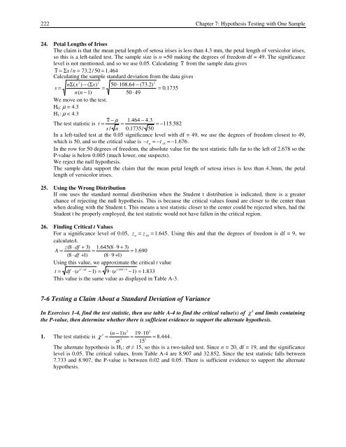
222 Chapter 7: Hypothesis Testing with One Sample24. Petal Lengths of IrisesThe claim is that the mean petal length of setosa irises is less than 4.3 mm, the petal length of versicolor irises,so this is a left-tailed test. The sample size is n =50 making the degrees of freedom df = 49. The significancelevel is not mentioned, and so we use 0.05. Calculating x from the sample data givesx = Σx /n = 73.2 /50 = 1.464Calculating the sample standard deviation from the data givess = nΣ(x 2 ) − (Σx) 250 ⋅108.64 − (73.2)2= = 0.1735n(n −1)50 ⋅ 49We move on to the test.H 0 : µ = 4.3H 1 : µ < 4.3The test statistic is t = x − µ 1.464 − 4.3=s / n 0.1735/ 50 =−115.582In a left-tailed test at the 0.05 significance level with df = 49, we use the degrees of freedom closest to 49,which is 50, and so the critical value is −t α=−t .05=−1.676.In the row for 50 degrees of freedom, the absolute value for the test statistic falls far to the left of 2.678 so theP-value is below 0.005 (much lower, one suspects).We reject the null hypothesis.The sample data support the claim that the mean petal length of setosa irises is less than 4.3mm, the petallength of versicolor irises.25. Using the Wrong DistributionIf one uses the standard normal distribution when the Student t distribution is indicated, there is a greaterchance of rejecting the null hypothesis. This is because the critical values found are closer to the center thanwhen dealing with the Student t. This means a test statistic closer to the center could be rejected when, had theStudent t be properly employed, the test statistic would not have fallen in the critical region.26. Finding Critical t ValuesFor a significance level of 0.05, z α= z .05= 1.645. Using this and that the degrees of freedom is df = 9, wecalculateA.z(8 ⋅ df + 3) 1.645(8 ⋅ 9 + 3)A = = = 1.690(8 ⋅ df +1) (8 ⋅ 9 +1)Using this value, we approximate the critical t valuet = df ⋅ (e A 2 / df−1) = 9 ⋅ (e 1.6902 /9−1) = 1.833This value is the same value as displayed in Table A-3.7-6 Testing a Claim About a Standard Deviation of VarianceIn Exercises 1-4, find the test statistic, then use table A-4 to find the critical value(s) of χ 2 and limits containingthe P-value, then determine whether there is sufficient evidence to support the alternate hypothesis.(n1. The test statistic is χ 2 −1)s2=σ 219 ⋅102= = 8.444.15 2The alternate hypothesis is H 1 : σ ≠ 15, so this is a two-tailed test. Since n = 20, df = 19, and the significancelevel is 0.05. The critical values, from Table A-4 are 8.907 and 32.852. Since the test statistic falls between7.733 and 8.907, the P-value is between 0.02 and 0.05. There is sufficient evidence to support the alternatehypothesis.