lecture notes on matrice and least squares

76 CHAPTER 3 A LITTLE MORE LINEAR ALGEBRAFor example,AB =On the other hand, note well thatBA =0 12 31 23 4 0 12 3 1 23 4==4 78 153 411 16. (3.2.21)= AB. (3.2.22)This definition of matrix-matrix product even extends to the case in which both matricesare vectors. If x ∈ R m and y ∈ R n , then xy (called the “outer” product and usuallywritten as xy T ) is(xy) ij = x i y j . (3.2.23)So ifandthenxy T =x =y =−11⎡⎢⎣130⎤−1 −3 01 3 0(3.2.24)⎥⎦ (3.2.25). (3.2.26)Here is a brief summary of the notation for inner products:x · y = x T y = (x y) = ix i y i = x i y i summation convention3.3 Some Special MatricesThe identity element in the space of square n × n matrices is a matrix with ones on themain diagonal and zeros everywhere else⎡⎤1 0 0 0 . . .0 1 0 0 . . .I n =0 0 1 0 . . .. (3.3.1)⎢. ⎣ . .. ⎥⎦0 . . . 0 0 1

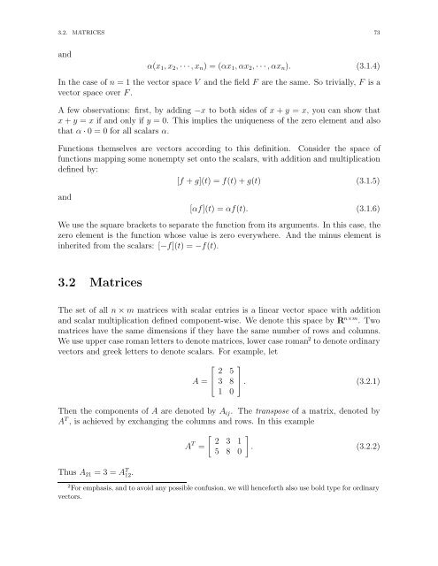
78 CHAPTER 3 A LITTLE MORE LINEAR ALGEBRAthat it is never negative and it is zero if and only if the scalar itself is zero. For vectorsand matrices both we can define a generalization of this concept of length called a norm.A norm is a function from the space of vectors onto the scalars, denoted by · satisfyingthe following properties for any two vectors v and u and any scalar α:Definition 2 NormsN1: v > 0 for any v = 0 and v = 0 ⇔ v = 0N2: αv = |α|vN3: v + u ≤ v + uProperty N3 is called the triangle inequality.The most useful class of norms for vectors in R n is the p norm defined for p ≥ 1 by n 1/px p = |x i | p . (3.4.1)i=1For p = 2 this is just the ordinary Euclidean norm: x 2 = √ x T x. A finite limit of the p norm exists as p → ∞ called the ∞ norm:x ∞ = max1≤i≤n |x i| (3.4.2)We won’t need matrix norms in this class, but in case you’re interested any norm onvectors in R n induces a norm on matrices viaA = maxx=0Axx . (3.4.3)E.g., Let x = (1 1), then x = √ 1 · 1 + 1 · 1 = √ 2.3.5 Projecting Vectors Onto Other VectorsFigure 3.1 illustrates the basic idea of projecting one vector onto another. We can alwaysrepresent one, say b, in terms of its components parallel and perpendicular to the other.The length of the component of b along a is b cos θ which is also b T a/aNow suppose we want to construct a vector in the direction of a but whose length is thecomponent of b along b. We did this, in effect, when we computed the tangential force

3.5. PROJECTING VECTORS ONTO OTHER VECTORS 79yba - bb cos axFigure 3.1: Let a and b be any two vectors. We can always represent one, say b, in termsof its components parallel and perpendicular to the other. The length of the componentof b along a is b cos θ which is also b T a/a.of gravity on a simple pendulum. What we need to do is multiply b cos θ by a unitvector in the a direction. Obviously a convenient unit vector in the a direction is a/a,which equalsa√aT a .So a vector in the a with length b cos θ is given byb cos θâ = aT b aa a(3.5.1)= a a T ba a = aaT ba T a = aaTa T a b (3.5.2)As an exercise verify that in general a(a T b) = (aa T )b. This is not completely obvioussince in one expression there is an inner product in the parenthesis and in the other thereis an outer product.What we’ve managed to show is that the projection of the vector b into the direction ofa can be achieved with the following matrix (operator)aa Ta T a .This is our first example of a projection operator.

3.8. MATRIX INVERSES 833.7.2 A Geometrical PictureAny vector in the null space of a matrix, must be orthogonal to all the rows (since eachcomponent of the matrix dotted into the vector is zero). Therefore all the elementsin the null space are orthogonal to all the elements in the row space. In mathematicalterminology, the null space and the row space are orthogonal complements of one another.Or, to say the same thing, they are orthogonal subspaces of R m . Similarly, vectors in theleft null space of a matrix are orthogonal to all the columns of this matrix. This meansthat the left null space of a matrix is the orthogonal complement of the column space;they are orthogonal subspaces of R n .3.8 Matrix InversesA left inverse of a matrix A ∈ R n×m is defined to be a matrix B such thatA right inverse C therefore must satisfyBA = I. (3.8.1)AC = I. (3.8.2)If there exists a left and a right inverse of A then they must be equal since matrixmultiplication is associative:AC = I ⇒ B(AC) = B ⇒ (BA)C = B ⇒ C = B. (3.8.3)Now if we have more equations than unknowns then the columns cannot possibly spanall of R n . Certainly the rank r must be less than or equal to n, but it can only equal nif we have at least as many unknowns as equations. The basic existence result is then:Theorem 2 Existence of solutions to Ax = y The system Ax = y has at least onesolution x for every y there might be infinitely many solutions) if and only if the columnsspan R n r = n), in which case there exists an m × n right inverse C such that AC = I n .This is only possible if n ≤ m.Don’t be mislead by the picture above into neglecting the important special case whenm = n. The point is that the basic issues of existence and, next, uniqueness, depend onwhether there are more or fewer rows than equations. The statement of uniqueness is:Theorem 3 Uniqueness of solutions to Ax = y There is at most one solution toAx = y there might be none) if and only if the columns of A are linearly independentr = m), in which case there exists an m × n left inverse B such that BA = I m . This isonly possible if n ≥ m.

84 CHAPTER 3 A LITTLE MORE LINEAR ALGEBRAClearly then, in order to have both existence and uniqueness, we must have that r =m = n. This precludes having existence and uniqueness for rectangular matrices. Forsquare matrices m = n, so existence implies uniqueness and uniqueness impliesexistence.Using the left and right inverses we can find solutions to Ax = y: if they exist. Forexample, given a right inverse A, then since AC = I, we have ACy = y. But sinceAx = y it follows that x = Cy. But C is not necessarily unique. On the other hand, ifthere exists a left inverse BA = I, then BAx = By, which implies that x = By.Some examples. Consider first the case of more equations than unknowns. Let⎡ ⎤−1 0⎢ ⎥A = ⎣ 0 3 ⎦ (3.8.4)0 0Since the columns are linearly independent and there are more rows than columns, therecan be at most one solution. You can readily verify that any matrix of the form −1 0 γ(3.8.5)0 1/3 ιis a left inverse. The particular left inverse given by the formula (A T A) −1 A T (cf. theexercise at the end of this chapter) is the one for which γ and ι are zero. But thereare infinitely many other left inverses. As for solutions of Ax = y, if we take the innerproduct of A with the vector (x 1 x 2 ) T we get⎡ ⎤ ⎡ ⎤−x 1 y 1⎢ ⎥ ⎢ ⎥⎣ 3x 2 ⎦ = ⎣ y 2 ⎦ (3.8.6)0 y 3So, clearly, we must have x 1 = −y 1 and x 2 = 1/3y 2 . But, there will not be any solutionunless y 3 = 0.Next, let’s consider the case of more columns (unknowns) than rows (equations). Let −1 0 0A =(3.8.7)0 3 0Here you can readily verify that any matrix of the form⎡⎤−1 0⎢⎣0 1/3γ ι⎥⎦ (3.8.8)is a right inverse. The particular right inverse (shown in the exercise at the end of thischapter) A T (AA T ) −1 corresponds to γ = ι = 0.Now if we look at solutions of the linear system Ax = y with x ∈ R 3 and y ∈ R 2 wefind that x 1 = −y 1 , x 2 = 1/3y 2 , and that x 3 is completely undetermined. So there is aninfinite set of solutions corresponding to the different values of x 3 .

3.9. ELEMENTARY OPERATIONS AND GAUSSIAN ELIMINATION 853.9 Elementary operations and GaussianEliminationI am assuming that you’ve seen this before, so this is a very terse review. If not, see thebook by Strang in the bibliography.Elementary matrix operations consist of:• Interchanging two rows (or columns)• Multiplying a row (or column) by a nonzero constant• Adding a multiple of one row (or column) to another row (or column)If you have a matrix that can be derived from another matrix by a sequence of elementaryoperations, then the two matrices are said to be row or column equivalent. For exampleis row equivalent toA =B =⎜⎝⎜⎝1 2 4 32 1 3 21 −1 2 32 4 8 61 −1 2 34 −1 7 8because we can add 2 times row 3 of A to row 2 of A; then interchange rows 2 and 3;finally multiply row 1 by 2.Gaussian elimination consists of two phases. The first is the application of elementaryoperations to try to put the matrix in row-reduced form; i.e., making zero all the elementsbelow the main diagonal (and normalizing the diagonal elements to 1). The secondphase is back-substitution. Unless the matrix is very simple, calculating any of the fourfundamental subspaces is probably easiest if you put the matrix in row-reduced formfirst.⎞⎟⎠⎞⎟⎠3.9.1 Examples1. Find the row-reduced form and the null-space ofA =1 2 34 5 6

86 CHAPTER 3 A LITTLE MORE LINEAR ALGEBRAAnswer A row-reduced form of the matrix is1 2 30 1 2Now, some people reserve the term row-reduced (or row-reduced echelon) form forthe matrix that also has zeros above the ones. We can get this form in one morestep: 1 0 −10 1 2The null space of A can be obtained by solving the system1 0 −10 1 2 ⎞x 1⎜ ⎟ ⎝ x 2 ⎠ =x 3So we must have x 1 = x 3 and x 2 = −2x 3 . So the null space is is the line spannedby(1 −2 1).2. Solve the linear system Ax = y with y = (1 1):Answer00Any vector of the form (z − 1 1 − 2z z) will do. For instance, (−1 1 0).3. Solve the linear system Ax = y with y = (0 −1):Answer One example is − 2 3 1 3 0 .4. Find the row-reduced form and the null space of the matrix ⎞1 2 3⎜ ⎟B = ⎝ 4 5 6 ⎠7 8 9Answer The row-reduced matrix is⎜⎝1 0 −10 1 20 0 0⎞⎟⎠The null space is spanned by.(1 −2 1)

3.9. ELEMENTARY OPERATIONS AND GAUSSIAN ELIMINATION 875. Find the row-reduced form and the null space of the matrixC =Answer The row-reduced matrix is⎜⎝⎜⎝1 2 34 5 61 0 11 0 00 1 00 0 1The only element in the null space is the zero vector.6. Find the null space of the matrixD =⎞⎟⎠1 1 11 0 2Answer You can solve the linear system Dx = y with y = (0 0 0) and discoverthat x 1 = −2x 3 = −2x 2 . This means that the null space is spanned (−2 1 1). Therow-reduced form of the matrix is1 0 20 1 −17. Are the following vectors in R 3 linearly independent or dependent? If they aredependent express one as a linear combination of the others.⎧⎪⎨⎜⎝⎪⎩110⎞⎟ ⎜⎠ ⎝023⎞⎟ ⎜⎠ ⎝123⎞⎞⎟⎠⎟ ⎜⎠ ⎝366⎞⎫⎪⎬⎟⎠⎪⎭Answer The vectors are obviously dependent since you cannot have four linearlyindependent vectors in a three dimensional space. If you put the matrix in rowreducedform you will get ⎞1 0 00 1 0⎜ ⎟⎝ 0 0 1 ⎠ .0 0 0The first three vectors are indeed linearly independent. Note that the determinantof ⎞1 0 1⎜ ⎟⎝ 1 2 2 ⎠0 3 3

88 CHAPTER 3 A LITTLE MORE LINEAR ALGEBRAis equal to 3.To find the desired linear combination we need to solve: ⎞ ⎞ ⎞ 1 0 1⎜ ⎟ ⎜ ⎟ ⎜ ⎟ ⎜x ⎝ 1 ⎠ + y ⎝ 2 ⎠ + z ⎝ 2 ⎠ = ⎝0 3 3or⎜⎝1 0 11 2 20 3 3⎞ ⎟ ⎜⎠ ⎝xyz⎞⎟⎠ =Gaussian elimination could proceed as follows (the sequence of steps is not uniqueof course): first divide the third row by 31 0 1 31 2 2 60 1 1 21 0 1 30 2 1 30 1 1 21 0 1 30 0 −1 −10 1 1 21 0 1 30 0 1 10 1 0 11 0 1 30 1 0 10 0 1 1Thus we have z = y = 1 and x + z = 3, which implies that x = 2. So, the solutionis (2 1 1) and you can verify that⎜2 ⎝110⎞⎟ ⎜⎠ + 1 ⎝023⎞⎟ ⎜⎠ + 1 ⎝123⎜⎝⎞366⎟⎠ =⎞⎟⎠⎜⎝366366⎞⎟⎠⎞⎟⎠3.10 Least SquaresIn this section we will consider the problem of solving Ax = y when no solution existsI.e., we consider what happens when there is no vector that satisfies the equations exactly.This sort of situation occurs all the time in science and engineering. Often we

3.10. LEAST SQUARES 89make repeated measurements which, because of noise, for example, are not exactly consistent.Suppose we make n measurements of some quantity x. Let x i denote the i-thmeasurement. You can think of this as n equations with 1 unknown:⎜⎝111.1⎞x =⎟ ⎜⎠ ⎝⎞x 1x 2x 3.⎟⎠x nObviously unless all the x i are the same, there cannot be a value of x which satisfies allthe equations simultaneously. Being practical people we could, at least for this simpleproblem, ignore all the linear algebra and simply assert that we want to find the valueof x which minimizes the sum of squared errors:min xn i=1(x − x i ) 2 .Differentiating this equation with respect to x and setting the result equal to zero gives:x ls = 1 nx ini=1where we have used x ls to denote the least squares value of x. In other words the valueof x that minimizes the sum of squares of the errors is just the mean of the data.In more complicated situations (with n equations and m unknowns) it’s not quite soobvious how to proceed. Let’s return to the basic problem of solving Ax = y. If y werein the column space of A, then there would exist a vector x such that Ax = y. On theother hand, if y is not in the column space of A a reasonable strategy is to try to findan approximate solution from within the column space. In other words, find a linearcombination of the columns of A that is as close as possible in a least squares sense tothe data. Let’s call this approximate solution x ls . Since Ax ls is, by definition, confinedto the column space of A then Ax ls − y (the error in fitting the data) must be in theorthogonal complement of the column space. The orthogonal complement of the columnspace is the left null space, so Ax ls − y must get mapped into zero by A T :orA T Ax ls − y = 0A T Ax ls = A T yThese are called the normal equations. Now we saw in the last chapter that the outerproduct of a vector or matrix with itself defined a projection operator onto the subspacespanned by the vector (or columns of the matrix). If we look again at the normal

90 CHAPTER 3 A LITTLE MORE LINEAR ALGEBRAequations and assume for the moment that the matrix A T A is invertible, then the leastsquares solution is:x ls = (A T A) −1 A T yThe matrix (A T A) −1 A T is an example of what is called a generalized inverse of A. In theeven that A is not invertible in the usual sense, this provides a reasonable generalization(not the only one) of the ordinary inverse.Now A applied to the least squares solution is the approximation to the data from withinthe column space. So Ax ls is precisely the projection of the data y onto the columnspace:Ax ls = A(A T A) −1 A T y.Before when we did orthogonal projections, the projecting vectors/matrices were orthogonal,so A T A term would have been the identity, but the outer product structure in Ax lsis evident.The generalized inverse projects the data onto the column space of A.A few observations:• When A is invertible (square, full rank) A(A T A) −1 A T = AA −1 (A T ) −1 A T = I, soevery vector projects to itself.• A T A has the same null space as A. Proof: clearly if Ax = 0, then A T Ax = 0. Goingthe other way, suppose A T Ax = 0. Then x T A T Ax = 0. But this can also be writtenas (Ax Ax) = Ax 2 = 0. By the properties of the norm, Ax 2 = 0 ⇒ Ax = 0.• As a corollary of this, if A has linearly independent columns (i.e., the rank r = m)then A T A is invertible.Finally, it’s not too difficult to show that the normal equations can also be derived bydirectly minimizing the following function:Ax − y 2 = (Ax − y Ax − y).This is just the sum of the squared errors, but for n simultaneous equations in m unknowns.You can either write this vector function out explicitly in terms of its componentsand use ordinary calculus, or you can actually differentiate the expression with respectto the vector x and set the result equal to zero. So for instance, since(Ax Ax) = (A T Ax x) = (x A T Ax)differentiating (Ax Ax) with respect to x yields 2A T Ax, one factor coming from eachfactor of x. The details will be left as an exercise.

3.10. LEAST SQUARES 913.10.1 Examples of Least SquaresLet us return to the problem we started above: ⎞ 11x =⎜⎝1.⎟ ⎜⎠ ⎝1⎞x 1x 2x 3.⎟⎠x nIgnoring linear algebra and just going for a least squares value of the parameter x wecame up with:x ls = 1 nx i .nLet’s make sure we get the same thing using the generalized inverse approach. Now, A T Ais just ⎞11(1 1 1 ... 1)= n.⎜⎝1.⎟⎠1So the generalized inverse of A isHence the generalized inverse solution is:as we knew already.i=1(A T A) −1 A T = 1 (1 1 1 ... 1) .n1n (1 1 1 ... 1) ⎜⎝⎞x 1x 2x 3.⎟⎠x n= 1 nx ini=1Consider a more interesting example⎜⎝1 10 10 2⎞⎟ x⎠y=⎜⎝αβγ⎞⎟⎠Thus x + y = α, y = β and 2y = γ. So, for example, if α = 1, and β = γ = 0, thenx = 1, y = 0 is a solution. In that case the right hand side is in the column space of A.

92 CHAPTER 3 A LITTLE MORE LINEAR ALGEBRABut now suppose the right hand side is α = β = 0 and γ = 1. It is not hard to see thatthe column vector (0 1 1) T is not in the column space of A. (Show this as an exercise.)So what do we do? We solve the normal equations. Here are the steps. We want to solve(in the least squares sense) the following system:⎜⎝1 10 10 2⎞⎟ x⎠y=⎜⎝001⎞⎟⎠So first computeThe inverse of this matrix isA T A =1 11 6A T A −1 1 6 −1=5 −1 1..So the generalized inverse solution (i.e., the least squares solution) isx ls =1 −1/5 −2/51 1/5 2/5 ⎜ ⎝001⎞⎟⎠ =−2/52/5.The interpretation of this solution is that it satisfies the first equation exactly (sincex + y = 0) and it does an average job of satisfying the second and third equations. Leastsquares tends to average inconsistent information.3.11 Eigenvalues and EigenvectorsRecall that in Chapter 1 we showed that the equations of motion for two coupled massesarem 1 ẍ 1 = −k 1 x 1 − k 2 (x 1 − x 2 ).m 2 ẍ 2 = −k 3 x 2 − k 2 (x 2 − x 1 ).or, restricting ourselves to the case in which m 1 = m 2 = m and k 1 = k 2 = kẍ 1 = − k m x 1 − k m (x 1 − x 2 )= −ω 2 0 x 1 − ω 2 0 (x 1 − x 2 )= −2ω 2 0x 1 + ω 2 0x 2 . (3.11.1)

3.11. EIGENVALUES AND EIGENVECTORS 93andẍ 2 = − k m x 2 − k m (x 2 − x 1 )= −ω0 2 x 2 − ω0 2 (x 2 − x 1 )= −2ω0 2 x 2 + ω0 2 x 1. (3.11.2)If we look for the usual suspect solutionsx 1 = Ae iωt (3.11.3)x 2 = Be iωt (3.11.4)we see that the relationship between the displacement amplitudes A and B and ω canbe written as the following matrix equation:2ω20 −ω 2 0−ω 2 0 2ω 2 0 AB= ω 2 AB. (3.11.5)This equation has the form of a matrix times a vector is equal to a scalar times the samevector:Ku = ω 2 u. (3.11.6)In other words, the action of the matrix is to map the vector ((A B) T ) into a scalarmultiple of itself. This is a very special thing for a matrix to do.Without using any linear algebra we showed way back on page 22 that the solutions ofthe equations of motion had two characteristic frequencies (ω = ω 0 and ω = √ 3ω 0 ), whilethe vector (A B) T was either (1 1) T for the slow mode (ω = ω 0 ) or (1 −1) T for the fastmode (ω = √ 3ω 0 ). You can quickly verify that these two sets of vectors/frequencies doindeed satisfy the matrix equation 3.11.5.Now we will look at equations of the general form of 3.11.6 more systematically. Wewill see that finding the eigenvectors of a matrix gives us fundamental information aboutthe system which the matrix models. Usually when a matrix operates on a vector, itchanges the direction of the vector as well as its length. But for a special class of vectors,eigenvectors, the action of the matrix is to simply scale the vector:Ax = λx. (3.11.7)If this is true, then x is an eigenvector of the matrix A associated with the eigenvalue λ.Now, λx equals λIx so we can rearrange this equation and write(A − λI)x = 0. (3.11.8)Clearly in order that x be an eigenvector we must choose λ so that (A − λI) has anullspace and we must choose x so that it lies in that nullspace. That means we must

96 CHAPTER 3 A LITTLE MORE LINEAR ALGEBRA• A matrix can be invertible without being diagonalizable. For example, 3 1. (3.11.21)0 3Its two eigenvalues are both equal to 3 and its eigenvectors cannot be linearlyindependent. However the inverse of this matrix is straightforward 1/3 −1/9. (3.11.22)0 1/3We can summarize these ideas with a theorem whose proof can be found in linear algebrabooks.Theorem 5 Linear independence of eigenvectors If n eigenvectors of an n×n matrixcorrespond to n different eigenvalues, then the eigenvectors are linearly independent.An important class of matrices for inverse theory are the real symmetric matrices. Thereason is that since we have to deal with rectangular matrices, we often end up treating thematrices A T A and AA T instead. And these two matrices are manifestly symmetric. In thecase of real symmetric matrices, the eigenvector/eigenvalue decomposition is especiallynice, since in this case the diagonalizing matrix S can be chosen to be an orthogonalmatrix Q.Theorem 6 Orthogonal decomposition of a real symmetric matrix A real symmetricmatrix A can be factored intowith orthonormal eigenvectors in Q and real eigenvalues in Λ.A = QΛQ T (3.11.23)3.12 Orthogonal decomposition of rectangularmatrices4 For dimensional reasons there is clearly no hope of the kind of eigenvector decompositiondiscussed above being applied to rectangular matrices. However, there is an amazinglyuseful generalization that pertains if we allow a different orthogonal matrix on eachside of A. It is called the Singular Value Decomposition and works for any matrixwhatsoever. Essentially the singular value decomposition generates orthogonal basesof R m and R n simultaneously.4 This section can be skipped on first reading.

3.12. ORTHOGONAL DECOMPOSITION OF RECTANGULAR MATRICES 97Theorem 7 Singular value decomposition Any matrix A ∈ R n×m can be factoredasA = UΛV T (3.12.1)where the columns of U ∈ R n×n are eigenvectors of AA T and the columns of V ∈ R m×mare the eigenvectors of A T A. Λ ∈ R n×m is a rectangular matrix with the singular valueson its main diagonal and zero elsewhere. The singular values are the square roots of theeigenvalues of A T A, which are the same as the nonzero eigenvalues of AA T . Further,there are exactly r nonzero singular values, where r is the rank of A.The columns of U and V span the four fundamental subspaces. The column space of A isspanned by the first r columns of U. The row space is spanned by the first r columns ofV . The left nullspace of A is spanned by the last n − r columns of U. And the nullspaceof A is spanned by the last m − r columns of V .A direct approach to the SVD, attributed to the physicist Lanczos, is to make a symmetricmatrix out of the rectangular matrix A as follows: LetS =0 AA T 0. (3.12.2)Since A is in R n×m , S must be in R n+m)×n+m) . And since S is symmetric it has orthogonaleigenvectors w i with real eigenvalues λ iSw i = λ i w i . (3.12.3)If we split up the eigenvector w i , which is in R n+m , into an n-dimensional data part andan m-dimensional model part uiw i =(3.12.4)v ithen the eigenvalue problem for S reduces to two coupled eigenvalue problems, one forA and one for A T A T u i = λ i v i (3.12.5)Av i = λ i u i . (3.12.6)We can multiply the first of these equations by A and the second by A T to getA T Av i = λ i 2 v i (3.12.7)AA T u i = λ i 2 u i . (3.12.8)So we see, once again, that the model eigenvectors u i are eigenvectors of AA T and thedata eigenvectors v i are eigenvectors of A T A. Also note that if we change sign of theeigenvalue we see that (−u i v i ) is an eigenvector too. So if there are r pairs of nonzero

98 CHAPTER 3 A LITTLE MORE LINEAR ALGEBRAeigenvalues ±λ i then there are r eigenvectors of the form (u i v i ) for the positive λ i andr of the form (−u i v i ) for the negative λ i .Keep in mind that the matrices U and V whose columns are the model and data eigenvectorsare square (respectively n × n and m × m) and orthogonal. Therefore we haveU T U = UU T = I n and V T V = V V T = I m . But it is important to distinguish betweenthe eigenvectors associated with zero and nonzero eigenvalues. Let U r and V r be thematrices whose columns are the r model and data eigenvectors associated with the rnonzero eigenvalues and U 0 and V 0 be the matrices whose columns are the eigenvectorsassociated with the zero eigenvalues, and let Λ r be the diagonal matrix containing the rnonzero eigenvalues. Then we have the following eigenvalue problemAV r = U r Λ r (3.12.9)A T U r = V r Λ r (3.12.10)AV 0 = 0 (3.12.11)A T U 0 = 0. (3.12.12)Since the full matrices U and V satisfy U T U = UU T = I n and V T V = V V T = I m it canbe readily seen that AV = UΛ implies A = UΛV T and thereforeA = [U r U 0 ]Λr 00 0 VTrV T0= U r Λ r V Tr (3.12.13)This is the singular value decomposition. Notice that 0 represent rectangular matricesof zeros. Since Λ r is r × r and Λ is n × m then the lower left block of zeros must ben − r × r, the upper right must be r × m − r and the lower right must be n − r × m − r.It is important to keep the subscript r in mind since the fact that A can be reconstructedfrom the eigenvectors associated with the nonzero eigenvalues means that the experimentis unable to see the contribution due to the eigenvectors associated with zero eigenvalues.3.13 Eigenvectors and Orthogonal ProjectionsAbove we said that the matrices V and U were orthogonal so that V T V = V V T = I m andU T U = UU T = I n . There is a nice geometrical picture we can draw for these equationshaving to do with projections onto lines or subspaces. Let v i denote the ith column ofthe matrix V . (The same argument applies to U of course.) The outer product v i viT isan m × m matrix. It is easy to see that the action of this matrix on a vector is to projectthat vector onto the one-dimensional subspace spanned by v i :vi v T ix = (vTi x)v i .

3.14. A FEW EXAMPLES 99A “projection” operator is defined by the property that once you’ve applied it to avector, applying it again doesn’t change the result: P (P x) = P x, in other words. Forthe operator v i v T i this is obviously true since v T i v i = 1.Now suppose we consider the sum of two of these projection operators: v i vi T +v jvj T . Thiswill project any vector in R m onto the plane spanned by v i and v j . We can continue thisprocedure and define a projection operator onto the subspace spanned by any number pof the model eigenvectors:pv i vi T .i=1If we let p = m then we get a projection onto all of R m . But this must be the identityoperator. In effect we’ve just proved the following identity:mv i vi T = V V T = I.i=1On the other hand, if we only include the terms in the sum associated with the r nonzerosingular values, then we get a projection operator onto the non-null space (which is therow space). Sorv i viT = V r VrTis a projection operator onto the row space. By the same reasoningi=1mi=r+1v i v T i= V 0 V T0is a projection operator onto the null space. Putting this all together we can say thatV r V Tr+ V 0 V T0 = I.This says that any vector in R m can be written in terms of its component in the nullspace and its component in the row space of A. Let x ∈ R m , thenx = Ix = V r V Tr+ V 0 V T0x = (x)row + (x) null . (3.13.1)3.14 A few examplesThis example shows that often matrices with repeated eigenvalues cannot be diagonalized.But symmetric matrices can always be diagonalized.A =3 10 3(3.14.1)

100 CHAPTER 3 A LITTLE MORE LINEAR ALGEBRAThe eigenvalues of this matrix are obviously 3 and 3. This matrix has a one-dimensionalfamily of eigenvectors; any vector of the form (x 0) T will do. So it cannot be diagonalized,it doesn’t have enough eigenvectors.Now considerA =3 00 3(3.14.2)The eigenvalues of this matrix are still 3 and 3. But it will be diagonalized by anyinvertible matrix So, of course, to make our lives simple we will choose an orthogonalmatrix. How about0 11 0? (3.14.3)That will do. But so will1√2−1 11 1. (3.14.4)So, as you can see, repeated eigenvalues give us choice. And for symmetric matrices wenearly always choose to diagonalize with orthogonal matrices.Exercises3.1 Solve the following linear system for a, b and c.⎡⎢⎣−2 1 01 −2 10 1 −2⎤ ⎡⎥ ⎢⎦ ⎣abc⎤⎥⎦ =⎡⎢⎣000⎤⎥⎦3.2 Consider the linear systemabbd xy 0=0Assume x and y are nonzero. Try to solve this system for x and y and therebyshow what conditions must be put on the elements of the matrix such that thereis a nonzero solution of these equations.

3.14. A FEW EXAMPLES 1013.3 Here is a box generated by two unit vectors, one in the x direction and one in they(0,1)xy direction. (1,0)aA =bIf we take a two by two matrixbdand apply it to the two unit vectors, we get two new vectors that form a differentbox. (I.e., take the dot product of A with the two column vectors (1 0) T and(0 1) T .) Draw the resulting boxes for the following matrices and say in words whatthe transformation is doing.(a)1 −11 1(b)(c)(d)(e)3.4 For the matricesA =2 00 22 00 1/2−1 00 −1−2 11 −21 02 1

102 CHAPTER 3 A LITTLE MORE LINEAR ALGEBRAandB =compute A −1 , B −1 , (BA) −1 , and (AB) −11 20 13.5 The next 5 questions concern a particular linear system. LetA =⎜⎝0 2 4 −61 −2 4 32 2 −4 0Compute the row-reduced form of A and A T . Clearly label the pivots for each case.3.6 Write down basis vectors for the row and column spaces of A. What is the rank ofthe matrix?3.7 Write down basis vectors for the left and right null spaces of A.3.8 What are the free variable(s) of the linear system Ar = b wherer = ⎜⎝wxyz⎞⎟⎠ and b = ⎜⎝Compute the particular solution of this system by setting the free variable(s) equalto zero. Show for this system the general solution is equal to this particular solutionplus an element of the null space.3.9 How many of the columns are linearly independent?3.10 LetHow many of the rows are linearly independent?060⎞⎟⎠⎞⎟⎠ .A =3/2 −5/2−5/2 3/2Compute the eigenvalues and eigenvectors of this matrix.orthogonal?Are the eigenvectors3.11 Let Q be the matrix of eigenvectors from the previous question and L be thediagonal matrix of eigenvalues. Show by direct calculation that Q diagonalizes A,i.e., QAQ T = L.3.12 Give an example of a real, nondiagonal 2×2 matrix whose eigenvalues are complex.

3.14. A FEW EXAMPLES 1033.13 In terms of its eigenvalues, what does it mean for a matrix to be invertible? Arediagonalizable matrices always invertible?3.14 Give specific (nonzero) examples of 2 by 2 matrices satisfying the following properties:A 2 = 0 A 2 = −I 2 and AB = −BA (3.14.5)3.15 Let A be an upper triangular matrix. Suppose that all the diagonal elements arenonzero. Show that the columns must be linearly independent and that the nullspacecontains only the zero vector.3.16 Figure out the column space and null space of the following two matrices: 1 −1 0 0 0and(3.14.6)0 0 0 0 03.17 Which of the following two are subspaces of R n : the plane of all vectors whose firstcomponent is zero; the plane of all vectors whose first component is 1.3.18 Let P be a plane in R 3 defined by x 1 − 6x 2 + 13x 3 = −3. What is the equationof the plane P 0 parallel to P but passing through the origin? Is either P or P 0 asubspace of R 3 ?3.19 LetCompute x 1 , x 2 , and x ∞ .x =9−12. (3.14.7)3.20 Show that B = (A T A) −1 A T is a left inverse and C = A T (AA T ) −1 is a right inverseof a matrix A, provided that AA T and A T A are invertible. It turns out that A T Ais invertible if the rank of A is equal to n, the number of columns; and AA T isinvertible if the rank is equal to m, the number of rows.3.21 Consider the matrix a bc d(3.14.8)The trace of this matrix is a + d and the determinant is ad − cb. Show by directcalculation that the product of the eigenvalues is equal to the determinant and thesum of the eigenvalues is equal to the trace.3.22 As we have seen, an orthogonal matrix corresponds to a rotation. Consider theeigenvalue problem for a simple orthogonal matrix such as 0 −1Q =(3.14.9)1 0How can a rotation map a vector into a multiple of itself?

104 CHAPTER 3 A LITTLE MORE LINEAR ALGEBRA3.23 Show that the eigenvalues of A j are the j-th powers of the eigenvalues of A.3.24 Compute the SVD of the matrixA =⎡⎢⎣1 1 00 0 10 0 −1directly by computing the eigenvectors of A T A and AA T .⎤⎥⎦ (3.14.10)