urban watershed studies in southern brazil

Silva, Santos and Silva47Runoff-erosion modelThe Water Erosion Prediction Project (WEPP) modelwas developed from 1985–1995, by the United StatesDepartments of Agriculture and Interior to succeed theUSLE and provide a “new generation of water erosionprediction technology”, and was publicly released in1995 for application on cropland, rangeland, forestland,and other managed lands (Flanagan & Nearing, 1995).WEPP simulates the important physical processes thatresult in soil erosion by water.The WEPP erosion model computes soil loss along aslope and sediment yield at the end of a hillslope, whereinterrill and rill erosion processes are considered.Interrill erosion is described as a process of soildetachment by raindrop impact, transport by shallowsheet flow, and sediment delivery to rill channels.Sediment delivery rate to rill flow areas is assumed tobe proportional to the product of rainfall intensity andinterrill runoff rate. Rill erosion is described as afunction of the flow’s ability to detach sediment,sediment transport capacity, and the existing sedimentload in the flow (Flanagan & Nearing, 1995).The model contains a climate generator, simulatessurface and subsurface hydrology, irrigation, plantgrowth, residue decomposition, effects of tillage, soildetachment by raindrop impact and flowing water,sediment transport and deposition. Original aims wereto provide a hillslope, catchment and grid cell version ofthe model, though the latter has yet to be realized. Forthe purpose of the study we have concentrated solelyupon use of the hillslope model.The WEPP model was intended to replace the USLEfamily models and expand the capabilities for erosionprediction in a variety of landscapes and settings. It is aphysically-based model with distributed parameters thatcan be used in either a single event or continuous timescale and calculates erosion from rills and interrills,assuming that detachment and deposition rates in rillsare a function of the transport capacity.Infiltration in WEPP is calculated using a solution ofthe Green-Ampt equation for unsteady rainfalldeveloped by Chu (1978). It is essentially a two-stageprocess under steady rainfall. Initially, infiltration rate isequal to the rainfall application rate and after pondingoccurs infiltration rate is calculated with the Eq. (1):⎡ N ⎤= ⎢ +sf Ke 1 ⎥(1)⎣ F ⎦where f is infiltration rate (mm/h), N s is effective matricpotential (mm), F is cumulative infiltration (mm), andK e effective hydraulic conductivity (mm/h). Effectivematric potential is given by Eq. (2):Ns− ( η − θ )ψ(2)eiwhere η e is available porosity, θ i is soil water content,and ψ is average wetting front capillary potential.Available porosity is calculated as the differencebetween total porosity corrected for entrapped air andantecedent water content. Average wetting frontcapillary potential is determined with an equationdeveloped by Rawls & Brakensiek (1983) which statesthatwherebψ = 0.01e(3b = 6.531 - 7.33η e + 15.8C 1 ² +3.81 η e ² + 3.4C I S a - 4.98S a η e +16.1S a ² η e ² + 16C l η e ² – 14S a ²C l –34.8C l ²η e – 8S a ²η e(4)where S a and C l are decimal amounts of sand and clay.Soil erosion in hillslope is represented as twocomponents in the WEPP model: soil particle detachedby raindrop and transported by thin sheet flow, knownas interrill erosion component and soil particle detachedby shear stress and transported by concentrated flow,known as rill erosion components. The steady statesediment continuity equation used to estimate netdetachment in the hillslope is expressed as (Foster et al.,1995):dG= D f+ D i(5)dxwhere G is sediment load (kg/m²/s) at distance x fromthe origin of hillslope, x is distance down slope (m), D iis interrill sediment delivery rate to rill (kg/m²/s) and D fis rill detachment rate (kg/m²/s). Interrill erosionfunction of above equation (D i ) is given as (Foster et al.,1995):⎛ Rs⎞Di = KiadjIeσ irSDRRRFnozzle⎜⎟ (6)⎝ w ⎠where K iadj is adjusted interrill erodibility (kg s/m 4 ), I e iseffective rainfall intensity (mm/h), σ ir is interrill runoffrate (mm/h), SDR RR is interrill sediment delivery ratio,F nozzle is the adjustment factor for sprinkler irrigationnozzle impact energy variation, R s is rill spacing (m), wis width of rill (m) and rill erosion function (D f ) is givenas (Foster et al., 1995):⎛ G( )⎟ ⎞⎜f − τcadj−⎝ T ⎠f = KradjcD τ 1(7)where K radj is adjusted soil erodibility parameter (s/m),τ f is flow shear stress (kg/m s²), τ cadj is adjusted criticalshear stress of the rill surface (kg/m s²) and T c isJournal of Urban and Environmental Engineering (JUEE), v.1, n.2, p.44-52, 2007

Silva, Santos and Silva48sediment transport capacity of the rill flow (kg/m s)which is given by the following relation (Foster et al.,1995; Huang & Bradford, 1993)Tc = Ktrqws(8)where K tr is constant parameter, q w is flow discharge perunit width (m²/s) and s is slope (%).The deposition equation is given as (Foster & Meyer,1972; Foster et al., 1995):Whereas WEPP allows the user to input up to tendG rVf= β ( Tc− G) + Didx qw(9)RESULTS AND DISCUSSION2Di = KiI Sf(10)Ki= 2 728 000 + 19 210 000vfs(11)Soil propertiesValuesCoarse sand, % weight 6.8Fine sand, % weight 32Clay, % weight 35Organic matter, % weight 1.5 Table 3. Description of the used rain gaugesAlbedo 0.3Longitude LatitudeTypeInitial soil saturation 0.75(m) (m)PeriodInterrill erodibility (kg/s m 4 ) 8.8–10 6 Rain gauge 1 275 402 9 194 296 2003–2006Rill erodibility (s/m) 1.4–10 2 Rain gauge 2 275 788 9 192 719 2003–2006Critical shear (N/m 2 ) 2.4 Rain gauge 3 275 608 9 190 997 2003–2006K h of surface soil (m/s) 0.8where V f is effective fall velocity of the sediment (m/s)and β r is raindrop induced turbulence coefficient (0˘1).Parameters in Eqs 5 and 9 are normalized withcorresponding parameter values of uniform hillslopecondition. The equations are then solved to find soilerosion and deposition at particular point of interest atdistance x from the top of the hillslope at desired timeinterval (Pudasaini et al., 2004).The soil physical and chemical property analysiswere performed to determine important soil propertiesas shown in Table 2.The uncalibrated WEPP model parameters wereestimated from physical observations or from text-bookvalues. Particle size distribution and organic matterwere obtained in Cavalcante (2005). The observedinterrill erodibility (K i ) values were calculated using theEq. 10.where D i is interrill erosion rate (kg/m 2 s), K i interrillerodibility (kg/s m 4 ), I the rainfall intensity (m/s) and S fslope factor (dimensionless = 1.05 – 0.85e −0.85sinθ ,where θ is expressed in degrees). At each of the sites K iwas also estimated using the equation used by theWEPP model:where vfs is very fine sand fraction.Table 2. Soil properties used in the WEPP simulationsoil layers and uses these layers in the water balancecomponent of the model, the infiltration routine uses asingle-layer approach. The harmonic mean of the soilproperties in the upper 100 cm is used to represent theeffects of multilayer systems. Effective porosity, soilwater content, and wetting front capillary potential areall calculated based on the mean of these soil properties.Sensitivity analysis on the hydrologic component ofWEPP has indicated that predicted runoff amounts aremost sensitive to rainfall parameters (depth, duration,and intensity) and hydraulic conductivity (Nearing etal., 1990).Others studies concluded that proper determinationof hydraulic conductivity is critical to obtaining reliableestimates of runoff from WEPP (Van der Sweep, 1992;Risse et al., 1992; Risse, 1995). Current versions ofWEPP allow for two methods of hydraulic conductivityinput. In the first method, the user inputs an averageeffective value of hydraulic conductivity that remainsconstant throughout the simulation.Nearing et al. (1996) developed a procedure forestimating these average effective values based on soilproperties, and Risse (1995) showed that this methodproduced reliable event estimates of runoff on naturalrunoff plots at 11 locations. The second method allowsfor temporal variation of hydraulic conductivity. In it,the user inputs a ‘baseline’ value of hydraulicconductivity that is then adjusted to account fortemporal changes in effective hydraulic conductivity.In the basin, four raingauges and one climatologicstation were installed (Table 3) with data range of2003–2006. WEPP requires detailed breakpoint data forparameters such as rainfall in order to characterize theshape of the daily hyetograph and daily input data for allother climate variables.In this example, a 3-year time series generated fromclimate data for the microbasin has been used as modelinput, and the soil data were obtained from SUDENE(1987). This was collected from soil survey maps at1:10 000 scale for the whole basin. The soil data wereinserted to the WEPP model in its hillslope form eitherdirectly as in the case of textural parameters or organicmatter content, for example, or indirectly via regressionbased relationships as in the case of the erodibilityparameters, for all combinations of soil, slope and landuse needed.Rain gauge 4 276 824 9 192 848 2003–2006Climatologic 276 555 9 194 206 2003–2006Journal of Urban and Environmental Engineering (JUEE), v.1, n.2, p.44-52, 2007

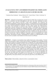
Silva, Santos and Silva49Percent fine(%)0.001 0.01 0.1 1 10 100Grain-size (mm)Fig. 2 Grain-size distribution curve for the bed material.Three locations within the main water stream wereselected for the soil samples, whose results are shown inFig. 2, and the Table 4 presents the grain-sizedistribution curves for each sample. The mean sedimentdiameter (d 50 ) varied between 0.45 and 0.71 mm.The available images for the study were obtained bysensor ETM, of Landsat 7 satellite, of the orbit 214 andPoint 65, year 2007. The color composites generatedfrom bands R1G4B3 were visually interpreted throughon screen digitizing. The image was georeferenced inGIS software, establishing a relationship between thecoordinates of the image and the acquired coordinates inthe field, in order to get a larger precision for the imageinterpretation. The image was transformed in UTMcoordinate system by the average of 1:25 000 scaledstandard topographic maps by using the first orderpolinomial and nearest neighbour resampling method.The supervised classification technique usingMaximum Likelihood was applied to classify theLandsat images of the microbasin. The aim of the imageclassification process is converting image data intothematic data. Fig. 3 presents the spectral interpretationand analysis of the geo-objects. Seven main types ofland use classes were identified within the basin:sugarcane, roads, grass, high capoeira, low capoeira,exposed soil, pineapple culture, and grass.Model simulationFor simulations, the WEPP watershed version was used.WEPP required climate, slope, management and soilinput files, which were assembled using the gatheredinformation. For the climate input file, breakpoint data(precipitation) and daily averages (temperature) wereused.Table 4. Soil samples to determine the grain-size distribution curvesGrain Sample 1 (%) Sample 2 (%) Sample 3 (%)-size(mm)coarser finer coarser finer coarser finer1.20 0.6 99.4 10.7 89.3 3.3 96.70.60 16.8 83.2 60.2 39.8 41.0 58.90.42 56.3 43.7 87.5 12.5 79.4 20.60.30 81.8 18.1 95.6 4.4 93.3 6.60.15 95.9 4.1 99.2 0.7 99.9 0.10.074 98.3 1.7 99.7 0.3 100.0 0.0Fig. 4 Discretization of Guaraira river experimental basinfor the WEPP model.Sub-division of hillslopes were carried out byoverlaying different thematic layers such as slopecoverage, soil coverage and land use coverage, so thateach hillslope is characterized by topography, soil, andland use. Parameters of the watershed such as overlandand channel slope, channel length and hillslope lengthwere extracted from different thematic layers (i.e.contour, slope and drainage map). The number ofchannels identified for each sub-watershed is presentedin Fig. 2 and Table 5Crop characteristics required for hydrologicalcalculation were taken from the WEPP crop databaseand supplemented with site-specific data. Soilerodibilities were calculated according to the WEPPrecommendation.Based on the field layout and topography, thewatershed area was divided into 22 sub-basins, whichwere connected through 10 channels. For each subbasin,a representative hillslope was selected and then, ifnecessary, it was divided into different overland flowelements according to the existing soil-vegetationcondition (Fig. 3).Table 5 presents the simulation results for each basinchannel element, and Table 6 shows the simulationresults for each basin plane element. The predicted soilloss values using WEPP model were reasonably good,based on the range of the observed values as publishedby Santos & Silva (2007) and Silva et al. (2007) to thesame basin.Journal of Urban and Environmental Engineering (JUEE), v.1, n.2, p.44-52, 2007

Silva, Santos and Silva50Table 5. Channel characteristicsChannelRunoff(m³/year × 10 5 )Sedimentyield(ton/year)ContributingchannelhillslopeC1 0.5 137 6 11, 12, 13C2 1.8 353 4 4, 5, 6C3 1.4 250 4 1, 2, 3C4 3.6 792 5 7, 8C5 4.4 1,314 6 9, 10C6 4.9 1,536 8 -C7 0.3 126 6 16, 17, 18C8 6.1 2,024 9 14, 15C9 6.6 2,297 10 19, 20C10 7.0 2,655 - 21, 22Fig. 3 Land use in Guaraíra River Experimental Basin.Further, the model parameters could be optimizedusing a genetic algorithm as presented by Duan et al.(1992), Sorooshian et al. (1993), and Santos et al.(2003).The obtained results showed the susceptible areas tothe erosion process within Guaraíra River Basin, andthat the mean sediment yield could be in the order of 21t/ha/year (in an area of 574 ha). The results also showedthat the computed soil losses was considered moderatebased on the four classes of basin soil loss as proposedby FAO (1967) in ton year/ha: (a) < 10 = very low; (b)10–50 = moderate; (c) 50–200 = high; and (d) 50–120= very high.The results demonstrate that reliable assessment ofthe available sediment yield models requires accuratesediment data collection which is most confidentlyobtained through development of sediment graphs.Moreover, preparation of input data for the modelrequirements may also lead to better and reliablejudgment.Table 6. Simulation results for each sub-basinHillslopesElement area Runoff volumesSoil lossesSediment yield(ha)(m³ year × 10 4 )(ton year)(ton year)H1 4.13 0.6 1.13 0.76H2 14.47 1.7 14.00 2.65H3 108.29 12.0 101.23 19.79H4 142.32 16.0 133.49 26.05H5 7.18 0.8 7.34 1.32H6 13.4 1.5 13.09 2.45H7 10.08 1.6 2.77 1.85H8 12.48 2.0 3.43 2.29H9 48.16 5.4 45.87 8.81H10 14.89 1.7 14.77 2.73H11 32.25 3.7 31.46 5.90H12 6.58 1.0 1.81 1.21H13 4.21 0.5 4.30 0.77H14 26.56 4.2 7.30 4.86H15 34.78 3.9 32.87 6.37H16 4.46 5.2 4.56 0.81H17 10.44 1.2 10.34 1.92H18 10.77 1.7 2.95 1.97H19 22.89 2.6 21.70 4.20H20 15.44 2.5 4.24 2.83H21 12.87 2.0 3.53 2.35H22 16.53 2.6 4.55 3.03Journal of Urban and Environmental Engineering (JUEE), v.1, n.2, p.44-52, 2007

Silva, Santos and Silva51Conclusion and recommendationsThe present research was conducted in the GuaraíraRiver Experimental Basin in Brazil, located innortheastern Brazil to assess the applicability of thewell-known WEPP model, remote sensing and GIStechniques for sediment yield prediction and the basinland use.The use of geoinformation techniques was verysuccessful in addressing the study objectives. Throughthese techniques, it was possible to identify and map theerosion areas and classify the land cover types withinthe studied area. Therefore, this study showed thatremote sensing and hydrologic modeling could be auseful tool for identification and analysis of soil lossand runoff in the Guaraíra river basin.The soil loss results, simulated by the WEPP model,showed that these losses within the basin could beconsidered moderate, around 21 ton/year ha, and thatthe planes H3 and H4 presented the largest losses(approximately 100 t/year ha).The presented simulation procedure are according tothe comments of Lakshmi (2004): the satellite remotesensing could be used to address to (a) advance theability of hydrologists worldwide to predict the fluxes ofwater and associated constituents from ungauged basins,along with estimates of the uncertainty of predictions;(b) predict the fluxes of water by using vegetation,surface air temperatures as inputs to hydrologicalmodels and surface temperature and soil moisture asvalidation variables in the intermediate step tocalculation of overland flow and stream flow; (c)advance the knowledge and understanding of climaticand landscape controls on hydrological processes toconstrain the uncertainty in hydrologic predictions,since the spatial mapping of land surface areas helps toidentify regions of saturation/high vegetation contentalong with surface flow characteristics, infiltrationdominated and/or runoff dominated; and (c) advance thescientific foundations of hydrology, and provide ascientific basis for sustainable river basin management.Future estimation of water resources requires anaccurate prediction of sources of surface and subsurfacewater, both of which can be mapped in space with theuse of satellite remote sensing. Tracking fresh waterestimates from space is a challenging problem that canbe solved by a combination of satellite sensors andexisting gauge networks (Lakshmi, 2004; Vrieling, 2006).Indeed, prediction of ungauged water resources isfast becoming a well-defined and important problem insatellite hydrology.Acknowledgment This research was financiallysupported by MCT/CT-Hidro/CNPq (n. 13/2005). Theauthors are also CNPq scholars.REFERENCESCavalcante, A. L. (2005). Bacia do Rio Guaraíra: propriedadeshidroclimatológicas e físicas do solo. Technical report in CivilEngineering Undergraduation course. João Pessoa, 47p.Chu, S.T. (1978). Infiltration during an unsteady rain. Water Resour.Res 14(3), 461−466.Cyr, L., Bonn, F. & Pesant, A. (1995). Vegetation indices derivedfrom remote sensing for an estimation of soil protection againstwater erosion. Ecol. Modelling 79(1-3), 277−285.Duan, Q., Sorooshian, S. & Gupta, V. (1992). Effective and efficientglobal optimization for conceptual rainfall-runoff models. WaterResour. Res 28(4), 1015−1031.Elliot, W.J., Liebenow, A.A., Laflen, J.M. & Kohl, K.D. (1989). Acompendium of soil erodibility data from WEPP cropland soilfield erodibility experiments. NSERL Report, vol. 3. AgriculturalRes. Service, National Soil Erosion Res. Lab., 316 p.F.A.O. - Food and Agriculture Organization (1967). La erosión delsuelo por el água. Algunas medidas para combatirla en las tierrasde cultivo. Cuadernos de Fomento Agropecuário daOrganización de Las Naciones Unidas 81, 207.Flanagan, D.C. & Nearing, M.A. (1995). USDA-Water ErosionPrediction project: Hillslope profile and watershed modeldocumentation. NSERL Report n. 10. USDA-ARS National SoilErosion Research Laboratory, West Lafayette, 47097−1196.Flanagan, D.C., Renschler, C.S. & Cochrane, T.A. (2000).Application of the WEPP model with digital geographicinformation. Proceedings of the 4th International Conference onIntegrating GIS and Environmental Modeling (GIS/EM4).Foster, G.R. & Meyer, L.D. (1972). A closed-form soil erosionequation for upland areas. In: Sedimentation (ed. by Shen, H.W.),Colorado State University, Fort Collins.Foster, G.R., Flanagan, D.C., Nearing, M.A., Lane, L.J., Risse, L.M..& Finkner, S.C. (1995). Hillslope erosion component. Flanagan,D. C. & Nearing, M. A. (eds.). USDA Water erosion predictionproject: hillslope profile and watershed model documentation.Report n. 10, USDA-ARS National Soil Erosion Research.Feoli, E., Vuerich, L.G. & Zerihun, W. (2002). Evaluation ofenvironmental degradation in northern Ethiopia using GIS tointegrate vegetation, geomorphological, erosion, and socioeconomicfactors. Agric., Ecosystems and Environ. 91(1-3),313−325.Huang, C.-H. & Bradford, J.M. (1993). Analysis of slope and runofffactors based on the WEPP erosion model. Soil Sci Soc Am J. 57,1176−1183.Jain, S.K. & Dolezal, F. (2000). Modeling soil erosion using EPICsupported by GIS, Bohemia, Czech Republic. J. Environ. Hydrol.8, 1−11.Jakubauskas, M.E., Whistler, J.L., Dillworth, M.E. & Martinko, E.A.(1992). Classifying remotely sensed data for use in an agriculturalnon-point source pollution model. J. Soil and Water Conser.47(2), 179−183.Jürgens, C. & Fander, M. (1993). Soil erosion assessment andsimulation by means of SGEOS and ancillary digital data. J.Remote Sens. 14(15), 2847−2855.Khan, M.A., Gupta, V.P. & Moharana, P.C. (2001). Watershedprioritization using remote sensing and geographical informationsystem: a case study from Guhiya, India. J. Arid Environs. 49(3),465−475.Lakshmi, V. (2004). Use of satellite remote sensing in hydrologicalpredictions in ungaged basins. Proceedings of the XXth ISPRSCongress. Istanbul, 2004.Mati, B.M., Morgan, R.P.C., Gichuki, F.N., Quinton, J.N., Brewer,T.R. & Liniger, H.P. (2000). Assessment of erosion hazard withthe USLE and GIS: a case study of the Upper Ewaso Ng’iro Northbasin of Kenya. J. of Applied Earth Observation andGeoinformation 2(2), 78−86.Journal of Urban and Environmental Engineering (JUEE), v.1, n.2, p.44-52, 2007

Silva, Santos and Silva52Millward, A.A. & Mersey, J.E. (1999). Adapting the RUSLE tomodel soil erosion potential in a mountainous tropical watershed.Catena, 38(2), 109−129.Nearing, M.A., Deer-Ascough, L. & Laflen, J.M. (1990). Sensitivityanalysis of the WEPP hillslope profile erosion model. Trans.ASAE 33(3), 839−849.Nearing, M.A., Liu, B.Y., Risse, L.M. & Zhang, X. (1995). Curvenumbers and Green-Ampt effective hydraulic conductivities.Water Resour. Bul. 32(1), 125−136.Pudasaini, M., Shrestha, S. & Riley, S. (2004). Application of WaterErosion Prediction Project (WEPP) to estimate soil erosion fromsingle storm rainfall events from construction sites. Proceedingsof the 3rd Australian New Zealand Soils Conference, 5-9December 2004, University of Sydney, Australia.Pullar, D. & Springer, D. (2000). Towards integrating GIS andcatchment models. Environ. Modelling & Software 15, 451−459.Rawls, W.J. & Brakensiek, D.L. (1983). A procedure to predictGreen and Ampt infiltration parameters. In: Proceedings of ASAEConference on Advances in Infiltration, Chicago, IL. ASAE, St.Joseph, 102−l 12.Risse, L.M., Nearing, M.A. & Savabi, R. (1992). An evaluation ofhydraulic conductivity prediction routines for WEPP using naturalrunoff plot data. Trans. ASAE, Paper 92−2142.Risse, L.M., Nearing, M.A. & Zhang, X.C. (1995). Variability inGreen-Ampt effective hydraulic conductivity under fallowconditions. J. Hydrol. 169, 1−24.Romero C.C., Stroosnijder L. & Baigorria G.A. (2007). Interrill andrill erodibility in the northern Andean Highlands, Catena 70(2),105−113.Saghafian, B., Van Lieshout, A.M. & Rajaei, H.M. (2000).Distributed catchment simulation using a raster GIS. Environ.Modelling and Software 2, 199−203.Santos, C.A.G. & Silva, R.M. (2007). Assessing erosion usingWEPP model with GIS for an experimental basin in northeasternBrazil. Proc. XXIV General Assembly IUGG, Perugia, Italy,IAHS, 2007.Santos, C.A.G., Srinivasan, V.S., Suzuki, K. & Watanabe, M. (2003)Application of an optimization technique to a physically basederosion model. Hydrol. Processes 47, 989–1003, doi:10.1002/hyp.1176.Shrimali, S.S., Aggarwal, S.P. & Samra, J.S. (2001). Prioritizingerosion-prone areas in hills using remote sensing and GIS: a casestudy of the Sukhna Lake catchment, Northern India. Environ.Modelling and Software 3, 54−60.Silva, R.M., Santos, C.A.G.; Silva, L.P., Silva, J.F.C.B.C. (2007).Soil loss prediction in Guaraíra river experimental basin, Paraíba,Brazil based on two erosion simulation models. Revista Ambi-Agua 2(3), 19−33.Sorooshian, S., Duan, Q. & Gupta, V.K. (1993). Calibration ofrainfall-runoff models: application of global optimisation to thesacramento soil moisture accounting model. Water Resour. Res.29(4), 1185−1194.SUDENE (1987). Levantamento exploratório-reconhecimento desolos do Estado da Paraíba. Recife, SUDENE, 350 p.Van der Sweep, R.A. (1992). Evaluation of the Water ErosionPrediction Project’s watershed version hydrologic component ona semi-arid rangeland watershed. Thesis, University of Arizona,Tucson.Vrieling. A. (2006). Satellite remote sensing for water erosionassessment: a review. Catena 65, 2−18.Wischmeier,W.H. & Smith, D.D. (1978). Predicting rainfall erosionlosses. Admin. U.S. Dept. Agr. Washington, D.C. AgricultureHandbook. Sci. and Educ., n. 357, 58 p.Journal of Urban and Environmental Engineering (JUEE), v.1, n.2, p.44-52, 2007

ISSN 1982-3932J U E EJournal of Urban and EnvironmentalEngineering, v.1, n.2 (2007) 53–60ISSN 1982-3932doi: 10.4090/juee.2007.v1n2.053060Journal of Urban andEnvironmental Engineeringwww.journal-uee.orgDESIGN AND DEVELOPMENT OF A 1/3 SCALE VERTICALAXIS WIND TURBINE FOR ELECTRICAL POWERGENERATIONAltab Hossain 1∗ , A.K.M.P. Iqbal 1 , Ataur Rahman 2 , M. Arifin 1 and M. Mazian 11 Department of Mechanical Engineering, Faculty of Engineering, Universiti Industri Selangor, Malaysia2 Department of Mechanical Engineering, International Islamic University Malaysia, MalaysiaReceived 13 May 2007; received in revised form 3 November 2007; accepted 5 November 2007Abstract:Keywords:This research describes the electrical power generation in Malaysia by the measurementof wind velocity acting on the wind turbine technology. The primary purpose of themeasurement over the 1/3 scaled prototype vertical axis wind turbine for the windvelocity is to predict the performance of full scaled H-type vertical axis wind turbine.The electrical power produced by the wind turbine is influenced by its two major part,wind power and belt power transmission system. The blade and the drag area systemare used to determine the powers of the wind that can be converted into electric poweras well as the belt power transmission system. In this study both wind power and beltpower transmission system has been considered. A set of blade and drag devices havebeen designed for the 1/3 scaled wind turbine at the Thermal Laboratory of Faculty ofEngineering, Universiti Industri Selangor (UNISEL). Test has been carried out on thewind turbine with the different wind velocities of 5.89 m/s, 6.08 m/s and 7.02 m/s.From the experiment, the wind power has been calculated as 132.19 W, 145.40 W and223.80 W. The maximum wind power is considered in the present study.Belt power transmission system; Reynolds number; wind power; wind turbine© 2007 Journal of Urban and Environmental Engineering (JUEE). All rights reserved.∗ Correspondence to: Altab Hossain, Tel.: +6-03 3280 5122 Ext 7187; Fax: +6-03 3289 7335.E-mail: altab75@unisel.edu.my

Hossain, Iqbal, Rahman, Arifin and Mazian55longer, and allow for better surge protection andgrounding. The United States Department of Energy hasrecently set up a schedule to implement the latestresearch in order to build wind turbines with a higherefficiency rating than is now possible (the efficiency ofan ideal wind turbine is 59.3 percent (Milligan & Artig,1999). That is, 59.3 percent of the wind’s energy can becaptured. Turbines in actual use are about 30 percentefficient). The United States Department of Energy hasalso contracted three corporations to investigate ways toreduce mechanical failure. This project began in thespring of 1992 and will extend to the end of the century.Wind turbines will become more prevalent in upcomingyears. The turn of the century should see wind turbinesthat are properly placed, efficient, durable, andnumerous. From the investigation of this wind turbinebackground, an H-type, vertical axis wind turbine hasbeen designed and built in thermal LaboratoryUniversiti Industri Selangor that has the capability toself-start. In addition, this turbine has been designed toallow a variety of modifications such as blade profileand pitching to be tested. The first part of the designprocess, which included research, brainstorming,engineering analysis, turbine design selection, andprototype testing have been incorporated. Using dataobtained through proper investigation results, the finalfull-scale turbine has been designed and built.Wind turbines can be separated into two types basedby the axis in which the turbine rotates namelyhorizontal axis wind turbine (HAWT) and the verticalaxis wind turbine (VAWT). HAWT has difficultyoperating in near ground, turbulent winds because theiryaw and blade bearing need smoother, more laminarwind flows, difficult to install needing very tall andexpensive cranes and skilled operators, downwindvariants suffer from fatigue and structural failure causedby the turbulence and height can be a safety hazard forlow-altitude aircraft. Other than that, the aerodynamicsof a horizontal-axis wind turbine is complex. The airflow at the blades is not the same as the airflow faraway from the turbine. The very nature of the way inwhich energy is extracted from the air also causes air tobe deflected by the turbine. In addition, theaerodynamics of a wind turbine at the rotor surfaceincludes effects that are rarely seen in otheraerodynamic fields. A wide variety of VAWTconfigurations have been proposed. The Darrieusvertical type wind turbine is the most common and usused extensively for power generation. However, theDarrieus turbine suffered from structural problems aswell as a poor energy market.To improve the performance of a wind turbine, thisstudy has been concentrated on design and built an 1/3scale H-type, vertical axis wind turbine that has thecapability to self-start due to the wind flow and efficientperformance of the VAWT that could lead to a changein the standard thinking of how wind energy isharnessed, and may spur future VAWT design andresearch. The study on the enhanced performance of thewind turbine is also given by incorporating dragdevices.WIND TURBINE DESIGNTheoretical analysisThe belt drive system consists of several parts of thebelt drive calculation and the V–Type belt is consideredin this study. Thus the main calculation that has beendone at this system are angle of wrap for small and largepulley, belt length, pulley speed, the tension ratio andthe power transmitted by the belt. The structure of theV-belt is shown in Fig. 1, which illustrates the mainparts in V-belt such as the large pulley diameterindicated by the number 3 and the small pulley by thenumber 2 and the angle of wrap of large pulleyindicated by θ 3 and small pulley by θ 2 . C indicates thecentered radius between large and small pulleys.2θ 2θ 33Fig. 1 The structure of the V-belt.Angle of wrap for large pulleyAngle of wrap for large pulley is defined as (Joseph etal., 2004)−1 3 2θ = °+ (1)3180 2sinD − D2CUsing large pulley diameter D 3 as 30.48 × 10 -2 m, smalldiameter D 2 as 5.08 × 10 -2 m and the radius C as 0.3048m in Eq. (1), the angle of wrap for the large pulley isobtained as θ 3 = 229.25°.Angle of wrap for small pulleyAngle of wrap for small pulley is defined as (Joseph etal., 2004)−1 3 2θ = °− (2)2180 2sinD − D2CUsing the same values as mentioned above in Eq. (2),angle of wrap for the small pulley is obtained as θ 2 =130.75°.CJournal of Urban and Environmental Engineering (JUEE), v.1, n.2, p.53-60, 2007

Hossain, Iqbal, Rahman, Arifin and Mazian56Centered radius lengthCentered radius length is defined as (Joseph et al.,2004)( D − D ) 2πL C ( D D )2 4C3 2= 2 +3+2+ (3)Using large pulley diameter D 3 of 30.48 × 10 -2 m,small pulley diameter D 2 as 5.08 × 10 -2 m and thecentered radius C as 0.3048 m in Eq. (3), the radiuslength is obtained as L =1.221 m.Tension ratio tide side over slack sideTension ratio of tide side over slack side is defined as(Joseph et al., 2004):TT( )⎡µθ⎤13= ln ⎢ ⎥22.3⎣⎦(4)Using tension at tide side T 1 as 166.77N, tension atslack side T 2 as 107.94N and pulley velocity V as 2.84m/s in Eq. (7), power transmitted by the belt is obtainedas P B = 167.08 W.Prototype designThe components of the 1/3 scaled vertical axis windturbine are designed by using the CATIA software inthe Structural Laboratory in Unisel and assembledtogether to predict the full scale. The wind turbine is athree bladed with tapered wing sections connected to therotor of the generator and has been tested at an openhall. The corner sharp has been used as aerofoil for thewind turbine blade by producing a controllableaerodynamic force with its motion through the windflow as shown in Fig. 2. The other main componentsthat have been designed and used to construct the windturbine are described in the following sections.where, the coefficient of belt friction µ is 0.25, θ 3 is theaforementioned angle of wrap of small pulley in radians(4 rad), T 1 is tension at tide side and T 2 is tension atslack side.Using the values as mentioned above in Eq. (4),tension ratio of tide side over slack side is obtained asT 1 /T 2 = 1.545.Tide side belt tensionTension of tide side is defined as (Sorge, 1996)T 1 = Wg (5)By choosing the total weight W of the upper part ofturbine as 17 kg and adopting gravitational accelerationg as 9.81 m/s 2 in Eq. (5), tension of tide side is obtainedas T 1 = 166.77 N.Fig. 2 The shape of Aerofoil with 139.7 mm chord.Base and Base TableThe base material has been chosen as steel since itstands 6096 mm high and weighs 15 kg, and on its ownthe base does not support the torque and momentsproduced from the wind turbine, so a base extension anda connecting bracket have been designed. To connectthe 4 sheets of steel bracket to the steel base a bottombracket made of 38.10 mm × 762 mm steel has beenused. The 38.10 mm × 38.10 mm structure providesquick assembly and disassembly of the turbine basestructure.Slack side belt tensionUsing the value of T 1 in Eq. (4), tension of slack side isobtained as T 2 = 107.94 N.Pulley velocityVelocity of pulley is defined as (Joseph et al., 2004)3V πDN= (6)60Power transmitted by the beltThe power transmitted by the belt is defined as (Josephet al., 2004)P B = (T 1 – T 2 )V (7)Fig. 3 Base table.The bottom bracket requires four simple cornerwelds and flat head bolts welded in position thatencourage quick assembly. Four sheets of 1219.20 mmJournal of Urban and Environmental Engineering (JUEE), v.1, n.2, p.53-60, 2007

Hossain, Iqbal, Rahman, Arifin and Mazian57× 2438.40 mm × 19.05 mm have been used to constructa base extension that gives a larger footprint on whichweights are placed. The main sheet is oriented with twosheets side-by-side, with two other sheets on top at 90degrees rotation to the bottom two sheets. This creates abase table of 2438.40 mm × 2438.40 mm dimensions asshown in Fig. 3.on the device, which has operated successfully. Beforestarting the operation, the battery terminal and alternatorterminal are checked properly and it is connected withthe lamp and switch. Then the wind turbine is allowedto rotate. Due to the rotation of the wind turbine bladevoltage is produced and the connected lamps are turnedon (Fig. 5).Shaft and BearingsThe shaft used in this design is the type of polishaft andits weight is 14 kg, being made from steel. The diameterof the shaft is 30 mm and its length is 2133.6 mm. Itssurfaces are very soft and make the shaft rotation verysmooth when attached to the bearing. Minimizing therequired start-up torque is essential for the wind turbineto self-start and thus, the success of the project. Thebearings that are used in the wind turbine design are notsalvageable.Bearings are very expensive, and for the particularsetup two roller bearings have been used that areprimarily centralized with the shaft. This combinationprovides the least amount of friction, while maximizingbearing life and maintaining safe operating conditions.The diameters of the bearings are 88 mm and weights300 g each.Support Arm and Drag DeviceSteel is used for the three support radial arms tomaintain a lightweight assembly with minimal inertial,moment, and centrifugal forces. The connecting armsprovide a means to mount the blades to the center shaft.A drag device has been made from a lightweight plastic(casting plastic) and mounted to the main shaft. Thelength of the drag device is about 762 mm and width is182.88 mm.Fig. 4 Final assembly of the prototype wind turbine.Wind Turbine Blade DesignThe top and bottom of each blade is a 1066.8 mm ×139.7 mm × 50.8 mm deep rectangular section to allowfor easier connections to the radial arms and passivepitching system. In this study the corner sharp has beenselected as the shape of the blade for its very highcapability to face the resistance of wind flow and fasterrotation during the wind flow.The final assembly of the wind turbine has been setat Thermal Laboratory in Universiti Industri Selangorand is shown in Fig. 4. There are 18 parts and 15 screwscombined together in the assembly process. The shaft isconnected to the main parts and to the alternator duringthe full assembly of this vertical axis wind turbine.Experimental ProcedureThe prototype of the Unisel wind turbine is installed atthe Thermal Laboratory in Universiti Industri Selangorand a number of preliminary tests have been carried outFig. 5 Experiment of power generation with wind turbine.Journal of Urban and Environmental Engineering (JUEE), v.1, n.2, p.53-60, 2007

Hossain, Iqbal, Rahman, Arifin and Mazian58Table 1. Free stream velocity and Reynolds numberSerial NumberFree streamvelocity (m/s)Reynolds number1 5.89 0.49 × 10 52 6.08 0.51 × 10 53 7.02 0.58 × 10 5The produced voltage readings and the respectiveturbine rotations are recorded. The ambient pressure andtemperature are recorded using the manometer andthermometer for the evaluation of air density in theLaboratory environment of Universiti Industri Selangor.The power produced by the wind speed is alsocalculated which is shown in the specimen calculationsection. The main test is performed at open hall in theThermal Laboratory of Faculty of Engineering,UNISEL, where wind speeds are measured between 4and 6 m/s, with gusts up to 7 m/s.During the test, the turbine has been run based on thedesign, then the blades are opened and the wind hasbeen propelled, and finally it has been checked aboutsufficient production of lift when the blades are closed.It has been seemed as though the turbine would slowdown too much in the regions where lift is not producedthus the blades are kept opening up just to allowrotation. Next the blades have been opened to check themaximum attainable rotational speed in the dragposition. In this position it is observed that there isplenty of windswept area to rotate the turbine.Specimen calculationAbsolute pressure p = 1.01 × 10 5 N/m 2 and temperature,T = 38.5 o C = 311.5K. Using equations of state forperfect gas the air density, ρ ∞ is 1.13 kg/m 3 and isdefined as (Bertin, 2002):pρ∞=(8)RTwhere, pressure p is 1.01 × 10 5 N/m 2 , temperature T is311.5 K, and gas constant of air R is 287.05 Nm/kg K.The air viscosity, µ ∞ is determined using theSutherland’s equation (Bertin, 2002) described below1⋅5−6Tµ∞= 1.458×10(9)T + 110.4where µ ∞ is the dynamic viscosity.At T of 311.5 K, Eq. (9) gives value of µ ∞ of 1.90 ×10 -5 kg/m s. Reynolds number based on the chord lengthis defined as (Anderson, 1996).ρ vc= (10)µ∞ ∞Re∞Using air density ρ ∞ of 1.13 kg/m 3 , free streamvelocity ν ∞ of 5.89 m/s; dynamic viscosity µ ∞ of 1.90 ×10 -5 kg/m s and chord length c of 0.1397 m in Eq. (10),Reynolds number is obtained as Re = 0.49 × 10 5 .For the remaining velocities the correspondingReynolds numbers are given in Table 1. For arectangular blade, frontal surface area for a singlesurface is defined as (Bertin, 2002):S = bc (11)For a wind turbine, total frontal surface area S T is1.145 m 2 and is defined as (Bertin, 2002):S T = (S 1 ) T + (S 2 ) T (12)where, the total frontal area for blade (S 1 ) T is 0.4482 m 2and the total frontal area for drag surface (S 2 ) T is 0.6968m 2 .Wind power of the turbine is defined as (Bench &Cloud, 2004)Pwind13= ρ∞STv(13)∞2where, the density of air ρ ∞ is 1.130kg/m 3 , the totalfrontal area S T is 1.145m 2 , and wind velocity ν ∞ is 5.89m/s.Putting the values into Eq. (13), we have:P31 ⎡kg ⎛m⎞⎤= × 1.130× 1.145× 5.89 × m × ⎜ ⎟ ⎥2 ⎢⎣m ⎝ s ⎠ ⎥⎦P wind = 132.19 W3 2wind ⎢ 3For the remaining velocities corresponding windpower are given in Table 2.RESULTS AND DISCUSSIONSExperiments have been carried out at open hall UNISELat the three different velocities of 5.89 m/s, 6.08m/s and7.02 m/s. Based on the measurement of velocity thewind power for this prototype is calculated at theprevious section and is given in Table 2. The calculatedvalues for the Reynolds number in Table 1 have beenpresented in the previous section.The further understanding of the relationshipbetween the variables measured as velocity as well ascalculated wind power and Reynolds number from thetest conducted has been discussed in term of graphs.Table 2. Velocities and Corresponding wind powerSerial No. Velocities (m/s) Wind power (W)1 5.89 132.192 6.08 145.403 7.02 223.80Journal of Urban and Environmental Engineering (JUEE), v.1, n.2, p.53-60, 2007

Hossain, Iqbal, Rahman, Arifin and Mazian59Reynolds numberThe higher values in Reynolds number indicate the windturbine has ability to produce more power due toincrease in value of the wind velocity and this value iscalculated and recorded in tests conducted at the windvelocity of 7.02 m/s.The Aerofoil geometrySelecting appropriate aerofoil to a 3-bladed vertical axiswind turbine is one of the most important designdecisions. Different profiles provide various advantagesand disadvantages that must be considered. However,the affection of this wind flow due to airfoils or bladesis very small and the amount of the force that dependson the blade during the rotation has been ignored. Inaddition, the blade that has been designed and used inthis model is not considered as NACA 0012 or NACA0015 which are preferable in the low Reynolds numberrange, but the shapes selected in the current project stillresponded and acted with a very high durability andefficient functional to the shaft to rotate during the windflow.The Drag Devices geometryThe drag devices that have been used in current projectprovide external support to the blade by collecting themaximum amount of wind flow and initializing therotation of the blade and the shafts. The drag devices arevery sensitive to small amounts of the wind flow and italways causes the blades and shaft to rotate even thewind velocity is very small in magnitude at theconsidered location. During the test conducted on thismodel the wind has been blocked by one of the opendrag, and diverted around the other. This is factorizingthe net torque which drives the open drag around theshaft and induces rotation of the turbine, which leads tocentrifugal forces. The rotational speed is increaseduntil a critical point at which the turbine is moving fastenough to be driven by the lift forces. Theopening/closing of drag mechanism is designed suchthat the centrifugal forces overcome the inertial forcesand direct forces at this critical speed. In particular, thedevice has a very strong torque characteristic at low tipspeed ratio, which means it is a self-starting. However,difficulties with commissioning of the torquemeasurement and control systems have delayed theacquisition of definite test data to date.Turbine feasibility comparisonsThe calculated wind power from the current 1/3 scalewind turbine and the overall comparisons of the existingturbine according to the type of connection used and theestimated costs are shown in Table 3.The University of Wollongong project has producedthe maximum wind power which of 700 W using aTable 3. Feasibility comparison of different wind turbineUniversity Type of Wind Power CostResearch connection velocity (m/s) (W) (US$)Wollongong Gearing System 25 700 820Griffith Gearing System 20 550 673UNISEL Belt & Pulley 6 167 253gearing system and Griffith University has producedelectrical power of 550 W using a similar system(Cooper & Kennedy, 2003; Kirke, 2003). The testedprototype in current project has been produced 167 Wusing the belt and pulley system. According to theevaluation of wind velocities, the current model canexceed the existing models if the wind velocity isincreased. The current prototype would be capable toproduce 567.33 W when the wind velocity increases to20 m/s and 709.17 W when the wind velocity increasesto 25 m/s. This overall comparison presents evidencethat the current prototype, which uses the pulley andbelt systems, is more feasible than the other models thatuses the gearing system in terms of cost and to producepower.ConclusionThe conclusions drawn from this investigation are asfollows:(a) Wind power produced by the prototype increasesmaximum of 1000 W with the increase ofmaximum wind velocity of about 12 m/s.(b) From the investigation there is evidence that thecurrent prototype is capable to produce 567.33 Wwhen the wind velocity increases to 20 m/s and 709W when the wind velocity increases to 25 m/s.NomenclatureSymbol Meaning Unitp Absolute pressure (N/m²)T Temperature (K)R Gas constant (Nm/kg K)ρ ∞ Air density (kg/m³)µ ∞ Air viscosity (kg m/s)ν ∞ Free stream velocity (m/s)c Chord length (m)R e Reynolds number (Dimensionless)B Blade height (m)S 1 Blade frontal surface area (m²)S 2 Drag device frontal area (m²)S T Total frontal area (m²)P wind Wind power (W)Journal of Urban and Environmental Engineering (JUEE), v.1, n.2, p.53-60, 2007

Hossain, Iqbal, Rahman, Arifin and Mazian60Acknowledgment The authors are grateful for thesupport provided by financial assistance from theUniversiti Industri Selangor, and faculty of Engineeringfor the overall facilities.REFERENCESAnderson, J.D.Jr. (1999) Aircraft Performance and Design. McGrawHill Companies Inc., U.S.A.Bench, S.E., Cloud, P.K. (2004) The Measure, Predict and Calculatethe Power response of an Operating Wind Turbine. 1 st Ed.,London, Jepson Pub, 366 p.Bertin, J. J. (2002) Aerodynamics for the Engineer. New Jersey,Prentice Hall, Inc., U.S.A.Cooper, P., Kennedy, O. (2003) Development and Analysis of aNovel Vertical Axis Wind Turbine. Bachelor. Thesis, Universityof Wollongong, NSW 2522, Australia.Fitzwater, L.M., Cornell, C.A., Veers, P.S. (1996) UsingEnvironmental Contours to Predict Extreme Events on WindTurbines. Wind Energy Symp., AIAA/ASME, 9, 244–258.Hammons, T.J. (2004) Technology and Status of Developments inHarnessing the World’s Untapped Wind-Power Resources.Electricity Power Components and Systems. No.12, p. 32.Joseph, E.S, Charles, R.M, Richard, G.B. (2004) MechanicalEngineering Design. 7 th Ed., United State of America. p. 1030.Keith, David W. (2005) The Influence of Large-Scale Wind Poweron Global Climate. Proc. National Academy of Sciences,Washington D.C, Vol. 101, pp. 12–56.Kirke, B.K. (2003) Evaluation of self-starting vertical axis windturbines for stand alone applications. PhD Thesis, GriffithUniversity, Australia.Milligan, M.R. & Artig, R. (1999) Choosing Wind Power PlantLocations and Sizes Based on Electric Reliability Measures UsingMultiple-Year Wind Speed Measurements. National RenewableEnergy Laboratory, 8, 52p.Monett, G., Poloni, C. & Diviacco, B. (1994) Optimization of windturbine positioning in wind farms by means of large development.J. of Wind Engng and Ind. Aerod 23(4), 105–16Sorge, F. (1996) A qualitative-quantitative approach to v-beltmechanics. ASME, J. of Mechanical Design 118(8).Journal of Urban and Environmental Engineering (JUEE), v.1, n.2, p.53-60, 2007

ISSN 1982-3932J U E EJournal of Urban and EnvironmentalEngineering, v.1, n.2 (2007) 61–69ISSN 1982-3932doi: 10.4090/juee.2007.v1n2.061069Journal of Urban andEnvironmental Engineeringwww.journal-uee.orgSTUDY OF SENSITIVITY OF THE PARAMETERS OF AGENETIC ALGORITHM FOR DESIGN OF WATERDISTRIBUTION NETWORKSPedro L. Iglesias ∗ , Daniel Mora, F. Javier Martinez and Vicente S. FuertesMultidisciplinar Center of Fluids Modeling (CMMF), Polytechnical University of Valencia, SpainReceived 11 May 2007; received in revised form 15 June 2007; accepted 19 August 2007Abstract:Keywords:The Genetic Algorithms (GAs) are a technique of optimization used for waterdistribution networks design. This work has been made with a modified pseudo geneticalgorithm (PGA), whose main variation with a classical GA is a change in thecodification of the chromosomes, which is made of numerical form instead of thebinary codification. This variation entails a series of special characteristics in thecodification and in the definition of the operations of mutation and crossover. Initially,the work displays the results of the PGA on a water network studied in the literature.The results show the kindness of the method. Also is made a statistical analysis of theobtained solutions. This analysis allows verifying the values of mutation and crossingprobability more suitable for the proposed method. Finally, in the study of the analyzedwater supply networks the concept of reliability in introduced. This concept is essentialto understand the validity of the obtained results. The second part, starting with valuesoptimized for the probability of crossing and mutation, the influence of the populationsize is analyzed in the final solutions on the network of Hanoi, widely studied in thebibliography. The aim is to find the most suitable configuration of the problem, so thatgood solutions are obtained in the less time.Algorithms; design; water networks; reliability© 2007 Journal of Urban and Environmental Engineering (JUEE). All rights reserved.∗ Correspondence to: Pedro L. Iglesias Rey, Tel.: +34 96 3 879890; Fax: +34 96 3879781.E-mail: mpiglesia@gmmf.upv.es

Rey, Meliá, Martinez and Fuertes62INTRODUCTIONThe design of water distribution networks is extremelycomplex. It is well-known that when the diameters ofthe conductions are chosen as decision variables, therestrictions are implied functions of these variables ofdecision, so the space’s region of solutions is a noconvex type and the objective function becomesmultimodal. Traditionally, water distribution networkdesign, upgrade, or rehabilitation has been based onengineering judgment.However, in the last three decades a significantamount of research has focused on the optimal design ofwater distribution networks. Initially, researchers haveused linear programming to optimize a design of a pipenetwork (Alperovits & Shamir, 1977). Later studiesapplied nonlinear programming to the network designproblems. Some examples are Su et al. (1987) that usednon linear programming to optimize looped pipenetworks or Lansey & Mays (1989), whose model wasable to simulate pumps, tanks and multiple loadingcases.The application of heuristic techniques ofoptimization allows the search beyond these localminimums, which generally ample the field search andwith it the capacity to obtain better solutions. Theevolutionary algorithms are methods of search ofsolutions that are based in the natural beginning of theevolution. Inside the evolutionary algorithms, we canfind Genetic Algorithms (GA), Particle Swarm Optimization(PSO), Ant Colony, Harmony Search, and so on.Some investigators have compared these techniquesto each other (Zecchin et al., 2007), but it is difficult tosay that one of them is clearly better than the others.Genetics algorithms (GAs) are a searching methodbased on Darwin´s evolution theory (Holland, 1992). Itworks identically to the evolution of a population that isput under similar random actions to which they act inthe biological evolution (mutations and geneticrecombination). The individuals best adapted surviveand the less ones are discarded, based in someestablished criteria.Most of these methods, for a given network layoutand demand, consider the minimization cost of a pipenetwork as the objective. In the field of hydraulicengineering, previous works like those of Goldberg(1987), Savic & Walters (1997), Iglesias et al. (2006),Fujiwara & Khang (1990) or Cunha & Sousa (1999),reflects the importance that these algorithms areimplementing in the optimal design of water distributionnetworks.Branched water distribution networks will havesevere consequences in terms of reliability under failureconditions. To improve the performance of a waterdistribution network under failure conditions, Goulter &Bouchart (1990) have solved a reliability constrainedleast cost optimization problem.Loops in a network increase its reliability, so that thesystem will have sufficient capacity to deliver duringmechanical or hydraulic failures. Mora et al. (2006)uses GA for compare design of water distributionsystems with and without reliability in the network.However, explicit consideration of reliability in anoptimization model is difficult, and there are nouniversally accepted definitions for reliability.In the same way, GAs have been used for waternetwork rehabilitation (Halhal et al., 1997) and for thecalibration of water distribution models (Balla &Lingireddy, 2000), where the manual adjustment ofuncertain parameters as the pipe roughness coefficientsand the water demand at nodes is highly inefficient andoften unsuccessful.This work shows the development of a method forthe optimal design of water distribution networks basedon the GA use. The aim is to minimize the necessarycosts of investment for the implantation of a certainsystem, starting from the topological layout and thedemands and requirements of pressure in the nodes. Theproposed method develops a code based on the use ofnumerical chromosomes instead of binarychromosomes. It is also introduced the optimization ofthe different parameters which influence in theminimum achievement, like the probabilities ofmutation and crossover, and the population size whichthe algorithm will work with.METHODOLOGYThe GAs are systematic methods for the resolution ofsearching and optimization problems that apply thesame methods of the biological evolution, as theselection based on the population, reproduction andmutation.Traditionally, the GAs have been methods adaptedfor problems formulated in binary variables but notadvisable for other searching methods. However, in thepresent work a formulation of the problem is introducedbased on a numerical codification, non binary, of thesolution.The random character of the method does notguarantee a complete exploration of the space ofsolutions, nor supposes guarantee to reach a minimumof the objective function. However, the method offers aset of good solutions that try to improve. The work’selements of a GAs are defined perfectly in Iglesias et al.(2002) and in Matías (2003). Hereby is proposed a briefdescription emphasizing the adaptations made for thepseudo-genetic algorithm (PGA).The gene is the basic unit of information that adoptsa binary value (0/1). In the method each one of thedecision variables can have a rank of possible differentsolutions, which is represented with an alphanumericalvariable. With this codification is possible to identifyeach gene with a variable decision, which did notJournal of Urban and Environmental Engineering (JUEE), v.1, n.2, p.61-69, 2007

Rey, Meliá, Martinez and Fuertes63Fig. 1 Definition of chromosome and gene in a genetic algorithm(GA) and of the proposed pseudo-genetic algorithm (PGA).happen in the classic GA. In the design of waterdistribution networks, each gene is represented with anumber or a letter that identifies the diameter of eachone of the lines (Fig. 1). The detail on the codificationand the variables can follow in Iglesias et al. (2002).A chromosome represents a solution to the problem.This solution is constituted by a serial of genes thatdefines a unique solution of the optimization process.When designing a water distribution network withoutconsidering pumps and valves, the genes are therepresentation of the diameter that adopts each tube ineach one of the solutions.In order to solve the optimization problem it isnecessary to have a discrete set of possible solutions(chromosomes). This set of chromosomes is what alsoforms the population of the GA and the PGA. In thePGA a generic chain X is constituted by an equalnumber of genes to the number of decision variables(NVD), so that generic chain i of a P population isdefined as a vector of numerical values.{ 1 2 }i i i iX X X X N= , ,…, (1)VDThe characteristic that measures “kindness” orcapacity of a certain chromosome’s survival regardingthe others is known like aptitude. The aptitude of acertain generic chromosome is identified through thevalue that adopts the objective function for the codifiedsolution. In the case of the PGA proposed for designand extension of supplying networks this objectivefunction is defined asN N NVD S Ri∑ j( j) j ∑∑ k. s ( min, k k,s)(2)iFX ( ) = C X ⋅ L+ λ⋅ δ ⋅ H −Hj= 1 s= 1 k=1where C j is the associated unit cost to the decisionvariable’s value contained in link j of chromosome i;and L j is the length of conduction of pipe j. Moreover,they are N R imposed restrictions that must achieve thepossible solutions of the problem. These restrictionshave been including through a penalty in the total costof the solution that later affects the aptitude of thechromosome.The restrictions that must be fulfilled are thederived ones to satisfy the restrictions with minimumpressure height (H min,k ) in each node k. Theserestrictions must be verified in all the analyzed scenesN S , that usually are the on-speed operation of the systemand its operation under the scene of failure of some ofthe conductions. The function penalty represents thedifference between the head height of the node k inscene s (H k,s ) and the required minimum height (H min,k ).In order to compute this penalty two variables aredefined. One of them (δ k,s ) is a binary variable thatadopts value 1 if H k,s < H min,k , and it adopts null value inopposite case. The parameter λ represents a weightfunction that establishes the penalty’s value for notverifying the restrictions of minimum pressure in thenodes. Pressure is considered as a hard constraint, and λis big enough (10 7 ) for reject all solutions that violatesthe constraint.In this paper the only network components that areconsidered are the pipes, but it is possible incorporateelements as pumps, tanks, valves and reservoirs withoutinvalidating the algorithms.The method of the proposed PGA tries the evolutionof a random population through a parallelism similar tothe laws of the natural selection, as it happens with theclassic GA (Matías, 2003; Iglesias et al., 2002). This isobtained through three basic processes: reproduction,crossover and mutation.The reproduction is the process through we selectbetween the chromosomes of the P population, thosethat will survive the following generation. Between allthe existing methods of reproduction (Matías, 2003) it isbeen selected the constant reproduction method.This method orders the individuals of a population inincreasing order according to its cost: from the cheapestindividual to the most expensive. Later, a probability isassigned to each chromosome of the population tobecome one of the following generation. Thisprobability will be included between a maximumprobability p max , associated with the individual ofsmaller cost, and a minimum probability, associated tothe solution of greater cost. Both probabilities aredefined aspβmax= pminNC2 − β= (3)Nwhen β is a constant whose value must be comprisedbetween 1.5 and 2 (Wang, 1991) and N C is the numberof chromosomes.The crossover process (Fig. 2) consists in matchingin a random way the chromosomes of the intermediatepopulation and making a change of the different genesfrom a certain crossover gene, determined in a randomway. It does not matter if two descendants of sameparents are matched, since it guarantees the perpetuationof an individual with good score. However, it is notadvisable to repeat this situation too much, since thepopulation could get dominated by the descendants ofsome gene, which could cause the falling of thecalculation in a local minimum.CJournal of Urban and Environmental Engineering (JUEE), v.1, n.2, p.61-69, 2007

Rey, Meliá, Martinez and Fuertes64Fig. 3 Process of mutation of a PGA.Fig. 2 Process of crossover.One of the fundamental characteristics of the PGA isthe effect generated when crossing differentchromosomes. If the codification is binary, thecrossover process cut the chain in a random point. Thiscan originate the fraction of the binary code thatidentifies one of the possible variables of decision. Incase of implementing the PGA the selection of acrossing link does not generate this effect. This is thereason using the PGA generates minor changepossibility in the final solutions that the classic GA.The mutation process is applied to the obtainedpopulation after the crossing and reproduction process.Once established the mutation frequency, for example,one by thousands, is examined each gene of eachchromosome when an individual is created from itsparents. If a random generated number is under thatprobability, the gene will change. If no, it will be left as it is.Once chosen the mutation gene this bit is determinedrandomly whether it must be increased or decreased inone unit. Fig. 3 shows the mutation process, where geneB could evolve to A or C. This is the way to determinethe value of the link in the following generation. Boththe crossing process and the chromosome’s codificationcause the generation of new alternatives in PGA beinginferior to the one of a classic GA. For this reason theprobability of mutation in the PGA is slightly superior.The mutation is a parameter which is not convenientto abuse; it is a generating mechanism of diversity, butalso it reduces the genetic algorithm to a random search.It is always more advisable to use other mechanisms ofdiversity generation, like increasing the size of thepopulation, or guarantee the randomness of the initialpopulation.This way, the size of the population will have to beenough in order to guarantee the diversity of solutions,and, in addition, it must grow with the number ofchromosome’s bits. The main problem that is generatedwhen using high populations is that convergence time ofthe algorithm is bigger. Therefore it is necessary toreach a commitment solution depending on theapproach of the problem.The following sections analyze the capacity of theproposed PGA to obtain equal or better solutions to theexisting ones in the references. It has been analyzeddifferent water distribution networks, determining theminimum cost of design them. The initials studies of theproposed model had been realized about Alperovits &Shamir network (1977), achieving the same minimumresults obtained in bibliography (Iglesias et al., 2006).However, the reduced size of this network did notallowed to deepen in the kindness of the method.Thus, working on the network of Hanoi, theinfluence of the different parameters has been analyzedon the final solution, dividing the work in two phases:First stage where the best combination of the crossoverand mutation probabilities are analyzed, and one secondphase, where from the first optimization the populationsize’s influence in obtaining the minimum value ofdesign is analyzed.In each calculation it is necessary to determinepressure in nodes and flow in lines. These calculationsare made by means of the model EPANET, developedby the Water Supply and Water Resources Division ofthe U.S. Environmental Protection Agency's NationalRisk Management Research Laboratory, whosefoundations can be followed in Iglesias (2004). Themassive treatment of simulations to obtain theparameters of the PGA has been made with a specificapplication, as it is described in Iglesias (2006).APPLICATION EXAMPLEThe analysis of the proposed model has been made onthe network of Hanoi (Fig. 4), as propose by Fujiwara &Khang (1990). As it is a water network of important sizeand with a real layout, there is a wide range of solutionsobtained with different models of design in thebibliography, which has allowed us to compare theresults of the different models of design.The network consists of one reservoir (node 1), 31demand nodes and 34 pipes. The minimum pressurehead required at each node is 30 m.One of the characteristics that contribute to definethe optimal solution of the network is the range ofdiameters used. For the study we used the original rangeof the bibliography (Table 1).The work displayed by Iglesias et al. (2006) showsthe results obtained by the different researchers, as wellas the obtained by the proposed method. This workdeals with fixed populations of 100 individuals, beingthe aim the optimization of crossover and mutationJournal of Urban and Environmental Engineering (JUEE), v.1, n.2, p.61-69, 2007

Rey, Meliá, Martinez and Fuertes65121110,00%100,00%323133 34 26 27 28252430 29 23211617181514131920 3 4 52109876Probability9,00%8,00%7,00%6,00%5,00%4,00%3,00%2,00%1,00%0,00%6.0816.1116.1426.1726.2026.2326.2636.2936.3236.3536.3836.4146.4446.4746.5046.5356.5656.5956.6256.6566.6866.7166.7466.7766.8076.8376.8676.8976.9286.9586.9887.018Thousands (u.m)Frequency of solutionsAccumulated probabilityFig. 5 Diagram of frequencies and accumulated probability of theobtained solutions.90,00%80,00%70,00%60,00%50,00%40,00%30,00%20,00%10,00%0,00%22Fig. 4 Network of Hanoi.parameters. Table 2 shows the solution’s variationobtained by some researchers, as well as itscorresponding total cost.It is worth mentioning that in the column Sol 2 ofTable 2 we consider the burst of the pipes that closeloop network. For this reason prevails as condition thatthe pressure restrictions must even verify when abreakdown takes place in any of the pipes and thisincreases the cost of the network.If we rely on the obtained minimum value, weobserve that the PGA improves those of all hiscompetitors but the one of Cunha & Sousa, in terms ofthe used heuristic method does not fulfil the pressurespecifications.In the solution where the reliability concept isintroduced, the cost of the network grows, logicalcircumstance, since the diameters to guarantee theprovision in case of breakage must be greater. In thereal case that one appears next has considered this fact,reason why all the given data already consider thereliability concept.ANALYSIS OF THE RESULTSOne of the main characteristics of a GA is that it worksin a random way. The characteristics of the method doTable 1. Range of diameters used for the design of the waterdistribution networkOriginal rangeNo. Diameter Diameter (mm) Cost (mu/m)A 304.8 45.73B 406.4 70.40C 508.0 98.39D 609.6 129.33E 762.0 180.75F 1016.0 278.281not guarantee with certainty the obtaining of the optimalvalue of the system. In addition, the obtained result cansuffer sometimes certain variations. In order to analyzethis randomness it is necessary to make statisticalanalyses that will study the influence that have thedifferent parameters from the PGA proposed in thesolution of the analyzed network, with the purpose ofoptimizing them to increase the probability of obtainingthe minimum.In a first study, the mutation and crossoverprobabilities were modified, maintaining the size of thechain constant. Later, from the best values obtained forboth parameters another study was made, with theobjective to study the influence of the population in thesearch of the best solution. For it they have been mademore than 50 000 simulations altogether. For thecalculation of these simulations we use a computersystem in parallel with 23 computers AMD Duron to1400 MHz and 128 MB of ram.Influence of crossover and mutation probabilityInitially a histogram is made (Fig. 5). This graphincorporates the accumulated probability of the obtainedsolutions. The graph allows to detect the more frequentsolutions, as well as to determine the probability ofobtaining a given solution better to one given. It isimportant to consider that the histogram represents thetotality of obtained costs, varying crossover andmutation probabilities, with a fixed population of 100individuals.In order to determine the influence of mutation andcrossover probability in the obtaining of the minimumcost value, we adopted the solution corresponding to6081 thousands of monetary units. This minimum wasconsidered the optimal value of design, as it was theminimum obtained. Fixed this value it has beenanalyzed for each value’s combination of mutation andcrossover, the probability that method PGA obtains theoptimal value. The representation of this rate of successobtaining the minimum is shown in Fig. 6. In it weremark that there are combinations of values of theJournal of Urban and Environmental Engineering (JUEE), v.1, n.2, p.61-69, 2007

Rey, Meliá, Martinez and Fuertes66Table 2. Comparison of diameters (mm) obtained as solution for the network of HanoiLineBibliography SolutionsObtained SolutionsMatías (1) Savic1 (2) Savic2 (3) Cunha (4) Sol 1 (5) Sol 2 (6)1 1016 1016 1016 1016 1016 12702 1016 1016 1016 1016 1016 12703 1016 1016 1016 1016 1016 10164 1016 1016 1016 1016 1016 10165 1016 1016 1016 1016 1016 10166 1016 1016 1016 1016 1016 7627 1016 1016 1016 1016 1016 7628 1016 1016 1016 1016 1016 7629 1016 762 1016 1016 1016 76210 762 762 762 762 762 609.611 609.6 762 609.6 609.6 609.6 609.612 609.6 609.6 609.6 609.6 609.6 50813 508 406.4 508 508 508 101614 406.4 406.4 406.4 406.4 406.4 76215 304.8 304.8 304.8 304.8 304.8 101616 304.8 406.4 304.8 304.8 304.8 101617 406.4 508 406.4 406.4 406.4 101618 609.6 609.6 508 508 609.6 101619 609.6 609.6 508 508 508 101620 1016 1016 1016 1016 1016 101621 508 508 508 508 508 609.622 304.8 304.8 304.8 304.8 304.8 406.423 1016 1016 1016 1016 1016 101624 762 762 762 762 762 76225 762 762 762 762 762 101626 508 508 508 508 508 101627 304.8 304.8 304.8 304.8 304.8 101628 304.8 304.8 304.8 304.8 304.8 101629 406.4 406.4 406.4 406.4 406.4 50830 304.8 406.4 406.4 304.8 304.8 50831 304.8 304.8 304.8 304.8 304.8 50832 406.4 304.8 304.8 406.4 406.4 304.833 406.4 406.4 406.4 406.4 406.4 406.434 609.6 508 508 609.6 609.6 406.4Cost(thousands um)6.093 6.187 6.073 6.056 6.081 8.068(1) Obtained solutions by Matías (2003).(2) Obtained solutions by Savic & Walters (1997).(3 Obtained solutions by Savic & Walters (1997), no pressure restrictions accomplished.(4) Obtained solutions with a heuristic method (Cunha & Sousa, 1999). This solution does not verify the pressure restrictions.(5) Best solution obtained with the proposed method.(6) Obtained solution considering the burst of the pipes that close loop network.Highlighted in grey the diameters that are different from the proposed solution of Savic & Walters, which verifies the restrictions of pressurein the nodes.mutation probability and crossover that never generate aoptimal.The maximum rate of success is obtainedapproximately for a probability of mutation of 3−4%and a crossover probability around 90%. Definitely, itentails to cross practically all the chains andapproximately to make one mutation of a little more of agene of each chain.The concept of “good solution” is introduced now.One of the characteristics of the GA in general and thePGA proposed is the capacity to obtain not only onesingle optimal value, but to obtain a set of “goodsolutions” on the design problem.Fig. 6 Probability of obtain the minimum about mutation andcrossover probability.Journal of Urban and Environmental Engineering (JUEE), v.1, n.2, p.61-69, 2007

Rey, Meliá, Martinez and Fuertes67Fig. 9 Probability of obtaining a solution based on the overcostrespect to the solution of minimum cost.Fig. 7 Probability of obtain a “good solution”.In this work “good solution” is defined with whose costis over the minimum cost until in a 3%.Thus, Fig. 7 indicates the probability of obtaining a“good solution” for each combination of mutation andcrossover probabilities. This chart shows greater valuesof the success rate than Fig. 7. This shows the capacityof the method not only to obtain minimum values, butalso to obtain with relative frequency values very nearthe optimal one defined.The statistical analysis of the simulations allowsverifying the robustness of the method. Thus, around thevalues of mutation probability best adapted, the effect ofthe crossing probability becomes smaller. This isshown, not only in the process of obtaining theminimum cost solution, but in the obtaining of solutionsnear the optimal one.Figure 8 shows the little influence that has thecrossover probability in the obtaining of minimumvalues or “good solutions”. This figure indicates forvalues of mutation around 3% the probability ofobtaining a solution based in different crossover valuesand the overcost that the solution has respect to theminimum value, defined like optimal.Also this analysis has allowed limiting the processmore. Figure 9 shows the global probability of theproposed method, assuming a suitable selection of theoptimization parameters based on the maximumovercost permissible respect to the minimum value. Anull overcost supposes to select the probability ofobtaining the solution of minimum cost.Optimization of the initial populationIn the previous statistically analysis the collected datashow that certain combinations of crossing and mutationgenerate greater rates of success to obtain the optimalone. Concretely it is observed that for a probability ofmutation of 3% (something more of a link bychromosome) we have a 10−12% of possibilitiesobtaining the minimum. On the other hand, we deducefrom the analysis that the crossing probability does notinfluence in the probability of obtaining the minimumvalue of design when the population is of 100 units.The present analysis considers as optimalparameters of design the crossover and mutationprobability proposed in the previous section, aiming thestudy in the optimization of the individuals initialpopulation. They have been made more than 25 000simulations with populations that go from the 25 to the225 individuals, fixing the mutation to a 3% and varyingthe possibility of crossing between the 10 and 90%.Initially a histogram is made (Fig. 10). It isimportant to consider that the histogram represents thetotality of obtained costs, including all the possiblecombinations of population individuals, crossover andmutation.We have adopted again as optimal value thesolution that corresponds to a cost of 6081 thousandsof monetary units. Fixed this value we analyze for eachcombination of the population values and probabilityof crossing, the probability that the PGA obtains the2500100.00%90.00%Frequency of solutionss20001500100050080.00%70.00%60.00%50.00%40.00%30.00%20.00%10.00%Fig. 8 Influence of crossover probability in the obtaining solutionswith different overcost, about the minimum cost solution.00.00%1.00 1.01 1.03 1.04 1.02 1.03 1.05 1.03 1.02 1.01 1.04 1.01 1.06 1.06 1.08 1.07 1.07Cost solution (thousands u.m)Fig. 10 Diagram of frequencies and accumulated probability of theobtained solutions.Journal of Urban and Environmental Engineering (JUEE), v.1, n.2, p.61-69, 2007

Rey, Meliá, Martinez and Fuertes68Success16.0%14.0%12.0%10.0%8.0%6.0%4.0%2.0%0.0%225200175150125100Population7550250100908070605014.0%-16.0%12.0%-14.0%10.0%-12.0%8.0%-10.0%6.0%-8.0%4.0%-6.0%2.0%-4.0%0.0%-2.0%403020100Crossover (%)Fig. 11 Probability of obtain the minimum respect to the size of theinitial population and the crossover probability.optimal solution. Figure 11 displays the representationof this rate of success in the obtaining of the minimum.This graph shows that as the initial population increasesthe probability of obtaining the minimum value alsogrows, although this increase becomes stable at a certainpoint. At first sight the best combination of values is inpopulations of 200 with a probability of crossing of10%, but it will be necessary to evaluate if itcompensates this slight improvement with thediminution of the calculation speed caused workingwith greater populations.The previous graph displays an important differenceto we see the previous section, where it was highlightedthe fact that the probability of crossing for a populationof 100 did not influence in the results. When extendingthe rank of populations that make the calculation we canaffirm that the crossing probability acquires importancewhen the population is greater. In the same way, it ispossible to emphasize that for smaller populations of 50the algorithm is less effective for finding minimums, asno practically occurs.Now we analyze the probability of obtaining theminimum by number of simulations (Fig. 12), study thatmake clearer the convenience using greater initialpopulations, since they slow down the calculation. Thegraph is not very enlightening regarding the bestcombinations, taking place tips in diverse zones of therepresentation. Thus, in Fig. 13 is shown the probabilityof obtaining a “good solution” by number of solutions.0204060Crossover (%)80100225200175150125100Population sizeFig. 12 Probability of obtaining the minimum by number ofsimulations (×10 7 ).755025109876543210Efficiency01020304050Crossover (%)60708090100225200175150125Population sizeFig. 13 Probability of obtaining a “good solution” by number ofsimulations (× 10 7 ).As it is observed in the graph, if we extended therank of valid solutions in a 3%, the lower populationswork that the high population far better, since theprobability of obtaining a good solution with a smallernumber of iterations is much greater. The inferior limitof population would be established for this case in 50individuals, since even considering only the goodsolutions improvement is not observed in inferiorpopulations. However, it has demonstrated that thesmaller is the population the less is the probability offinding minimums for the system.ConclusionsThe main objective of this work consists of making thedesign of a water distribution network, using for it amethod based on PGA. The economic design in theWater Distribution Networks is of great interest, as itallows us to choose a solution between the differentalternatives that verify the imposed hydraulicconditions.Thus, of the statistical analysis of the results in theproposed model it is possible to emphasize thefollowing conclusions:• The statistical analysis allows to as muchestablish the rate of success in the obtaining ofminimum cost solutions. In the same way, we canestablish the rate of success in the obtaining ofgood solutions that defer an inferior amount to3%.• When the population of individuals is fixed, thePGA displays a great robustness to the values ofthe crossing probability. On the other hand themutation probability is a much more sensibleparameter. For the analyzed example it must beapproximately between 3–4%, which supposes tomake the mutation of one gene by chain.• In agreement the initials is increased ofindividuals increases the number of obtainedminimums. Despite it arrives a moment while inthat light improvement can not compensate thegreater time of calculation than it causesintroducing greater populations, reason why it100755025160140120100806040200EfficiencyJournal of Urban and Environmental Engineering (JUEE), v.1, n.2, p.61-69, 2007

Rey, Meliá, Martinez and Fuertes69becomes necessary to reach a commitmentsolution.• If it is not required to find the minimum of thesystem, but only a set of good solutions isrecommendable to use populations of fewindividuals, since they work fast. However, itexist a minimum population in each case, andonce exceeded this one the results get worse.• The exposed results for the variation of thepopulation are valid in this model, reason why theverification is necessary from the hypothesesraised here with different models, sinceexcessively small populations can not give goodresults in networks greater than the here proposeone.• Finally, it seems that the convergence towardsfinal solutions, and therefore the time ofnecessary calculation is inferior to the methodsbased on classic GA.Really, the proposed model seems valid for the waterdistribution networks. The adjustment of its parametershas been verified with the statistical analysis. Theobtained results can be extrapolated to other problemsof design. However, the made study must extend to thecase of design considering the reliability criterion. Thisfact can modify the obtained solutions remarkably andprobably the necessary parameters. Another statisticalstudy similar to the made can illuminate some of theshades that at the present time exist.Acknowledgment This article has been possible insidethe actions developed by the researchers of CMMFinvolved in the project “Integración de lacaracterización dinámica de elementos y consumos enmodelos de redes de abastecimiento de agua utilizandosistemas de información geográfica y algoritmosgenéticos (CADAGIAS)”. The number reference of theproject is DPI2006-13113.REFERENCESAlperovits, E. & Shamir, U. (1977) Design of optimal waterdistribution systems. Water Resour. Res. 12(6), 885−900.Balla, M.C & Lingireddy, S. (2000); Distributed genetic algorithmmodel on network of personal computers. J. Comput. in Civil Eng.14(3), 199–205.Cunha, M.C. & Sousa, J. (1999) Water distribution networks designoptimization: simulated annealing approach. J. Water Resour.Plng. Management 125(4), 215–221.Fujiwara, O.Y. & Khang, D.B. (1990) A two-phase decompositionmethod for optimal design of looped water distribution networks.Water Resour. Res 26(4), 539−549.Golberg, D.E. (1987) Genetic algorithms in pipeline optimization. J.Comput. in Civil Eng., 1(2), 148−141.Goulter, I.C. & Bouchart, F. (1990) Reliability-constrained pipenetwork model. J. Hydraul. Div. ASCE 116(2), 211−229.Halhal, D., Walters, G.A., Ouazar, D. & Savic, D.A. (1997) Waternetwork rehabilitation with structured messy genetic algorithm. J.Water Resour. Plng. Management 123(3), 137−146.Holland, J. (1992). Algoritmos Genéticos. Investigación y Ciencia.Septiembre 1992, 38−45.Iglesias, P.L., Lopez, P.A., Martinez, F.J. & Perez, R. (2002).Dimensionado económico de impulsiones mediante algoritmosgenéticos. Proc. Seminario Hispano Brasileño sobre Planificación,Proyecto y Operación de Redes de Abastecimiento de Agua,2002.Iglesias, P.L., Mora, D., Fuertes, V. & Martinez, F.J. (2006).Análisis estadístico de soluciones de diseño de Redes deAbastecimiento de Agua mediante Algoritmos Genéticos. Proc.Congreso Latinoamericano de Hidráulica. Ciudad Guayana.Venezuela.Mora, D., Iglesias, P.L., Fuertes, V & Martinez, F.J (2006).Metodología para diseño y ampliación de redes de abastecimientomediante Algoritmos Genéticos. XII Congreso Internacional deIngeniería de Proyectos. Valencia. Spain.Lansey, K.E. & Mays, L.W. (1989) Optimization model for waterdistribution system design. J. Hydr. Engrg. ASCE 115(10),1401−1418.Matías, A (2003). Diseño de redes de distribución de aguacontemplando la fiabilidad mediante algoritmos genéticos. TesisDoctoral (Ingeniería Hidráulica y Medio Ambiente). UniversidadPolitécnica de Valencia.Rey, P.L.I., López, P.A., López, G. & Martinez, F.J. (2004) Epanet2.0vE. Manual de usuario. Ed. Grupo Multidisciplinar deModelación de Fluidos, Valencia. (Traducción comentada deltexto original de Rossmann, L. Epanet 2.0 Users Manual).Su, Y.C., Mays, L.W., Duan, N. & Lansey, K.E. (1987) Reliabilitybasedoptimization model for water distribution Systems. J. Hydr.Engrg. ASCE 114(12), 1539−1556.Savic, D.A. & Walters, G.A. (1997) genetic algorithms for least-costdesign of water distribution systems. J. Water Resour. Plng.Management 125(2), 67−77.Wang, Q.J. (1991) The genetic algorithm and its application tocalibrating conceptual rainfall-runoff models. Water Resour. Res27(9), 2467−2471.Zecchin, A.C., Maier, H.R., Simpson, A.R., Leonard, M. & Nixon,J.B. (2007) Ant colony optimization applied to water distributionsystem design: comparative study of five algorithms. J. WaterResour. Plng. Management 133(1), 87−92.Journal of Urban and Environmental Engineering (JUEE), v.1, n.2, p.61-69, 2007

J U E EJournal of Urban and EnvironmentalEngineering, v.1, n.2 (2007) 70–78ISSN 1982-3932doi: 10.4090/juee.2007.v1n2.070078Journal of Urban andEnvironmental Engineeringwww.journal-uee.orgURBAN WATERSHED STUDIES IN SOUTHERN BRAZILCristiano Poleto ∗ and Gustavo Henrique MertenHydraulic Research Institute, Federal University of Rio Grande do Sul, BrazilReceived 25 May 2007; received in revised form 7 September 2007; accepted 15 October 2007Abstract:Keywords:One of the greatest problems observed in Brazilian urban watersheds are concerned tothe amount of solid residues, domestic sewerage and sediments that are disposed in therivers and streams that drain those areas. This project aims to present these problemsthrough a study of case taken in an urban watershed in Porto Alegre city, SouthernBrazil. For this study, different procedures were used, such as field surveys, interviewswith the inhabitants, satellite images, sediment samples, flow measures andmorphology assessment of part of the local fluvial system to check the degree ofinstability of the channel. In 2005, it was verified that 42.57% of the watershed wasimpermeable, considering the paved streets, the residential and commercial buildingsand stone pavements. As there was no sewer treatment, most of this sewerage wasdirectly disposed into the stream and the TOC has reached 20% (m/m). Moreover, theoccupation of riparian areas, a great amount of soil exposed in the watershed, the nonpavedstreets and a great volume of solid residues were causing the instability in thechannel, silting the stream bed. The metals (Zn, Pb and Cr) selected for this study aremost frequently found in high concentrations in urban areas. The results suggest theoccurrence of a high enrichment of the fluvial sediment by these metals. Theconcentrations of these elements vary temporally during storms due to the input ofimpervious area runoff containing high concentration of elements associated tovehicular traffic and other anthropogenic activities. Then, it is possible to conclude thatthe contamination of the urban watershed is reflected in the results obtained in thefluvial suspended sediments.Urban watershed; socioeconomic conditions; river morphology; fluvial suspendedsediments; urban dusts; metals© 2007 Journal of Urban and Environmental Engineering (JUEE). All rights reserved.∗ Correspondence to: Cristiano Poleto, Tel.: +55 51 8454 1677; Fax: +55 51 3308 7509.E-mail: cristiano_poleto@hotmail.com

Poleto and Merten71INTRODUCTIONOne of the greatest problems verified in Brazilian urbanwatersheds is regarded to the quantity of solid residues,domestic sewage and sediments, which are thrown inthe rivers and streams that drain those areas. Thus, asthe rivers pass by urban areas, they receive loads ofpollution causing modifications in the water quality, inthe fluvial morphology and in the hydrological system.Pollutants can form complexes with fine sedimentsand can also contribute to the eutrophication of therivers. In addition, the increasing amount of sedimentscauses the silting of the channel, reducing its outflowcapacity, leading to floods and channel instability.Great complex questions related to socioeconomicand cultural conditions of the populations and alsoaspects concerning the lack of governmental policies forinvestments in infrastructure and urban basic sanitationresult in the enhancement of watershed problems.Generally, periphery urban areas in developingcountries have a limited infrastructure and low-incomeinhabitants. The impacts in water resources are moresevere, mainly because of the absence of sewagetreatment systems, trash collection or non-paved streets,which are important sources for the production ofsediments in urban watersheds. On the other hand, thereis also the socioeconomic and cultural component,which is closely related to the absence of environmentalknowledge.The permeable soil is replaced by impermeablesurfaces such as roads, roofs, parking lots, andsidewalks that store little water, reduce water infiltrationinto the ground, and accelerate runoff to ditches andstreams (USGS, 2003). The sediments are an importantpart of this process because their presence into the riversnot only cause sedimentation process problems but theymainly cause the contamination of the water due to thepresence of pollutants found associated to sediments.Horowitz (1991) clearly shows that as suspendedsediment concentrations increase, the percentage ofsuspended sediment-associated trace elements alsoincreases.The sediments contaminated by heavy metals havebeen considered as one of the biggest environmentalproblems. While many metals are required nutrients,others are toxic to living organisms (Dahl, 2005). In thissense, studies on the quality of sediments have animportant focus in environmental assessments,protection and management of aquatic ecosystems.There are many causes that can increase theproduction of sediments in urban areas; however, themost important ones are related to little vegetalcovering, the lack of urban infrastructure (paved streets,sewer and draining system), the absence of a rigidcontrol on civil labor and the lack of work to store thesediments deriving from the pavements (restrainerboxes).Fig. 1 Watershed limit and its stream.This work aims to present a study of case, analyzingthe impacts of the urbanization on the instability in thecourse of water, the physical and social characterizationof this watershed, the conditioning factors for thedegradation of the fluvial system and the concentrationsand distribution of three metals in this area.OBJECT OF INVESTIGATIONThe urban watershed is located in Porto Alegre city,capital of the Rio Grande do Sul state, southern Brazil,with an area of approximately 0.83 km². The study areaand its limits can be observed in Fig. 1.The topography of this area is softly waved,consisting of a first grade watershed, whose geologicformation is composed by granite.The climate is subtropical with the average annualtemperatures ranging from 14–20°C, but during summerand winter the thermometer can reach extremely high orlow temperatures, respectively, with cold winters andregularly well-distributed rains, varying between 1,200–2,000 mm/year.The physical characterization of the watershed wasmade using field surveys, as it was verified theconditions of the fluvial system that drains thewatershed, the existent urban infrastructure (streets,houses, systems of pluvial and wastewater drainageconditions) and the main sources of sedimentsproduction in the area.To measure the use of soil over the last five years, itwas used a QuickColor ® image from the satelliteQuickBird, which is composed by three of the fourindividually spindle multispectral bands with thepanchromatic band, resulting in bands with a spatialresolution of 0.60 m, taken in December 2002 and May2005.The socioeconomic survey was based on aquestionnaire applied to 659 houses in the watershedJournal of Urban and Environmental Engineering (JUEE), v.1, n.2, p.70-78, 2007

Poleto and Merten72under study (although there were a total of 1,733houses, the sample was only 38.03%). The questionsintended to assess socioeconomic, cultural andenvironmental perception aspects.To verify the instability of the fluvial stream,bathymetries were taken in one part of its section, nextto the watershed outlet, 12.75 m length and 7.20 mwidth, from October of 2003 to January of 2005.METHODSCollection of Suspended Sediment, Urban Dust andBackground SamplesThe collections of suspended sediment samples startedin 2003, still with a training staff and equipment teststage, and finished in the end of 2006. As most of theload of sediments in this area is carried through duringthe outflows generated by precipitations, the collectionsof suspended sediment samples were accomplishedduring rainy days, in the section located in the outlet ofthe studied area, in two points of the transversal section,at 0.60 m and 1.20 m on the left edge of the stream, withan US DH-81 sampler.The samples were collected in 20 liter polypropylenegallons, and they were stored for 24 hours to be latercentrifugated, facilitating the concentration of thesediments. The centrifuged samples were dried atmaximum temperature of 40ºC per approximately sevendays. The dry samples were transferred topolypropylene bottles of 50 mL and they were frozen,avoiding contact to metal implements so that thesamples could not be contaminated, according to aprocedure suggested by Horowitz (1991), Mudroch etal. (1997) and Poleto & Gonçalves (2006).Collections of urban dust samples (47 samples perkm²) in main diffuse sources of the urban environment(represented by paved and non-paved streets) had beentaken, beyond the area with remaining vegetation, insome points of the bed river and in its margins. Thissampling searched for representative areas (composedsamples) and it was conducted to cover the entirewatershed.To obtain background values, the collection ofsamples were accomplished in the soil of the regionnext to the stream (inside the studied area). The placethat presents fragments of the original vegetation hasstill little human alterations. Some samples wereobtained from different points of this area, dividing itin three regions. After that, the samples wereseparated according to their respective areas ofcollection, joined and homogenized in order to getthree compounding samples that could represent theplace.All the gallons, baskets and glassware involved inthe collection procedure and concentration of thesediments for posterior freezing were washed withdistilled water and stayed in nitric acid solution of 14%(v/v) for 24 hours and they were later rinsed withdeionized water.Characterization of Suspended Sediments andBackground SamplesMineralogical analyses were made to verify if thesamples obtained with background values presentedsimilar mineral characteristics as the fluvial suspendedsediment samples and the mineral kinds.Acid Digestions of Suspended Sediment, Urban Dustand Background SamplesDuring these analyses, it was studied 25 fluvialsuspended sediment samples. In relation to thebackground samples, it was digested three compoundingsoil samples (after bolted), and later applied a grainsized factor of correction to the results, enabling theequalization of the concentrations with the onesobtained in the studies of the suspended sediments.The total concentrations of metals were determinedby acid digestion (HCl – HF – HClO4 – HNO3) fortotal destruction of the minerals aggregated to thesediments (Horowitz et al., 2001; Poleto & Teixeira,2006).The analytical reagents and the extracting solutionsused for the analyses are Merck ® , which have a highdegree of pureness. The water used for the dilutions is aMilli-Q type (extra-pure) because simple distillatedwater could present organic complexes of metallic ions.All the glassware involved in the procedures had beenwashed with distilled water and stayed in nitric acidsolution of 14% (v/v) for 24 hours and later rinsed withdeionized water.Studied MetalsThe selected elements are some of the most frequentlyfound in high concentrations in urban area studies.Thus, Zinc (Zn), Lead (Pb) and Chromium (Cr) weredetermined during total acid digestions.RESULTS AND DISCUSSIONPhysical characteristics of the watershedIn Table 1 the results concerning the use of the soil’stemporal evolution in the watershed are presented.It was verified significant modifications that haveoccurred over the last three years, such as the reductionof the area with riparian zones from 5.15% in 2002 to3.57% in 2005. The reduction of the riparian zone alongthese three years is due to illegal occupation of this area,which should be under permanent preservation,according to the Brazilian Forest Code (Act 4771, of1965).Journal of Urban and Environmental Engineering (JUEE), v.1, n.2, p.70-78, 2007

Poleto and Merten73Table 1. The soil uses from 2002 to 2005Categories2002 2005Area (km²) Area (%) Area (km²) Area (%)Impervious areasUncovered soilsUnpaved streetsBush or trailing vegetationRemaining vegetationRiparian zoneGrassed areasTotal area0.320.080.050.150.110.040.080.8337.93%9.51%6.40%18.52%12.92%5.15%9.58%100%0.350.150.050.100.090.030.050.8342.57%18.56%6.13%12.55%10.58%3.57%6.04%100%The field surveys showed that families occupyingthese areas have a highly prominent poverty conditionand were then forced to live in those areas.The surveys have demonstrated that 15% of thehouses in the watershed are located in this section from10 to 15 meters of the margins of the stream, whose areashould be under permanent preservation. This conditionpresents some implications. Firstly, the risk that thesepeople suffer from living in such places where there areunder constant floods. Secondly, the negative impactson the fluvial environment caused by the withdrawal ofthe riparian zone and by the direct discharge ofdomestic effluents and solid residues into the stream.Along with the withdrawal of the riparian zone andthe occupation of the areas next to the channel, anincrease in the susceptibility to erosive action of theflowage next to the margins also has occurred. Itcontributed to the instability of the channel. In theecological point of view, the withdrawal of the riparianzone also represents a problem as it alters the watertemperature with all the implications caused by thiseffect.Areas with remaining vegetation represent 10.58%,while the bush or trailing vegetation corresponds to12.55% of the watershed. The stream has an extensionof 1,918 m, and only 69.50% of its total lengthrepresents a riparian zone, as it was analyzed with theaid of satellite images.Other uses of the soil in the watershed havedemonstrated that in 2005, 42.57% of the area wasimpervious (Figs 2 and 3), considering paved streets,sidewalks, residential and commercial constructions.The high percentage of impervious area reflects inmodifications of the hydrograph, in which the rain tendsto present smaller periods of concentration and higherpeaks of outflow. Moreover, in Calhoun et al. (2003)studies, it was observed that the urbanization hasreduced the baseflows and has increased stormflows.Environmental perceptionThrough interviews, it was assessed the population’senvironmental perception level regarding theimportance of the water resources to them. The resultshave showed that the river is perceived as a drawback,an ugly and polluted yard where trash is thrown.The valleys are an undervalued and ownerless land,and it is the place the invaders occupy. These ideas areFig. 2 Urban watershed soil uses in 2002.Fig. 3 Urban watershed soil uses in 2005.Journal of Urban and Environmental Engineering (JUEE), v.1, n.2, p.70-78, 2007

Poleto and Merten74expressed through the habit of littering or seeing peoplethrowing trash in the stream.This situation is mainly due to people who areconditioned to mind only about their own survival forthey are extreme poor. Then, it is possible to observethat in poor urban areas, where the population has theirsurvival as their main challenge, the environmentalmatters present very small importance. Thus, it isexpected that little or no attention should be given towater resources.Socioeconomic DataThe urban watershed has a population of approximately4,901 inhabitants, which is considered a highoccupation rate when compared to other demographicdensities of Rio Grande do Sul state. The watershed has1,733 constructions, among which 90% are residential,4% commercial and 6% are both, being characterized asa residential area.According to the World Health Organization(WHO), people who survive with less than US$100.00per month are considered poor. Thus, more than 22.1%of the inhabitants of the watershed are in this group.Income distribution is shown in Fig. 4.The group surveyed presents well-distributed agepatterns in all age groups, as shown in Fig. 5. In Fig. 6,the schooling of the population represents a very lowscholarship level. It shows that 42% of them have noteven finished Elementary School. Another aspect alsoevidenced in this watershed is that the lowestscholarship rates are associated to inhabitants of areasnext to the stream. The most inadequate types ofhousing and basic sanitation were identified in theseareas, as well.Basic infrastructureThrough surveys in the basic urban infrastructure, itwas evidenced that 31% of the streets are paved(asphalt or parallelepipeds) and 69% are unpaved.Unpaved streets were considered a greatest source ofavailable sediments to be carried into the stream, as theconstant presence of erosion ridges along the streetswas reported, especially where the ground is moresloped.The potable water supply reaches approximately100% of the population; however, a domestic sanitarysewer system does not exist. In Fig. 7 differentdestinations given to domestic sewer is observed.11%12%25%Age groups (years)up to 10 years old9% 6% 17% 11 to 20 years old15%15%15%Fig. 5 Age group of the local population.Schooling5% 3%42%21 to 30 years old31 to 40 years old41 to 50 years old51 to 60 years old61 to 70 years oldover 70 years oldNo SchoolingUnfinished ElementarySchoolElementary SchoolUnfinished High School8%17%High SchoolUndergraduated andGraduated at UniversityFig. 6 Scholarship of the local population.19%Basic SanitationSewage drained directlyto storm water systemLeatfield43%Clandestine sewerconnectionFig. 4 Local income.31%Fig. 7Leatfield connected tostorm water system7%Basic Sanitation in the Urban Area.Journal of Urban and Environmental Engineering (JUEE), v.1, n.2, p.70-78, 2007

Poleto and Merten75In other words, 31% of these sewers areclandestine, launching the domestic sanitary sewer innatura into the stream, 43% of direct bonding with thepluvial water drainage canalization, ending up in thechannel, 7% built leatfields, and the 19% left builtleatfields and channeled them with the pluvial waterdrainage canalization in order to avoid maintenance.Consequently, most part of the sewer also runs into theriver. This condition consists in one of the biggestsource of TOC contaminating the fluvial system.Impacts caused in the fluvial systemDuring field surveys, some impacts caused in the fluvialsystem due to urbanization were reported. One of theseimpacts is related to water quality, which is endangeredby the sewer drainage and trash. They maintain thesuspended sediments collected in the river with highconcentrations of TOC (Fig. 8) and low concentrationsof dissolved oxygen (an average of 2.6 mg/L in dryweather).Through bathymetries made in a section of thechannel its instability can be observed. Comparing Fig.9 to Fig. 10, changes in the channel can be seen, e.g. itsnarrowing process in some points provoked by therising of quotas.The occupation of riparian zones, the great amountof exposed soil in the watershed, the unpaved streetsand a great volume of solid residues are causing theinstability of the channel. The increase of sediments inthe water has been bigger than the outflow capacity tocarry them, characterized by the stream bed silting. Inmany points, the collimation of these banks is occurringand it is promoting their stability inside the stream bed.According to a field survey it was verified thatapproximately 3% of the irregularly occupation of theland has fluvial erosion problems (Fig. 11). This indexcan be considered small, but these problems occur in thestream margins, and the material used for leveling itgenerally has low cohesion and/or it is made of civilconstruction solid residues. This material is easilyTOC (%)20181614121086420Oct-03 Apr-04 Nov-04 May-05 Dec-05 Jul-06 Jan-07Fig. 9 Bathymetries made in part of the stream next to the watershedoutlet: October, 2003.Fig. 10 Bathymetry made in part of the stream next to the watershedoutlet: January, 2005.carried into the stream because of rain. Although theinhabitants rebuild these embankments, the erosion ofthese materials will end up in the stream again.SamplesFig. 8 TOC (%) in suspended sediment samples.Fig. 11 Fluvial erosion of the margins.Journal of Urban and Environmental Engineering (JUEE), v.1, n.2, p.70-78, 2007

Poleto and Merten76Zn ( g g-1)7006005004003002001000Oct-03 Mar-04 Aug-04 Dec-04 May-05SamplesBackgroundFig. 12 Banks formed by solid sediments and residues in the centralpart of the stream bed.Fig. 13 Solid residues accumulated in the watershed outlet after arain event.The group of sediments from streets, theembankments and also solid residues carried into thestream during the rain increases the instability of thechannel, generating mixed banks of sediments and solidresidues to the stream bed (Fig. 12).The percentage of solid residues collection in thecity reaches 99%. Only in areas very close to thestream this service is not offered, although there aresome sites with big collecting boxes. However, itdoes not avoid a great amount of solid residues frombeing thrown inside the stream, and it is more visibleafter a period of rain (Fig. 13).Assessment of Potential Environmental Risks fromSedimentsThe annual sediment discharge is approximately eighttons. To assess the metal concentration in thesediment, and thus enable a first analysis on possibleecological impact to the environment, it is commonlyused tools as guidelines or backgroundconcentrations. Therefore, for tudies on theconcentrations of Zn, Pb and Cr in suspendedFig. 14 Frequency of Zn concentrations in the fluvial suspendedsediments compared to the background values (redhorizontal line).sediment samples, it was used the backgroundconcentrations as the own watershed limit. Zn, Pb andCr contents of suspended sediments were greater than inthe soils of the watershed, as shows Dong et al. (1983)studies.The results of Zn studies have shown that 100% ofthe suspended sediment samples have theirconcentrations above the reference value (background),as presented in Fig. 14.The concentrations found in the samples presentedan average of 326.16 µg/g and a standard deviation of108.64. It was greater than what was found in studiesaccomplished in urbanized areas in Hawaii by De Carloet al. (2004). These results suggest that a highenrichment of the local sediment with Zn is occurring.Guéguen et al. (2000) found similar concentrations inPoland and they considered the place was verycontaminated.Concentrations of Pb (Fig. 15) in the analyzedsuspended sediment samples have an average of 52 µg/g, and all samples have exceeded the background value.In another study in Australia, the researches(Simonovski et al., 2003) found concentrations threetimes higher than the background value and theyconsidered that the area was contaminated by industrialactivities.Pb ( g g-1)9080706050403020100Oct-03 Mar-04 Aug-04 Dec-04 May-05SamplesBackgroundFig. 15 Frequency of Pb concentrations in the fluvial suspendedsediments compared to the background values (redhorizontal line).Journal of Urban and Environmental Engineering (JUEE), v.1, n.2, p.70-78, 2007

Poleto and Merten77Cr (µg g -1 )50454035302520151050Oct-03 Mar-04 Aug-04 Dec-04 May-05SamplesBackgroundFig. 16 Frequency of Cr concentrations in the fluvial suspendedsediments compared to background values (red horizontalline).The average of Cr concentration in the samplespresented 30.34 µg/g and a standard deviation of 7.51.As observed in Fig. 16, most of the samples’concentration has exceeded the local background (itsaverage is the double of the background limit). Thehigher values can be consequence of the urbanizationbut they are lower than the values presented by DeCarlo et al. (2004) in fluvial sediment studies in Hawaii(392 e 469 µg/g).The urban dust samples were collected and the samethree metals were analyzed, and their distribution in theurban watershed can be observed in Figs 17, 18 and 19.Zn appeared in high concentrations in all the area(almost homogeneous distribution), so it is almostimpossible to distinguish the different values presentedin Fig. 17.Fig. 18 Distribution of Pb concentrations in the urban watershed.The peaks of Pb concentrations appeared on pavedstreets and downstream. Figure 18 presents thedistribution of Pb. It occurs because during the stormsthe metals associated to dusts in the streets are led to thestream.Concentrations of Cr (Fig. 19) are higher in pavedstreets and in more urbanized areas, as well as Pb. Manycar repairs in the middle area of the watershed can beobserved.Fig. 17 Distribution of Zn concentrations in the urban watershed.Fig. 19 Distribution of Cr concentrations in the urban watershed.Journal of Urban and Environmental Engineering (JUEE), v.1, n.2, p.70-78, 2007

Poleto and Merten78The diffuse sources of pollutants have stronginfluence in the results of the fluvial suspendedsediment contamination. It can be observed in Table 2three main sediment sources in this urban watershedpresenting the most concentrations of these metals onpaved streets.Table 2. Average concentrations (µg/g) of Zn, Pb and Cr in urbandusts in the three main sources of sedimentsMetals Paved Unpaved(µg/g) streets streetsStreamZn 377.64 139.95 201.73Pb 79.66 36.45 49.78Cr 35.19 20.41 23.52This result is similar to other studies, as De Miguelet al. (1997), Charlesworth et al. (2003) and Taylor(2007). Paved streets are shown as the main source ofmetals and other contaminants.ConclusionsThe instability caused by the urban watershed in thefluvial system is due to a group of factors. One of themis the absence of public policies related to investmentsin basic infrastructure, such as the pavement of streets,popular set of houses and sewer treatment stations,without mentioning the socioeconomic and culturalsituation of the population who live in this denselyoccupied area, mainly characterized by low income andlittle or no schooling people.The socioeconomic characteristics and the existinginfrastructure conditions in the studied area show thatthis watershed is very representative for the existentconditions in most of Brazilian peripheries. Therefore, itis possible to infer that the results obtained through thediagnosis of the damage caused to the fluvial systemcan be applied in other fields presenting similarcharacteristics as the present study.Concentrations of Zn, Pb and Cr in fluvial suspendedsediments have presented signals of anthropogenicenrichment two or more times higher than thebackground values, even this watershed beingconsidered a non-industrial area. Therefore, the resultssuggest that a high enrichment of local sedimentbecause of these metals is occurring.The concentrations of these elements varytemporally during storms due to input of streets runoffcontaining high concentration of elements associated tovehicular traffic and other anthropogenic activities. Ingeneral, they have their most concentrations on dustsfrom paved streets but they are carried out to thechannel during the storms. Then, it is possible to saythat the contamination of the watershed is reflected inthe results obtained in fluvial suspended sediments.Acknowledgment I would like to thank AliceRodrigues Cardoso, USGS, Fapergs and CNPq.REFERENCESCalhoun D.L., Frick E.A. & Buell G.R. (2003) Effects of urbandevelopment on nutrient loads and streamflows, upperChattahoochee River Watershed, Georgia, 1976–2001. In:Hatcher K. J. (ed.): Proc. 2003 Georgia Water Resour. Conf.,Athens, Georgia, 23−24.Charlesworth, S.M., Everett, M., McCarthy, R., Ordóñez, A. &Miguel, E. (2003) A Comparative study of heavy metalconcentration and distribution in deposited street dusts in a largeand a small urban area: Birmingham and Coventry, WestMidlands, UK. Environ. Int. 29, 563−573.Dahl, A. L. (2005) Comparison of direct and operational methods forprobing metal bioavailability and speciation in aquatic systems.Thesis, Northwestern University, Evanston, Illinois, USA.De Carlo, E.H., Beltran, V.L. & Tomlinson, M.S. (2004)Composition of Water and Suspended Sediment in Streams ofUrbanized Subtropical Watersheds in Hawaii. Appl. Geochemistry19, 1011−1037.De Miguel, E., Llamas, J.F., Chacón, E., Berg, T., Larssen, S.,Royset, O. & Vadset, M. (1997) Origin and Patterns ofDistribution of Trace Elements in Street Dust: Unleaded Petroland Urban Lead. Atmosphery Environ. 31, 2733−2740.Dong, A., Chesters, G., Simsiman, G. V. (1983) Metal compositionof soil, sediments, and urban dust and dirt samples from theMenomonee River Watershed, Wisconsin, U.S.A. Water, Air, &Soil Pollut., 22, 257–275.Guéguen, C., Dominik, J., Pardos, M., Benninghoff, C. & Thomas,R.L. (2000) Partition of Metals in the Vistula River and inEffluents from Sewage Treatment Plants in the Region of Cracow(Poland). Lakes & Reservoirs: Res. and Management 5, 59−66.Horowitz, A.J. (1991) A primer on sediment-trace elementchemistry. 2 ed., Lewis Publishers, Chelsea, EUA.Horowitz, A.J., Elrick, K.A. & Smith, J.J. (2001) EstimatingSuspended Sediment and Trace Element Fluxes in Large RiverWatersheds: Methodological Considerations as Applied to theNASQAN Programme, Hydrol. Processes 15, 1107−1132.Mudroch, A., Azcue, J. & Mudroch, P. (1997) Manual of physicochemicalanalysis of aquatic sediments. CRC Press, Florida, EUA.Poleto, C. & Gonçalves, G.R. (2006) Qualidade das amostras evalores de referência. In: Qualidade dos Sedimentos (ed. byPoleto, C. & Merten, G.H., Porto Alegre, Brazil, 2006), ABRH,Brazil.Poleto, C. & Teixeira, E.C. (2006) Processamento de Amostras eExtrações Seqüenciais. In: Qualidade dos Sedimentos (ed. byPoleto, C. & Merten, G.H., Porto Alegre, Brazil, 2006), ABRH,Brazil.Simonovski, J., Owens, C. & Birch, G. (2003) Heavy metals insediments of the Upper Hawkesbury-Nepean River. AustralianGeographical Studies 2(41), 196–207.Taylor, K. (2007) Urban environments. In: Perry, C., Taylor, K.(Eds.). Environmental Sedimentology. Blackwell Publishing Ltd.,UK.USGS − United States Geological Survey (2003) Effects of urbandevelopment on floods. Fact Sheet FS-076-03. Available:http://water.usgs.gov.dk visited 30 December 2004.Journal of Urban and Environmental Engineering (JUEE), v.1, n.2, p.70-78, 2007

J U E EJournal of Urban and EnvironmentalEngineering, v.1, n.2 (2007) 79–86ISSN 1982-3932doi: 10.4090/juee.2007.v1n2.079086Journal of Urban andEnvironmental Engineeringwww.journal-uee.orgA PROPOSED APPROACH OF SEDIMENT SOURCES ANDEROSION PROCESSES IDENTIFICATION AT LARGECATCHMENTSPreksedis M. Ndomba 1∗ , Felix W. Mtalo 1 and Ånund Killingtveit 21 University of Dar es Salaam, Tanzania2 Norwegian University of Science and Technology, NorwayReceived 16 July 2007; received in revised form 19 September 2007; accepted 26 November 2007Abstract:Keywords:In the subject of identifying sediment sources and erosion processes at catchment levelresearchers have proposed various methods. Most of the techniques have been appliedin isolation. A few workers have combined some methods but still they could notascertain their findings. As a result they recommended more sophisticated methods inorder to compare the results. Little however has been done to correlate suspendedsediment concentrations using spatial and temporal hydrological variables like rainfalland surface runoff at reasonable time step such as daily time series. In this studyselected methods by previous workers are used and compared. The hydrologicalvariables mapping technique has complemented the results of various renownedsediment sources identification techniques. The introduced method gives not onlyprobable sources and processes but also it additionally identifies location basedsediment sources using rainfall stations as pointers. The combined results from bothmethods indicate that either clay soil land plots or agricultural areas are potentialsediment source areas. The result is comparable to previous researchers’ findings in thePangani River basin that mapped the erosion zones using simple empirical and complexphysics-based mathematical models. Although, the methods adopted in this studylacked high-resolution data, the authors believe that the methods and modificationsapplied give a quick, reliable and more insight to future sediment yield modellingefforts at a catchment level. For instance, a distributed watershed sediment yield modelwould be appropriate based on high spatial and temporal variation of the hydrologicalvariables as reported in this study. Also, the results suggest that Sediment yield modelthat simulates sheet erosion might be an ideal tool since the major source areas of thetransported sediment are topsoils or sheet erosion.Correlation; erosion processes; fingerprint; hydrologic variables; sediment sources© 2007 Journal of Urban and Environmental Engineering (JUEE). All rights reserved.∗ Correspondence to: Preksedis M. Ndomba. E-mail: pmndomba2002@yahoo.co.uk

Ndomba, Mtalo and Killingtveit80INTRODUCTIONAn ideal way to study erosion sources and processeswould be to collect the sediment flow data spatially, atleast from each of the river tributaries. Such a researchproject would definitely be demanding in terms ofresources (i.e. time, funding and personnel) andlogistical issues (Ndomba, 2007).A number of indirect methods for evaluatingsediment sources exist. Basic relationships betweenconcentration of suspended sediment (C) and waterdischarge (Q) during single hydrologic events have beenused by others (Peart & Walling, 1988; Williams, 1989;Ndomba, 2007) as indirect method to identify sedimentsources. However, the potential mix andinterrelationships of these and other variables present aformidable challenge to predicting the type andmagnitude of C - Q relation for a particular site andoccasion (Williams, 1989). Because of the problemsassociated with sediment storage and evaluating erosionbased on direct methods, Peart & Walling (1988) haddifficulties in quantifying the contribution made bybank erosion. Besides, other researchers such as Bogen& BØnsnes (2003) have used suspended sedimentconcentration rating curves to analyze the processes.The application of such approach would be limited tocatchments where no adverse changes inlanduse/landcover or landscape modification have takenplace (Ndomba, 2007). Another more elaborativeindirect method applied by many workers is thefingerprinting technique to date. This method is basedon the principal that sediments in suspension maintainsome of the geochemical properties of their parentmaterial, and that these properties can thus be used astracers (Minella et al., 2004). However, the use ofsediment property data to evaluate sediment source isnot without difficulties.The foregoing discussions suggest that there are nocompelling methods on this subject. Althoughprecipitation intensity and areal distribution and runoffamount and rate are known hydrological variables thatinfluence the sediment transport, to the knowledge ofthe authors little or none has been done to correlatethese variables at reasonable time scale (daily andhourly) at a catchment level. Rainfall was conceived inthis study as a trigger and driver of runoff and thussediment.Therefore, the study explores the spatially distributednature of the rainfall stations in the catchment tocorrelate to sediment sources, locating site specificsediment sources. The authors of this paper believe thatthe approach indirectly imitates distributed modellingphilosophy. Besides, temporal mapping of hydrologicalvariables such as rainfall, total stream flow and surfacerunoff are used in this study to analyze the seasonalsediment fluxes responses, for erosion processesidentification. The proposed method is validated usingprevious erosion study findings in the same catchment.MATERIAL AND METHODSThe Pangani River Basin (PRB) is located, betweenLatitudes, 02 ° 55’S and 05 o 40’S; Longitudes, 36 o 20’ Eand 39 o 02’ E, in the North Eastern part of Tanzania andcovers an area of about 42,200 km 2 , with approximately5% in Kenya (Fig. 1). The Pangani River has two maintributaries, the Kikuletwa (1DD1) and the Ruvu (1DC1)(Fig. 1), which join at Nyumba Ya Mungu (NYM) areservoir of some 140 km 2 .The study area is the Nyumba Ya Mungu Reservoir(NYM) catchment located in the upstream of PBR (Fig.1). The main subcatchments in the study area areWeruweru, Kikafu, Sanya, Upper Kikuletwa and MountMeru slopes. The catchment of NYM occupies a totalland and water area of about 12,000 km 2 (Ndomba,2007) It is located between Latitudes 3 o 00'00'' and4 o 3'50'' South, and Longitudes 36 o 20'00'' and 38 o 00'00''East. This area has an average annual rainfall of about1000 mm. The rainfall pattern is bimodal with twodistinct rainy seasons, long rains from March to Juneand short rains from November to December (Rohr,2003). Recent findings by Rohr and Killingtveit (2003)indicate that the maximum precipitation on the southernhillside of Mount Kilimanjaro takes place at about 2,200m.a.s.l., which is 400–500 m higher than assumedpreviously. The altitude in the study area rangesbetween 700 and 5,825 m.a.s.l. with MountKillimanjaro peak as the highest ground. Based on theSoil Atlas of Tanzania (Hathout, 1983), the main soiltype in the upper PRB is clay with good drainage (Fig.1). It should be noted that polygons mapped in Fig. 1represent soil type coverage. Actively inducedvegetation, forest, bushland and thickets with somealpine desert chiefly characterize the land cover of thecatchment.This study used the technique of mapping ofhydrological variables such as rainfall in spatial andtemporal domain in relation to sediment transportcharacteristics at the outlet of the catchment. AnAutomatic pumping sampler, ISCO 6712, was used tocollect high frequent subdaily sediment samples (i.e.,between 2 and 12 samples a day) at 1DD1 gaugingstation (Fig. 1).For the purpose of validating the proposed approach,this study adopted multi-approaches to identify thesediment sources and erosion processes. The knownmethods used in this study include analyses of singlehydrological events as sampled from continuoussediment pumping sampler and water levels recordingdata logger; fingerprinting approach where organicmatter contents and particle size distribution of thetransported sediment by rivers or those deposited in thedownstream reservoirs give clues on the origin andprocesses of sediment in the catchment. The details ofwhich can be found in Ndomba (2007).Journal of Urban and Environmental Engineering (JUEE), v.1, n.2, p.79-86, 2007

Ndomba, Mtalo and Killingtveit81Fig. 1 A location map of Nyumba Ya Mungu Reservoir catchment and sediment sampling sites, in the study area.RESULTS AND DISCUSSIONSpatial and temporal mapping of hydrologicalvariables: rainfall, discharges and surface runoffThis analysis was conducted at a test sub-catchmentcalled 1DD1 where adequate and reliable hydrologicaldata is available (Fig. 1). Five representative rainfallstations out of 31 used in the analysis includeKibong’oto Hospital station (9337078); Masama Estate(9337028); Dolly Estate (9336015); Imani Estate Oljoro(9336059) and Themi Estate (9336013); located nearthe centroid of the main subcatchments called Kikafu,Weruweru, Sanya, Upper Kikuletwa and Mount Meruslopes subcatchments, respectively, were used (Figs 1and 2, and Table 1).The numbers in the brackets are the rainfall stationcodes. However, you will note that for clarity purposenot all rainfall stations were mapped in Fig. 1. Theentire set of 31 rainfall stations as presented in Table 1above was used to fill missing data in representativestations with the help of Inverse distance squarealgorithm. An areal rainfall method was considered notsuitable because many stations have missing data and itslumping nature in spatial domain would distort therainfall intensity and sensitivity to flow discharges andsediment downstream at 1DD1 station.The same data quality and set of rainfall stations wassuccessfully used by Ndomba (2007) in sediment yieldmodeling work. The rainfall pattern in the catchment isknown to be highly spatially variable (Rohr, 2003; Rohr& Killingtveit, 2003).Daily rainfall mappingQualitative comparison of temporal plotsFigures 2(a–e) suggest that first rains of Masika fromUpper Kikulewa, Mount Meru and Sanya aroundTable 1. Inventory of rainfall stations used in the studyLocation Data availabilityStationcodeLatitudeLongitudeElevation(masl)Start yearEnd yearPeriod(years)Missing(%)9336000 -3.30 36.65 1609 1928 1993 66 99336001 -3.38 36.68 1372 1922 1994 73 59336011 -3.35 36.60 1402 1927 1994 68 99336013 -3.40 36.70 1372 1935 2005 71 609336014 -3.32 36.45 1585 1935 2004 70 59336015 -3.42 36.86 1067 1945 1998 54 99336031 -3.33 36.62 1432 1955 1995 41 19336033 -3.37 36.63 1387 1953 1995 43 29336035 -3.38 36.87 1136 1980 2005 26 169336036 -3.30 36.92 1676 1962 1994 33 169336039 -3.38 36.68 1402 1966 2004 39 19336045 -3.38 36.87 1153 1973 1994 22 29336059 -3.50 36.67 1150 1977 1994 18 89337002 -3.30 37.22 975 1929 2005 77 99337004 -3.35 37.33 813 1929 2005 77 29337005 -3.25 37.32 1478 1929 2005 77 119337021 -3.23 37.25 1250 1935 2005 71 49337028 -3.53 37.33 701 1938 2005 68 29337029 -3.40 37.32 762 1937 1995 59 39337073 -3.33 37.30 914 1952 1994 43 109337078 -3.19 37.10 1249 1954 2004 51 69337091 -3.34 37.34 840 1960 2005 46 89337098 -3.23 37.32 1463 1964 1991 28 39337115 -3.42 37.07 891 1972 2005 34 79337116 -3.23 37.35 1456 1989 2005 17 189337121 -3.22 37.28 1344 1973 2005 33 169337122 -3.47 37.33 876 1974 1994 21 59337123 -3.27 37.32 1165 1973 1994 22 19337136 -3.25 37.15 1143 1975 1988 14 09337140 -3.25 37.35 1371 1976 1994 19 4Journal of Urban and Environmental Engineering (JUEE), v.1, n.2, p.79-86, 2007

Ndomba, Mtalo and Killingtveit82March are responsible for transporting sediments intothe rivers because they peak simultaneously withsediment concentration plots. Another notableobservation for Weruweru and Kikafu catchments (i.e.subcatchments located along Mont Kilimanjaro slopes)sediment yield characteristics is that sediment sourcesbecome exhausted with time, Figs 2(a–b), as depictedby attenuation of sedigraph from similar rainfall storms.Probably it is because of clay soils in the mountainslopes become exhausted and hence resistant to erosion.Figures 2(a–b) indicate that Weruweru and Kikafucatchments rainfalls were responsible for transportingsediments most of the time during long rains season“Masika” between April and June, 2005. One may notefrom Figs 2(c–e) that Mount Meru slopes, UpperKikuletwa and Sanya catchments are responsible fortransporting sediments during first short rains season“Vuli” of October and November, 2005.Figures 2(a–e) are the temporal plots of daily meansuspended sediment concentrations (SS) at 1DD1 anddaily rainfall amounts between March and November,2005 for rainfall stations located at centroid ofrepresentative subcatchments.Quantitative (analytical) approach of comparisonbetween daily rainfall amount and suspendedsediment concentrationsIt was considered imperative to use analytical tools toremove subjectivity in qualitative assessment ofsediment source areas in the catchment based onhydrological variables mapping. Both rainfall andstreamflow as total discharge and surface runoff werequantitatively analyzed as discussed below.Correlation technique was adopted in this study toindicate the responsiveness of sediment concentrationsin rivers to the spatial rainfall intensities (Table 2). Thevariables are not expected to be linearly correlated butrelative variation of correlation coefficients gives anidea of both spatial and temporal responses. Besides, astrong correction between the variable and sedimentdelivery response is confirmed if the computedcorrelation coefficient is higher than the correspondingvalue from the table at 1% probability level ofsignificance, p, (Statsoft, 2006).Susp. sediment conc.(SS)[m g /l]70006000500040003000200010000MarAprMayJunJulAugSepOctNov020406080100D aily rain fall am o u n t[mm]Kikafu rainfall SS at 1DD1Fig. 2(a) Kikafu at Kibong’oto Hospital rainfall station, code9337078.Susp. sediment conc.(SS)[m g /l]70006000500040003000200010000MarAprMayJunJulAugSepOctNov020406080100Daily rainfall amount[m m ]Weruweru rainfall SS at 1DD1Fig. 2(b) Weruweru at Masama Estate rainfall station, code93370028.Susp. sediment conc.(SS)[ m g /l]70006000500040003000200010000MarAprMayJunSanya rainfallJulAugSepSS at 1DD1OctNovFig. 2(c) Sanya at Dolly Estate rainfall station, code 93360015.Susp. sediment conc.(SS)[m g /l]70006000500040003000200010000MarAprMayJunJulAugSepOctNov020406080100020406080100D a ily ra in fa ll a m o u n t[m m]Daily rainfall am ount[ mm]Upper Kikuletwa rainfall SS at 1DD1Fig. 2(d) Upper Kikuletwa at Imani Estate Oljoro rainfall station,code 9336059.S u sp . sed im en t co n c.(S S )[ m g /l]70006000500040003000200010000M a rAprM a yJunJulMt.Meru rainfallAugSepSS at 1DD1OctNov020406080100D a ily ra in fa ll a m o u n t[ m m ]Fig. 2(e) Mount Meru slopes at Themi Estate rainfall station, code9336013.Journal of Urban and Environmental Engineering (JUEE), v.1, n.2, p.79-86, 2007

Ndomba, Mtalo and Killingtveit83A correlation analysis between hydrologicalvariables is also conducted to derive an impliedcorrelation between them and sediment supply sources.A rainfall station for instance, presents both as either asource location or driver for sediment supply to therivers. Correlation analysis results for the entiresampling period, that is, between 19 March and 22November, 2005 in Table 2 indicate that Weruweru andKikafu catchment rainfalls are significantly correlated tosediment concentrations most of the time (i.e. r = 0.50and 0.48, respectively).One would note from Table 2 that sedimentconcentrations are significantly correlated withWeruweru and Kikafu catchments daily rainfall andpoorly correlated with Meru, Sanya and UpperKikuletwa rainfalls during a start of long rains (i.e. 19March–15 April, 2005). This result may seem tocontradict the qualitative analysis results as presentedabove, where comparable higher rainfall storms andsediment concentrations were observed between UpperKikuletwa, Mount Meru and Sanya rainfalls andsediment concentrations at the sampling site. During thelong rains (i.e. 16 April–1 June, 2005), sedimentconcentrations are highly and significantly correlatedwith Weruweru and Kikafu catchments daily rainfalls, r= 0.80 and 0.75, respectively. However, one would notethat even Mount Meru slopes and Sanya rainfalls aresignificantly correlated to sediment delivered atcatchment outlet.This suggests that with the exception of UpperKikuletwa catchment various parts of the catchmentcontribute sediments to the outlet during the wetseasons. First short rains (i.e. 1–22 November, 2005)from Mount Meru slopes and Upper Kikuletwacatchments are significantly correlated to early sedimenttransport with r = 0.74 and 0.66, respectively. In thisperiod, evidently based on correlation coefficients, withr < 0.04, which is well below the corresponding tablevalue at 1% probability level of significance by oneorder of magnitude Weruweru and Kikafu catchmentsmight not contribute sediment to the river system. Thisis also supported by field work observations by theauthors whereby during this time of the year no runofffrom Weruweru and Kikafu catchment contribute to the1DD1 sampling station.Table 2. Correlation coefficients, r, between spatial daily rainfall amounts and daily mean suspended sediment concentrations at 1DD1sampling site for different seasons of the year 2005Daily mean SuspendedSediment Concentration at1DD1 siteSeasonsValue of ‘r’at p = 1%Daily rainfall amounts at representative stationsMount Meru Upperslopes KikuletwaSanya Weruweru Kikafu19–22 March 0.25 0.15 0.10 0.24 0.50 0.4819 March–15 April 0.48 -0.17 0.06 0.03 0.50 0.5216 April–1 June 0.28 0.35 0.09 0.39 0.80 0.751–22 November 0.45 0.74 0.66 0.27 0.00 0.04(Note: p is a probability level of significance)This is compounded by the fact that this area hasintensified irrigated agriculture and therefore runofffrom a few drops of rainfall is abstracted completely onits way downstream. Besides, from this study one wouldlearn that not all rains yield sediments especially fromMount Meru slopes and Upper Kikuletwa catchments.For instance during the start of long rains season thevariables as shown in Table 2 are poorly correlated,with r = -0.17 and 0.06, respectively. This may suggestthat short rains in these sub-catchments depletesediment sources. After first rains, probably the exposedbare lands are covered by vegetations and henceresistant to erosive agents.Also this study investigated the influence ofsuspended sediment residence times (i.e. travel lagtime). It should be noted that some rainfall stations inTable 1 (Mount Meru slopes and Upper Kikuletwa) arelocated at greater distances (i.e. more than 120 km)from 1DD1 sampling site. Therefore, the correlationanalysis was conducted on lagged daily rainfall amountsfor the distant stations. Rainfall data for nearer stations(Sanya, Kikafu and Weruweru) were not lagged. Theoverall results indicate that Weruweru and Kikafurainfalls are still strongly correlated with suspendedsediment concentrations at 1DD1 sampling site most ofthe time as noted earlier. However, no rainfall stationcorrelates with suspended sediment delivery in the firstrains season (1–22 November, 2005).Probably, the poor correlation in the latter season asa result of rainfall lagging exercise suggests either oftwo things: (a) that most of the suspended sediment loadreaches the 1DD1 sampling site within one day; (b) thatdaily rainfall amount recorded at 9:00 hours andpresented in calendar date already represents a laggedrainfall data. Therefore, the results as derived in Table 2were considered as satisfactorily representative.Daily streamflow and surface runoff mappingIt should be noted that in this study surface runoff wasconsidered as sediment entrainment agent in the uplandcatchment. Therefore, it is used here below as a goodsurrogate to sediment concentration and rainfallJournal of Urban and Environmental Engineering (JUEE), v.1, n.2, p.79-86, 2007

Ndomba, Mtalo and Killingtveit84intensity. However, both total streamflow and surfacerunoff are used for comparative purposes.Correlation coefficients between 1DD1 streamflowdischarges and daily rainfall amounts of Weruweru andKikafu catchments are r = 0.60 and 0.58, respectively,between 19 March and 22 November, 2005; r = 0.51and 0.46, respectively, between 19 March and 15 April,2005; r = 0.60 and 0.58, respectively, between 16 Apriland 1 June, 2005; and poorly correlated, r < 0.36,between 1–22 November, 2005. Poor correlationcoefficients between streamflow discharges and dailyrainfall amounts for Mount Meru slopes, UpperKikuletwa and Sanya catchments are noted. Streamflowand sediment at 1DD1 site are highly correlated (r =0.66) during the wet season (i.e. 16 April and 1 June,2005).Sediment response was also examined in the contextof stormflow (quickflow) or surface runoff, which havebeen postulated by other workers as a possible deliverymechanism (Rieger et al., 1988). Surface runoff timeseries was obtained by filtering the original dischargeseries using a baseflow filter developed by Arnold &Allen (1999). Similar observations as noted above dorepeat. However, correlation coefficients for long rainsseason (16 April and 1 June, 2005) has increased to r =0.68. Although rains of early November have beenattributed to causing high sediment concentrations peaksduring this period (Table 2), low streamflow peakobserved in Fig. 3 suggests that these sources are solocalized in terms of area coverage and probably areexposed bare lands or loose soils/highly erodible soils.Temporal plot in Fig. 3 suggests that within channelsediment sources such as river bed upstream of 1DD1station are insignificant, because sedimentconcentrations become exhausted even if flow dischargeis sustained in the river reach. Probably, localizedrainfalls and sediment sources might be responsible forsuspended sediment concentration peaks during lowflows that are between July and October, 2005.Based on qualitative analysis of Fig. 3 one woulddeduce that gully erosion process is insignificant,because sediment peaks do not lead the flood peaks,substantially.Susp. sediment conc.(SS)[m g /l]70006000500040003000200010000Mar-05Apr-05M ay-05Jun-05Jul-05Aug-05Sep-05Oct-05Nov-05050100150200250300SS at 1DD1 StreamflowFig. 3 Temporal plots of daily mean streamflow and meansuspended sediment concentrations (SS) at 1DD1 gauging station.Streamflow [m3/s]VALIDATION WITH OTHER METHODSThe study by Ndomba (2007) found that high organicmatter content and fine-grained characterize thesediment contents delivered at outlet. Usingfingerprinting technique top layer A-horizon or Sheeterosion process dominates in 1DD1 catchment. Besides,sediment sources are headwater regions where bothfarming and animal keeping activities are practiced.These are Weruweru, Kikafu and Mount Meru slopescatchments. Rating loops analyses indicates thatcounterclockwise hysteresis dominates over clockwiseloops, 11 against 3, from 14 analyzed singlehydrological events especially during the wet seasonsuggests that far sources from the sampling site areresponsible as major sediment supply in the catchment.Based on Particle Size Distribution analysis fromsediment samples in rivers and reservoir downstreamand mapping of catchmemt soil types, clays originatingfrom localized regions of Mounts Kilimanjaro and Meruslopes are attributed to causing this pattern of sedimenttransport in Pangani River. From aerial photosinterpretation and modeling techniques it was found thatgrowing gully features are few and localized in somemountain foot slopes of the catchments (Ndomba,2007).One would note that the results of hydrologicalmapping have been satisfactorily validated with othersediment sources and erosion processes identifyingapproaches. Besides, the result is comparable toprevious researchers’ findings in the Pangani Riverbasin that mapped the erosion zones using simpleempirical and complex physics-based mathematicalmodels (Mtalo & Ndomba, 2002; Ndomba, 2007). Forinstance, based on long-term Soil and WaterAssessment Tool (SWAT) model simulation, withinchannel sediment sources contribution is only 3.2% ofthe 1DD1 subcatchment sediment yield (Ndomba,2007). This is to say the sediment transport along 1DD1catchment river channel is in equilibrium state. Besides,spatial simulations of soil loss using Universal Soil LossEquation built in SWAT model has independentlyshown that erosion rates are higher in agricultural landuse (Ndomba, 2007).TRANSFERABILITY OF RESULTS TO POORLYGAUGED SUBCATCHMENT, RUVU AT 1DC1This study could not afford to install automatic pumpingsampler at Ruvu subcatchment, 1DC1, because of twomain reasons. Lack of adequate funding for purchasingISCO 6712 machine for the site, and unsuitablehydraulic condition of the river required for ISCOpumping sampler. As a result, most of the techniquespresented above were not applied directly to thiscatchment, rather a comparative assessment of sourcesand processes based on literature and findings inJournal of Urban and Environmental Engineering (JUEE), v.1, n.2, p.79-86, 2007

Ndomba, Mtalo and Killingtveit85Suspended Sediment conc. [mg/L]9008007006005004003002001000AprMayJun14 AugustJulSedigraphAugSepOctNovDecStreamflow water levelsFig. 4 Temporal plots of daily streamflow gauge heights andsuspended sediment concentrations (SS) sampled at 9:00 hours for1DC1 gauging station, between April 2005 and January 2006.1DD1 catchment were explored. The discussions beloware mainly based on Fig. 4.One would note that late April, 2005 sedimentsconcentration spikes are observed in the falling limb ofthe hydrograph. This suggests for bank erosion sourcesand processes. Mid May, 2005 a flood with sedimentconcentration peak of 830 mg/l leading the flowdischarges peak and falls sharply while the spread ofhydrograph is wider. As noted at 1DD1 site thatsediment transport concentrations in the catchment areso variable within a day or a few days, thus such arepeated pattern at 1DC1 suggests that the sources ofsediments for both sampling stations might be the samethat is Mount Kilimanjaro foot slopes. In the periodbetween June and July, 2005 streamflow gauge heightsare high but sediment concentration is kept low. Theperiod is longer than the 1DD1 case, and probably thissuggests that clear sediment runoff waters from LakeJipe located upstream sustain the flow with little or nosediment supply.Series of sediment concentrations spikes characterizea period between August and early October thoughwater levels were steadily declining. There is anindication that runoff contribution from main source ofwater, i.e. Lake Jipe is declining. Tributaries withheadwater at Mount Kilimanjaro slopes such as Himo,and Mue might be associated with these sedimentspikes. The same pattern of seasonal sediment transportwas observed within the same period at 1DD1 and therealso Mount Kilimanjaro slopes were linked to assediment source areas.Mostly cascades of stream flow spikes withunrecognized pattern of sediment transport characterizea period between November and December, 2005.Runoff waters might be generated from interveningcatchment such as Kisangiro.But the sediment contribution from this catchment isnot much compared to unit runoff from tributaries withheadwaters at Mount Kilimanjaro. A few examples ofwhere sediment peak lags the streamflow peak aredepicted in Fig. 4 on 14 August, 2005. Probably, theinteractions with other factors such as backwater curvesJanFeb2.42.22.01.81.61.41.21.00.80.60.4Strealflow water levels [m]have suppressed this dominant pattern of sedimenttransport at 1DC1 station.CONCLUSIONThe study has found that the major erosion processes issheet erosion from agricultural fields in the headwaterregions of PRB as sediment sources. These are zones ofmaximum biological activity - the topsoil (i.e. A-horizon) or plow layer in slopes of Mounts Kilimanjaroand Meru slopes.Spatial and temporal mapping of hydrologicalvariables approach has complemented the results ofvarious renowned sediment sources identificationtechniques. The introduced method gives not onlyprobable sources and processes but also it additionallyidentifies location based sediment sources using rainfallstations as pointers. However, it has been learned fromthis paper that for in-depth understanding of the erosionsources and processes at the catchment level thehydrological variable mapping technique should not beapplied in isolation. The result from this study iscomparable to previous workers’ findings (Mtalo &Ndomba, 2002; Ndomba, 2007) in the same basin.Although, some methods adopted in this studylacked high resolution data as recommended by otherworkers, still the author believes that the methodapplied in this study is quick, reliable and can give moreinsight to erosion-sediment yield modelling efforts at acatchment level in the follow up studies. The output ofthe proposed approach in this paper may be used toguide erosion-sediment yield models selection andapplications. For instance, a distributed watershedsediment yield model would be appropriate for highspatial and temporal variation of the hydrologicalvariables as noted in this study. Also, the results suggestthat Sediment yield model that simulates sheet erosionwould be an ideal tool since the major sources of thesediment transported are topsoils.Acknowledgement This work was fully funded by TheNorwegian Programme for Development, Research andEducation (NUFU) - the Postgraduate Programme forWater Management Project at University of Dar esSalaam.REFERENCESArnold, J.G. & Allen, P.M. (1999) Automated methods forestimating baseflow and ground water recharge from streamflowrecords. J. American Water Res. Association 35(2), 411−424.Bogen, J. & BØnsnes, T.E. (2003) Erosion and Sediment transport inHigh Arctic rivers, Svalbard. Polar Research 22(2), 175−189.Hathout, S.A. (1983). Soil Atlas of Tanzania. Tanzania PublishingHouse, Dar es Salaam.Minella, J.P.G., Merten, G.H., & Clarke, R.T. (2004) Identificationof sediment sources in a small rural drainage basin. In: SedimentTransfer through the fluvial system (ed. By Valentin Golosov,Vladimir Belyaev & Des E. Walling). Proc. InternationalSymposium held at Moscow, Russia, IAHS Publ. 288, IAHSPress, 44–51.Journal of Urban and Environmental Engineering (JUEE), v.1, n.2, p.79-86, 2007

Ndomba, Mtalo and Killingtveit86Mtalo, F.W. & Ndomba, P.M. (2002) Estimation of Soil erosion inthe Pangani basin upstream of Nyumba ya Mungu reservoir.Water Resources Management: The case of Pangani Basin. In:Issues and Approaches (Workshop Proc. Edited by J. O. Ngana.Chapter 18, 196–210. Dar es Salaam University Press.Ndomba, P.M. (2007) Modelling of Erosion Processes and ReservoirSedimentation Upstream of Nyumba ya Mungu Reservoir in thePangani River Basin. PhD Thesis (Water Resour. Engng) ofUniversity of Dar es Salaam, Tanzania.Peart, M.R. & Walling, D.E. (1988) Techniques for establishingsuspended sediment sources in two drainage basins in Devon, Uk:a comparative assessment. In: Sediment budgets (ed. By M.P.Bordas & D.E. Walling). Proc. Int. Symp. held at Porto Alegre,Brazil, IAHS Publ. 174, 269–279.Rieger, W.A., Olive, L.J. & Gippel, C.J. (1988) Channel sedimentbehavior as a basis for modelling delivery processes. In: Sedimentbudgets (ed. By M.P. Bordas & D.E. Walling) Proc. Int. Symp.held at Porto Alegre, Brazil, IAHS Publ. 174, 541−548.Rohr, P.C. (2003) A hydrological study concerning the southernslopes of Mt. Kilimanjaro, Tanzania. Dissertation (Faculty ofEngineering Science and Technology), Trondheim, Norway,2003.Rohr, P.C. & Killingtveit, A. (2003). Rainfall distribution on theslopes of Mt. Kilimanjaro. Hydrol. Sci. J. 48(1), 65−77.StatSoft (2006) Electronic Statistics Textbook. Tulsa, OK: StatSoft.http://www.statsoft.com/textbook/stathome.html. Visited onOctober 2006.Williams, G.P. (1989) Sediment concentrations versus waterdischarge during single hydrologic events in rivers. J. Hydrol.111, 89−106.Journal of Urban and Environmental Engineering (JUEE), v.1, n.2, p.79-86, 2007