GSC Sentinel-2 PDGS STBD - emits - ESA

GSC Sentinel-2 PDGS STBDIssue 1 Revision 2 (draft) - 25.07.2010GMES-GSEG-EOPG-TN-09-0031page ii of viA P P R O V A LTitleTitreGMES Space Component - Sentinel-2 Payload issueData Ground Segment (PDGS) - System TechnicalissueBudget Document (STBD)1 revisionrevision2 (draft)authorSentinel-2 PDGS Project Teamdate25.07.2010auteurdateapproved byO.Colindateapprouvé pardateauthorised byE.Monjouxautauris’e parCHANGE LOGreason for change /raison du changement issue/issue revision/revision date/dateCreation 1 0 21.12.2009Update post PDGS-SRR 1 1 25.06.2010Minor clarifications for Core ITT preparation 1 2 (draft) 25.07.2010ESA UNCLASSIFIED – For Official Use© ESAThe copyright of this document is the property of ESA. It is supplied in confidence and shall not be reproduced, copied orcommunicated to any third party without written permission from ESA.

GSC Sentinel-2 PDGS STBDIssue 1 Revision 2 (draft) - 25.07.2010GMES-GSEG-EOPG-TN-09-0031page iv of viT A B L E O F C O N T E N T S1. INTRODUCTION ...........................................................................................11.1 Purpose of the Document...........................................................................11.2 Scope and Dependencies ..........................................................................11.3 Reference Documents................................................................................21.4 Acronyms ...................................................................................................31.5 Definitions ..................................................................................................41.6 Document Overview...................................................................................42 RECALL OF THE MAIN DRIVERS APPLICABLE TO PDGS SIZING.........52.1 Mission Data Volumes................................................................................52.2 Systematic Processing and Product Availability Timeliness.......................52.3 Product Quality...........................................................................................52.4 PDGS Distributed Architecture...................................................................53 PDGS PROCESSING BUDGET ANALYSIS ................................................63.1 Introduction ................................................................................................63.1.1 PDGS Processing System .........................................................................63.1.2 Processing Rationale and Timeline Constraints.........................................63.1.3 Processing Algorithm .................................................................................93.1.4 Processing Budget Reference Hardware .................................................123.2 Reference Benchmarks............................................................................133.2.1 The processing chain for the benchmarks................................................133.2.2 Benchmarked processing times ...............................................................163.2.2.1 Level-0 processing times..........................................................................163.2.2.2 Level-0 Consolidation and Level-1 processing times ...............................163.2.2.3 Overall processing times by product level ................................................183.3 Processing Parallelisation Analysis..........................................................193.3.1 Parallelisation Approach...........................................................................193.3.2 Analysis of Parallelisation Opportunities ..................................................223.3.2.1 Level-0 Processing...................................................................................233.3.2.1.1 MSI Telemetry Analysis: Parallelization by Detector ................................23ESA UNCLASSIFIED – For Official Use© ESAThe copyright of this document is the property of ESA. It is supplied in confidence and shall not be reproduced, copied orcommunicated to any third party without written permission from ESA.

GSC Sentinel-2 PDGS STBDIssue 1 Revision 2 (draft) - 25.07.2010GMES-GSEG-EOPG-TN-09-0031page v of vi3.3.2.1.2 Satellite Ancillary Telemetry Analysis: no parallelization..........................233.3.2.1.3 Datation: Parallelization by Band and by Detector ...................................243.3.2.1.4 LR extraction: Parallelization by Band, Detector and Along-TrackFragment..................................................................................................253.3.2.1.5 Level-0 Viewing Model Initialisation: Parallelization by Band and byDetector....................................................................................................253.3.2.1.6 PQL Processing: Parallelization by Band and by Along-Track Fragment.253.3.2.1.7 Preliminary Cloud Mask Processing: Parallelization by Detector andAlong-Track Fragment..............................................................................263.3.2.1.8 PQL Compression: Parallelization by Along-Track Fragment ..................263.3.2.2 Level-1 Processing...................................................................................263.3.2.2.1 Level-1 Viewing Model Initialisation: Parallelization by Band and Detector263.3.2.2.2 Decompression: Parallelization by Detector Band and Along-TrackFragment..................................................................................................263.3.2.2.3 Level-1A Radiometric Processing: Parallelisation by Detector and Along-Track Fragment........................................................................................273.3.2.2.4 Level-1A Compression: Parallelisation by Detector and Along-TrackFragment..................................................................................................273.3.2.2.5 Level-1B Radiometric Processing: Parallelisation by Detector and Along-Track Fragment........................................................................................273.3.2.2.6 Common Geometry Grid Computation: Parallelisation by Band andDetector....................................................................................................283.3.2.2.7 Resampling on Common Geometry Grid: Parallelization by Band and Blocof Target Image........................................................................................283.3.2.2.8 Tie Points Collection: Outer Parallelisation by Along-Track Fragment .....293.3.2.2.9 Tie Points Filtering: no parallelization.......................................................293.3.2.2.10 Spatiotriangulation: no parallelization.......................................................293.3.2.2.11 Level-1B Compression: Parallelisation by Detector and Along-TrackFragment..................................................................................................293.3.2.2.12 Level-1C Tiles Association: No parallelization..........................................293.3.2.2.13 Level-1C Resampling Grid Computation: Outer Parallelisation by Tile, byBand and by Detector...............................................................................303.3.2.2.14 Resampling on Level-1C Geometry: Parallelisation by Band and Bloc ofTarget Image............................................................................................303.3.2.2.15 Masks Computation: Outer Parallelisation by Tile....................................30ESA UNCLASSIFIED – For Official Use© ESAThe copyright of this document is the property of ESA. It is supplied in confidence and shall not be reproduced, copied orcommunicated to any third party without written permission from ESA.

GSC Sentinel-2 PDGS STBDIssue 1 Revision 2 (draft) - 25.07.2010GMES-GSEG-EOPG-TN-09-0031page vi of vi3.3.2.2.16 Level-1C Compression: Outer Parallelisation by Tile ...............................313.3.3 Summary of Processing Performance Scalability Figures........................313.4 PDGS Processing Resources Estimations...............................................343.4.1 Overview and Assumptions......................................................................343.4.2 Processing Resources Estimation............................................................353.4.3 Re-processing Resources Estimation ......................................................353.4.4 Processing Resources Estimation with Both Satellites.............................353.4.5 Scenario-0 Budget Estimations ................................................................363.4.5.1 Assumptions.............................................................................................363.4.5.2 Processing Budget for One Satellite.........................................................373.4.5.3 Processing Budget for Two Satellites.......................................................373.4.5.4 Re-processing Budget..............................................................................383.4.6 Scenario-1 Budget Estimations ................................................................383.4.6.1 Assumptions.............................................................................................383.4.6.2 Processing Budget for One Satellite.........................................................393.4.6.3 Processing Budget for Two Satellites.......................................................393.4.6.4 Re-processing Budget..............................................................................404 DATA VOLUMES ANALYSIS.....................................................................414.1 Assumptions.............................................................................................414.2 Reference Scenario for the Volumes Analysis .........................................414.3 Data Circulation Budget Estimations........................................................454.3.1 Data circulation impacts on the processing time allocation ......................464.4 Data Archiving Budget..............................................................................474.5 Volumes of Processing Data ....................................................................484.6 Data Dissemination Budget......................................................................505 HARDWARE ARCHITECTURE PRINCIPLES ...........................................526 CONCLUSION ............................................................................................54ESA UNCLASSIFIED – For Official Use© ESAThe copyright of this document is the property of ESA. It is supplied in confidence and shall not be reproduced, copied orcommunicated to any third party without written permission from ESA.

GSC Sentinel-2 PDGS STBDIssue 1 Revision 2 (draft) - 25.07.2010GMES-GSEG-EOPG-TN-09-0031page 1 of 601 INTRODUCTION1.1 Purpose of the DocumentThis document aims at providing an insight over the major drivers and rationale applicable tothe dimensioning of the Sentinel-2 PDGS. It is presented under the form of an analysisproviding the logic, assumptions, justifications and resulting coarse estimations of the dataprocessing, archiving, circulation and dissemination resources associated to fulfilling thePDGS sizing and performance requirements specified in [RD-01] under the PDGS operationscenario and constraints defined in [RD-02].1.2 Scope and DependenciesThe study presented in this document builds upon the PDGS baseline configurationpresented in [RD-04] assuming the exploitation of a network of 4 X-Band Core GroundStations to recover the data from the constellation of two Sentinel-2 satellites, complementedby other PDGS elements to assume additional functions.It is recalled that the physical layout of the PDGS, in number, type and geographical locationof the centres that will be finally deployed and scaled to carry out the operations is at thisstage not settled. In this respect, the resulting figures derived in this document are anexample of the PDGS sizing cascading from this example layout.Based on this layout, the document presents a dimensioning rationale based upon: The average volume of data received in each centre (variable with the finally selectedstation/centre distribution) based on preliminary mission simulations reported in [RD-04] from the assumptions defined in [RD-07] The high level PDGS performance requirements for data processing derived from[RD-01] and [RD-02] Unitary processing performance figures and an analysis of potential parallelisationcapabilities derived from high-level algorithm descriptions and preliminarybenchmarking provided in [RD-03]. Data circulation, archiving and dissemination requirements cascading from the productavailability baseline defined in [RD-01] and [RD-02]. Unitary data volume sizing assumptions inherited from [RD-03].ESA UNCLASSIFIED – For Official Use© ESAThe copyright of this document is the property of ESA. It is supplied in confidence and shall not be reproduced, copied orcommunicated to any third party without written permission from ESA.

GSC Sentinel-2 PDGS STBDIssue 1 Revision 2 (draft) - 25.07.2010GMES-GSEG-EOPG-TN-09-0031page 2 of 601.3 Reference Documents[RD-01] GSC Sentinel-2 PDGS System RequirementsDocument, GMES-GSEG-EOPG-TN-09-0028[RD-02] GSC Sentinel-2 PDGS Operations Concept DocumentGMES-GSEG-EOPG-TN-09-0008[RD-03] The GPP ITT data package – documents are listed in:List of Applicable Documents for the GS2 ImageProcessing S2 Image Processing Team, GS2-DL-SY-10-CNES[RD-04] Sentinel-2 Phases B2, C/D, E1 Mission AnalysisReport, GS2-RP-GMV-SY-00006[RD-05] Sentinel-2 PDGS Distributed Level-1 Data ProcessingStudy, GMES-GSEG-EOPG-TN-09-0037[RD-06] GSC Sentinel-2 PDGS Products Definition Document,GMES-GSEG-EOPG-TN-09-0029[RD-07] GMES Sentinel-2 System Requirements DocumentS2-RS-ESA-SY-00011.2 (draft) 25/07/20101.2 (draft) 25/07/20101.0 15/09/20082.1 04/02/20091.0 21/12/20091.2 (draft) 25/07/20096.0 11/11/2009ESA UNCLASSIFIED – For Official Use© ESAThe copyright of this document is the property of ESA. It is supplied in confidence and shall not be reproduced, copied orcommunicated to any third party without written permission from ESA.

GSC Sentinel-2 PDGS STBDIssue 1 Revision 2 (draft) - 25.07.2010GMES-GSEG-EOPG-TN-09-0031page 3 of 601.4 AcronymsAOCS Attitude and Orbit Control SystemCGS Core Ground StationCMC Coordination and Management CentreCPU Central Processing UnitDAP Data Access PortfolioDEM Digital Elevation ModelDFEP Demodulator & Front-End ProcessorDPC Data Processing ControlFIFO First In First OutGIPP Ground Image Processing ParametersGPP Ground Prototype ProcessorGSP Group of Source PacketsHK HousekeepingIDP Instrument Data ProcessingIPF Instrument Processing FacilityLTA Long-Term ArchiveLR Low ResolutionMbps Mega-bit per second (cf. definition in 0)Mib/s Mebibit per second (cf. definition in 0)MPAC Mission Performance Assessment CentreNRT Near Real TimePAC Processing/Archiving CentrePDGS Payload Data Ground SegmentPQL Preliminary Quick-LookTBC To Be ConfirmedTM TelemetryTQ Technical QualityUTM Universal Transverse MercatorESA UNCLASSIFIED – For Official Use© ESAThe copyright of this document is the property of ESA. It is supplied in confidence and shall not be reproduced, copied orcommunicated to any third party without written permission from ESA.

GSC Sentinel-2 PDGS STBDIssue 1 Revision 2 (draft) - 25.07.2010GMES-GSEG-EOPG-TN-09-0031page 4 of 601.5 DefinitionsThe following conventions are used in the document: Data-Rate unitso Megabit per second (Mbps)1 Mbps = 10 6 bits per second = 1.25 10 5 bytes per secondo Mebibit per second (Mib/s)1 Mib/s = 2 20 bits per second = 2 17 bytes per second Data-Volume unitso Megabyte (MByte or MB)1 MByte = 2 20 Bytes = 2 23 bitso Gigabit (Gbit or Gb)1 Gbit = 2 30 bitso Gigabyte (GByte or GB)1 GByte = 2 30 Bytes = 2 33 bitso Terabyte (TByte or TB)1 TByte = 2 40 Bytes = 2 43 bits1.6 Document OverviewThe present document is divided into the following chapters:Chapter 1 provides document scope and background information including the list ofreference documentation and definition of acronyms and terms used.Chapter 2 recalls the major driving requirements applicable to the system budget analysis.Chapter 3 provides the processing budget analysis.Chapter 4 provides the data volume analysis including circulation, archiving anddissemination budgets.Chapter 5 provides high-level principles for the PDGS hardware architecture design.Chapter 6 provides concluding remarks on the system budget study.ESA UNCLASSIFIED – For Official Use© ESAThe copyright of this document is the property of ESA. It is supplied in confidence and shall not be reproduced, copied orcommunicated to any third party without written permission from ESA.

GSC Sentinel-2 PDGS STBDIssue 1 Revision 2 (draft) - 25.07.2010GMES-GSEG-EOPG-TN-09-0031page 5 of 602 RECALL OF THE MAIN DRIVERS APPLICABLE TO PDGSSIZING2.1 Mission Data VolumesThe Sentinel-2 mission calls for the systematic acquisition with two twin satellites of all landsurfaces with a 290 km instrument swath in 13 spectral bands at 10m, 20m and 60mresolution. This corresponds to an average continuously sustained raw-data supply rate ofabout 160Mbps for the constellation. On ground, this implies a very large data volume tomanage with appropriate processing, archiving and networking resources.2.2 Systematic Processing and Product AvailabilityTimelinessThe PDGS operation baseline [RD-02] imposes strong constraints on the Level-1C producttimeliness provided to end-users:- Real-Time acquired data shall be available on-line within 100 minutes from dataacquisition on ground;- Data prioritised on-board for Near-Real-Time downlink shall be available on-linewithin 3 hours from data sensing;- All other data shall be available on-line within 24 hours from data sensing.The overall amount of RT/NRT data should range between 5 and 25% of the totalamount acquired.2.3 Product QualityThe stringent quality requirements imposed on the PDGS products (cf. [RD-01] and [RD-02])impose a complex and high-performance image processing workflow. In particular thegeolocation accuracy of the level-1 products have led to a complex processing algorithm upto Level-1C as defined in [RD-03] with associated preliminary benchmarks which isdimensioning the processing system.2.4 PDGS Distributed ArchitectureFor data reception, archiving and dissemination goals, The PDGS is designed as a networkof distributed ground stations and complementary centres imposing product data exchangesamongst PDGS remote locations and between the PDGS and its users. This implies anadequate dimensioning of internal data circulation resources between centres (electronicallyor else), complemented by data dissemination resources between the various archivelocations and end users (electronic only).ESA UNCLASSIFIED – For Official Use© ESAThe copyright of this document is the property of ESA. It is supplied in confidence and shall not be reproduced, copied orcommunicated to any third party without written permission from ESA.

3 PDGS PROCESSING BUDGET ANALYSISESA UNCLASSIFIED – For Official UseGSC Sentinel-2 PDGS STBDIssue 1 Revision 2 (draft) - 25.07.2010GMES-GSEG-EOPG-TN-09-0031page 6 of 60This chapter provides an analysis of the data processing budget for the Sentinel-2 PDGS.After this introductory part, the Sentinel-2 Level-0 and Level-1 processing benchmarks aredescribed. The next section provides an overview of the parallelisation opportunitiesassociated to every processing step. In a last section, preliminary processing budget figuresare estimated together with a description of the rationale of the calculations and associatedassumptions.3.1 Introduction3.1.1 PDGS PROCESSING SYSTEMThe PDGS processing system will be composed of hardware and software elements whichcan be mapped one another into processes which gradually carry out the overall processingin a controlled stepwise approach. In this model, every software element will implement a“processing step” using a given hardware element as work horse.Recalling the PDGS functional decomposition presented in [RD-02], the unitary processingstepsimplement the Instrument Data Processing (IDP) functional element while the DataProcessing Control (DPC) element structures, triggers and controls every step within theoverall workflow.In this framework, the Instrument Processing Facility (IPF) is the realisation of the IDPfunctionality into independently controlled processes hereafter referred to as “IPFcomponents”. In counterpart, the DPC functionality will be translated into a supervisioninfrastructure which composes and executes the workflow by means of separately controlledIPF components on the available hardware resources.3.1.2 PROCESSING RATIONALE AND TIMELINE CONSTRAINTSThe study of the PDGS operational processing scenarios to meet the various timelinessconstraints summarised in section 2.2 has led to a simple model in which:- The data is processed systematically up to Level-1C from every raw-data acquisitionperformed at every station. The collection of MSI data received at one station at aparticular orbit is hereafter referred to as a “datastrip”;- The processing follows a FIFO rule in which the data received first is processed firstwithin the datastrip. This model ensures that the processing strictly follows the prioritiesset in the downlink sequence (RT downlink or prioritised downlink via the NRT store),hence resulting in a product availability timeliness directly inherited from the downlinkplan;- The data processing resource is sized such as to ensure that the end-to-end timelinessconstraints are fulfilled after every datastrip processing, and that the resource issystematically freed for the next datastrip processing at the same station.Because of the need for Satellite Ancillary Data (SAD) to complete the MSI data processing,the processing sequence is driven by two triggers: the MSI data downlink and the SAD© ESAThe copyright of this document is the property of ESA. It is supplied in confidence and shall not be reproduced, copied orcommunicated to any third party without written permission from ESA.

- (A 1 – D 1 ) ≤ 100 minutes, i.e.T BP(1) ≤ 100 minutes – downlink-time, for the first Level-1C output.GSC Sentinel-2 PDGS STBDIssue 1 Revision 2 (draft) - 25.07.2010GMES-GSEG-EOPG-TN-09-0031page 8 of 60It is assumed that the second constraint will be implied by the first one thanks to the FIFOstrategy, allocating an overall 100 minutes constraint to the global Bulk-Processing with alatency equal to the overall downlink-time between the first Level-1C output and the last.The overall processing timeline is depicted on Figure 1.D1D2S1S2A1A2Orbit NSensingDownlinkSAD≤ 80 min≤ 3 hoursFront EndProcessingBulk ProcessingFront-End processingresources are freed andavailable for the nextorbit processingBulk processingresources are freedgradually and madeavailable for the nextorbit processingOrbit N+1SensingDownlinkFront EndProcessingESA UNCLASSIFIED – For Official UseFigure 1: Processing TimelineFor non NRT data, it can be further assumed that:- The MSI RT data is received on-ground immediately after it was sensed i.e. its ageing iszero.- All other data has a maximum accumulated ageing of a few orbits, with 12 hours as worstcase.By cascading the NRT constraint onto the complete datastrip processed in FIFO it will beensured that regardless of its partitioning in RT, NRT or Nominal data:- The NRT data is processed up to Level-1C with 3 hours from sensing© ESAThe copyright of this document is the property of ESA. It is supplied in confidence and shall not be reproduced, copied orcommunicated to any third party without written permission from ESA.

GSC Sentinel-2 PDGS STBDIssue 1 Revision 2 (draft) - 25.07.2010GMES-GSEG-EOPG-TN-09-0031page 9 of 60- The RT data is processed up to Level-1C within (80 minutes + T d ) from sensing, i.e.between 80 and about 100 minutes from sensing.- All other data is processed up to Level-1C within (12 hours + 80 minutes + T d ) fromsensing, i.e. within the day.3.1.3 PROCESSING ALGORITHMThe data processing algorithm to be implemented by the PDGS will be derived from theGround Prototype Processor (GPP) activity specified in [RD-03].Referring to section 3.1.1, the GPP algorithm will be decomposed within the PDGSprocessing flow into “processing-steps”. The overall processing workflow embedding allprocessing steps is depicted to a high-level on Figure 2 and summarised in Table 1.The references to the GPP specifications is provided for each step together with itsassociation to the front-end or bulk processing sections of the workflow.ESA UNCLASSIFIED – For Official Use© ESAThe copyright of this document is the property of ESA. It is supplied in confidence and shall not be reproduced, copied orcommunicated to any third party without written permission from ESA.

GSC Sentinel-2 PDGS STBDIssue 1 Revision 2 (draft) - 25.07.2010GMES-GSEG-EOPG-TN-09-0031page 10 of 60Figure 2: PDGS Data-Processing Workflow. Dashed boxes correspond to optionalsteps outside the baseline processing.ESA UNCLASSIFIED – For Official Use© ESAThe copyright of this document is the property of ESA. It is supplied in confidence and shall not be reproduced, copied orcommunicated to any third party without written permission from ESA.

GSC Sentinel-2 PDGS STBDIssue 1 Revision 2 (draft) - 25.07.2010GMES-GSEG-EOPG-TN-09-0031page 11 of 60Processing StepAssociated GPP reference (IASand applicable phase/functionsas relevant)Front-end /BulkProcessingProcessingLevelMSI Tememetry Analysis AnaTM (AnaTM-Image function) Front-end 0DatationLow-Resolution ImageExtractionSatellite Ancillary TelemetryAnalysisDatation & LR Extraction(Datation function)Datation & LR Extraction (LRextraction function)AnaTM IAS (AnaTM-SADfunction)Front-end 0Front-end 0Front-end 0Level-0 Viewing ModelInitialisationPreliminary QuicklookProcessingPreliminary Cloud MaskProcessingPreliminary QuicklookCompressionLevel-1 Viewing ModelInitialisationInitLocInv Bulk 0cInitLocInv Bulk 0cCloudInv Bulk 0cJP2KCompression Bulk 0cInitLocProd Bulk 1ADecompression MRCPBG Bulk 1ALevel-1A RadiometricProcessingRadioS2 (up to Level-1A) Bulk 1ALevel-1A Compression JP2KCompression Bulk 1ALevel-1B RadiometricProcessingCommon Geometry GridComputation for Image-GRIRegistrationRespampling on CommonGeometry Grid for Image-GRI RegistrationRadioS2 (From Level-1A to 1B) Bulk 1BGeoS2 (Phases 1-6) Bulk 1BGeoS2 (Phases 7-8) Bulk 1BTie Points Collection forImage-GRI RegistrationESA UNCLASSIFIED – For Official UseGeoS2 (Phases 9-10) Bulk 1B© ESAThe copyright of this document is the property of ESA. It is supplied in confidence and shall not be reproduced, copied orcommunicated to any third party without written permission from ESA.

GSC Sentinel-2 PDGS STBDIssue 1 Revision 2 (draft) - 25.07.2010GMES-GSEG-EOPG-TN-09-0031page 12 of 60Processing StepAssociated GPP reference (IASand applicable phase/functionsas relevant)Front-end /BulkProcessingProcessingLevelTie Points Filtering forImage-GRI RegistrationSpatiotriangulation forImage-GRI RegistrationGeoS2 (Phases 9-10) Bulk 1BGeoS2 (Phase 11) Bulk 1BCommon Geometry GridComputation for VNIR-SWIR RegistrationGeoS2 (Phases 1-6)Bulk(optional)1BRespampling on CommonGeometry Grid for VNIR-SWIR RegistrationGeoS2 (Phases 7-8)Bulk(optional)1BTie Points Collection forVNIR-SWIR RegistrationGeoS2 (Phases 9-10)Bulk(optional)1BTie Points Filtering forVNIR-SWIR RegistrationGeoS2 (Phases 9-10)Bulk(optional)1BSpatiotriangulation forVNIR-SWIR RegistrationGeoS2 (Phase 11)Bulk(optional)1BLevel-1B Compression JP2KCompression Bulk 1BLevel-1C Tiles Association ResampleS2 (Module TilingS2) Bulk 1CLevel-1C Resampling GridComputationResampling on Level-1CGeometryResampleS2 (Phases 1-7) Bulk 1CResampleS2 (Phase 8) Bulk 1CMasks Computation MaskS2 Bulk 1CLevel-1C Compression JP2KCompression Bulk 1CTable 1: PDGS Processing Decomposition3.1.4 PROCESSING BUDGET REFERENCE HARDWAREAll budget figures reported in this document are referring to the following hardware used forthe benchmarks:ESA UNCLASSIFIED – For Official Use© ESAThe copyright of this document is the property of ESA. It is supplied in confidence and shall not be reproduced, copied orcommunicated to any third party without written permission from ESA.

GSC Sentinel-2 PDGS STBDIssue 1 Revision 2 (draft) - 25.07.2010GMES-GSEG-EOPG-TN-09-0031page 13 of 60IBM BladeCenter HS21, CPU: Intel Xeon E5430, 2.66 GHz, RAM: 16GB DDR2 667 MHz,Cache: 6144 KB, Storage: IBM Storage and I/O blade (SIO) with 3 SAS disks in RAID-5configuration.In particular, the wording “CPU unit” used in the estimations systematically refers to oneCPU core of the above benchmarking hardware.3.2 Reference BenchmarksThis section collects the results of the reference benchmarks that have been executed atCNES premises to define the GPP processing performances.These benchmarks have been performed considering the GPP layout based on componentsindicated as IAS (shortly recalled in 3.2.1) therefore are not at processing step level.The analysis has been carried out using the hardware description of 3.1.4.The values presented in the next paragraphs correspond to elementary computing times (orcomplexity equivalent) and don’t take into account any possible parallelisation of processing;indeed they correspond to sequential processing (only one core has been activated).They correspond to a Level-0 and Level-1 processing relative to one Sentinel-2 averageorbit of 6640km along-track.The benchmarks have been performed on data representative of the Sentinel2configuration and extrapolated for the average datastrip.A security margin of 15% has been considered in the unitary processing times to takeinto account the contribution of activities that can be assumed as minor in terms oftime consumption (e.g. the interaction between the supervision subsystem and theprocessing subsystems, data formatting, etc).The benchmark figures measure the processing time (wall clock time) including disksaccess (I/O) in a purely sequential process with access to dedicated resources (oneCPU core and local hard-disk as defined in section 3.1.4). Other transfers of data (e.g.between several workstations) or resource usage bottlenecks potentially introducedby the parallel processing on a shared hardware (e.g. disk I/O on a shared StorageArea Network) are not taken into account.The list of the benchmark results is provided in 3.2.2.3.2.1 THE PROCESSING CHAIN FOR THE BENCHMARKSThe benchmarked processing times reported in this paragraph are based on the GroundPrototype Processor documentation defined in [RD-03].The Figure below shows the processing steps of the Level-0 product and its consolidation.ESA UNCLASSIFIED – For Official Use© ESAThe copyright of this document is the property of ESA. It is supplied in confidence and shall not be reproduced, copied orcommunicated to any third party without written permission from ESA.

GSC Sentinel-2 PDGS STBDIssue 1 Revision 2 (draft) - 25.07.2010GMES-GSEG-EOPG-TN-09-0031page 14 of 60ESA UNCLASSIFIED – For Official UseFigure 3: Level-0 Processing and ConsolidationLevel-0 products generated by the PDGS are composed of:- Annotated instrument source packets organized by granules:o 1 scene (~23 km)o 1 detectoro all bands- Metadata,- Quality Indicators Data,- References to Auxiliary Data (e.g. GIPPs).Level-0 consolidation processing is foreseen in order to compute the additional informationto be appended to the archived Level-0 product.This consolidation is a preliminary step to the Level-1A processing and, as indicated inFigure 3, it is composed of the following substeps:1. Gathering of the granules composing consistent datastrips;2. Analysis of the files gathering the Mission data source packets and the SatelliteAncillary data source packets in order to detect data errors when possible,3. Construction of a simple datation model© ESAThe copyright of this document is the property of ESA. It is supplied in confidence and shall not be reproduced, copied orcommunicated to any third party without written permission from ESA.

GSC Sentinel-2 PDGS STBDIssue 1 Revision 2 (draft) - 25.07.2010GMES-GSEG-EOPG-TN-09-0031page 15 of 604. Preliminary Quicklook images generationa. Low resolution extraction;b. Geolocation,c. Preliminary Quicklook images generation;5. Technical quality masks construction (from the missing/erroneous source packets)6. Cloud Cover Masks and notation7. JP2K compression and archiving of the Quicklook images and the associated masksFigure 4 depicts the Level 1 processing flow to a high-level.Figure 4: Level 1 processing and productsESA UNCLASSIFIED – For Official Use© ESAThe copyright of this document is the property of ESA. It is supplied in confidence and shall not be reproduced, copied orcommunicated to any third party without written permission from ESA.

GSC Sentinel-2 PDGS STBDIssue 1 Revision 2 (draft) - 25.07.2010GMES-GSEG-EOPG-TN-09-0031page 16 of 603.2.2 BENCHMARKED PROCESSING TIMES3.2.2.1 Level-0 processing timesThe following values correspond to elementary computing times (or complexity equivalent)and don’t take into account any possible parallelisation of processing; indeed theycorrespond to sequential processing (only one core has been activated).The benchmarks have been done on the hardware configuration indicated in section 3.1.4.The following table highlights the most time-consuming processing steps. A securitymargin of 15% has been considered in the unitary processing times to take intoaccount the contribution of activities that can be assumed as minor in terms of timeconsumption (e.g. the interaction between the supervision subsystem and theprocessing subsystems, data formatting, etc).Processing StepMSI Telemetry AnalysisDatationSatellite Ancillary TelemetryAnalysisLow-Resolution ImageExtractionAssociated GPP reference (IAS andapplicable phase/functions asrelevant)AnaTM (AnaTM-Image function)Datation & LR Extraction (Datationfunction)AnaTM IAS (AnaTM-SAD function)Datation & LR Extraction (LRExtraction function)Table 2: Benchmarked front-end processing timesEstimated Time (h)w/o parallelisation0,610,11Note: DFEP processing - telemetry demodulation and decommutation, source packetsorganization in Granules - has not been taken into account in these benchmarks.3.2.2.2 Level-0 Consolidation and Level-1 processing timesThe following values correspond to elementary computing times (or complexity equivalent)and don’t take into account any possible parallelisation of processing; indeed theycorrespond to sequential processing (only one core has been activated).The benchmarks have been done on the hardware configuration indicated in section 3.1.4.The following table highlights the most time-consuming processing steps. A securitymargin of 15% has been considered in the unitary processing times to take intoaccount the contribution of activities that can be assumed as minor in terms of timeconsumption.ESA UNCLASSIFIED – For Official Use© ESAThe copyright of this document is the property of ESA. It is supplied in confidence and shall not be reproduced, copied orcommunicated to any third party without written permission from ESA.

GSC Sentinel-2 PDGS STBDIssue 1 Revision 2 (draft) - 25.07.2010GMES-GSEG-EOPG-TN-09-0031page 17 of 60Processing StepLevel-0 Viewing ModelInitialisationPreliminary QuicklookProcessingPreliminary Cloud MaskProcessingPreliminary QuicklookCompressionLevel-1 Viewing ModelInitialisationAssociated GPP reference(IAS and applicablephase/functions as relevant)InitLocInv 0,58InitLocInvCloudInvJP2KCompressionEstimatedTime (h)w/o noparallelisation0,37InitLocProd 0,1Decompression MRCPBG 5,1Level-1A RadiometricProcessingLevel-1B RadiometricProcessingRadioS2 (up to Level-1A)RadioS2 (From Level-1A to1B)CommentsLast step of theLevel-0processingconsolidationLevel-1A Compression JP2KCompression 9,6 Last step of theLevel-1AprocessingCommon Geometry GridComputation for Image-GRIRegistrationRespampling on CommonGeometry Grid for Image-GRI RegistrationTie Points Collection forImage-GRI RegistrationTie Points Filtering forImage-GRI RegistrationSpatiotriangulation forImage-GRI RegistrationGeoS2 (Phases 1-6)GeoS2 (Phases 7-8)GeoS2 (Phases 9-10)GeoS2 (Phases 9-10)GeoS2 (Phase 11)10,710,0ESA UNCLASSIFIED – For Official Use© ESAThe copyright of this document is the property of ESA. It is supplied in confidence and shall not be reproduced, copied orcommunicated to any third party without written permission from ESA.

GSC Sentinel-2 PDGS STBDIssue 1 Revision 2 (draft) - 25.07.2010GMES-GSEG-EOPG-TN-09-0031page 18 of 60Processing StepCommon Geometry GridComputation for VNIR-SWIR RegistrationRespampling on CommonGeometry Grid for VNIR-SWIR RegistrationTie Points Collection forVNIR-SWIR RegistrationTie Points Filtering forVNIR-SWIR RegistrationSpatiotriangulation forVNIR-SWIR RegistrationAssociated GPP reference(IAS and applicablephase/functions as relevant)GeoS2 (Phases 1-6)GeoS2 (Phases 7-8)GeoS2 (Phases 9-10)GeoS2 (Phases 9-10)GeoS2 (Phase 11)EstimatedTime (h)w/o noparallelisationTBDTBDTBDTBDCommentsLevel-1B Compression JP2KCompression 9,6 Last step of theLevel-1BprocessingLevel-1C Tiles AssociationLevel-1C Resampling GridComputationResampling on Level-1CGeometryMasks ComputationResampleS2 (ModuleTilingS2)ResampleS2 (Phases 1-7)ResampleS2 (Phase 8)MaskS2Level-1C Compression JP2KCompression 9,6 Last step of theLevel-1CprocessingTBD25,121,4Table 3: Benchmarked bulk processing times3.2.2.3 Overall processing times by product levelHere after the summary of the benchmarked processing times for the different productlevels. These values are obtained summing all the processing times associated to theelementary processing steps implemented to generate a product of Level-1A, 1B or 1C. Inthe last row of the table the estimated time of a production up to Level-1C with intermediaryproducts (1A and 1B) compressed in JP2K and delivered; the time necessary for theJPEG2000 compression is then considered three times.ESA UNCLASSIFIED – For Official Use© ESAThe copyright of this document is the property of ESA. It is supplied in confidence and shall not be reproduced, copied orcommunicated to any third party without written permission from ESA.

GSC Sentinel-2 PDGS STBDIssue 1 Revision 2 (draft) - 25.07.2010GMES-GSEG-EOPG-TN-09-0031page 19 of 60These values have been used for the estimation of the needed processing resources withinthe operational system budget analysis.Production workflows on average datastripFront-End Processing 0.72Estimated Time (h)w/o parallelisationup to the Level-0 (consolidated) 1.67Level-0 (consolidated) -> Level-1B without refinement(including 1A and 1B compression)Level-0 (consolidated) -> Level-1B with refinement(including 1A and 1B compression)Level-0 (consolidated)-> Level-1C without refinement(including 1A, 1B and 1C compression)Level-0 (consolidated)-> Level-1C with refinement(including 1A, 1B and 1C compression)Full bulk-Processing: Level-0 -> Level-1C with refinement(including 1A, 1B and 1C compression)35.045.191.2101.2102.2Table 4: Benchmark processing times for selected production workflows (excludingoptional processing steps).3.3 Processing Parallelisation AnalysisTo meet the product timeliness requirements (cf. section 2.2), the PDGS processing systemwill implement parallelisation mechanisms such that end-to-end performance can be scaledwith the processing hardware. While some specific steps of the processing algorithm willhave sequential prerequisites preventing parallelisation, most of the others will allow thealgorithm to proceed independently in parallel over multiplied hardware units.This section reviews the parallelisation opportunities inherent to the PDGS Level-0 andLevel-1 processing flows which shall lead, when adequately exploited, to a fully scalableend-to-end processing system.3.3.1 PARALLELISATION APPROACHAssuming a large number of available hardware elements, the overall time required forprocessing will be minimised by maximising the number of IPF components run in parallelonto separate elements (e.g. one CPU core).ESA UNCLASSIFIED – For Official Use© ESAThe copyright of this document is the property of ESA. It is supplied in confidence and shall not be reproduced, copied orcommunicated to any third party without written permission from ESA.

GSC Sentinel-2 PDGS STBDIssue 1 Revision 2 (draft) - 25.07.2010GMES-GSEG-EOPG-TN-09-0031page 20 of 60This implies that the IPF components are bounded out of a logical decomposition of theprocessing which maximises the parallelisation opportunities of every individual componentwithin the workflow.This first-level parallelisation will hereafter be referred to as “outer parallelisation” allowingseveral instances of the same IPF component (or sequence of IPF components) to runindependently and in parallel onto distinct hardware (e.g. each one processing a differentportion of the input data). This implies the definition of independent “processing-units” (e.g.by fragmenting the input-data), and to allocate each processing unit to an IPF component orsequence of components as illustrated on Figure 5.Figure 5: IPF Outer ParallelisationIn this example, the data to be processed is divided into several independent processingunits that go through a given processing flow in parallel, step by step, each unit-processinggenerating at its term distinct product items. In this mode of operation, it is up to thesupervision subsystem (DPC) to split the input data stream, and to trigger and manageindependent processing instances in parallel on each fragment.In complement, a second level of parallelisation may be applied to some specific IPFcomponents with “inner-parallelisation” techniques. In this case, the IPF component will itselftake advantage of multi-core/multi-CPU target hardware to implement its own workflow (e.g.using MPI programming techniques) as illustrated on Figure 6.ESA UNCLASSIFIED – For Official Use© ESAThe copyright of this document is the property of ESA. It is supplied in confidence and shall not be reproduced, copied orcommunicated to any third party without written permission from ESA.

GSC Sentinel-2 PDGS STBDIssue 1 Revision 2 (draft) - 25.07.2010GMES-GSEG-EOPG-TN-09-0031page 21 of 60Figure 6: IPF Inner ParallelisationIn the above example, the processing unit is input to the IPF component and the input datais split according to the resources allocated to run the algorithm. The algorithm implementedin the processing step is then activated several times in parallel, each time over a singleportion of data.As much as possible, the decomposition of the processing workflow into IPF componentsshall aim at making maximum usage of outer rather than inner parallelisation techniqueswith the associated benefit of:- Minimising the requirement for complex IPF inner parallelisation implementations (e.g.using MPI) ;- Maximising the versatility of the hardware resources in hosting virtually any IPFcomponent (e.g. each component can be mapped to a single CPU core as targetworkhorse), and lead to a linearly scalable system. By avoiding inner-parallelisedprocessing steps, performance can be scaled up with the simple addition of multipurposeCPU cores instead of dedicated multi-core working nodes;- Centralising the parallelisation parameters (e.g. split size of processing units) and theirmanagement/optimisation into the supervision system (DPC).The decomposition of every Sentinel-2 product into separate product components (PDIs)shall be reused as much as possible such that their associated granularity (e.g. a spectralBand, a Detector, an on-board scene, a datastrip, a Level-1C tile, etc) is used as basis todefine the processing unit boundaries applicable to this approach.Note: The processing of a continuous MSI image by fragments will in general require thatsmall portions of input image data, hereafter referred to as “processing margins”, areprovided in the surroundings of the image fragment to be processed to ensure imageradiometric/geometric continuity and quality (cf. [RD-02]). Since this additional contextualdata imposes an overhead to the processing of every fragment, an optimal sizing of thefragments will result from a trade-off with the parallelisation requirements.ESA UNCLASSIFIED – For Official Use© ESAThe copyright of this document is the property of ESA. It is supplied in confidence and shall not be reproduced, copied orcommunicated to any third party without written permission from ESA.

3.3.2 ANALYSIS OF PARALLELISATION OPPORTUNITIESESA UNCLASSIFIED – For Official UseGSC Sentinel-2 PDGS STBDIssue 1 Revision 2 (draft) - 25.07.2010GMES-GSEG-EOPG-TN-09-0031page 22 of 60This section analyses the parallelisation opportunities associated to each step of the Level-0and Level-1 processing algorithm.Referring to the decomposition into processing steps outlined in [RD-02], the parallelisationopportunities applicable to each one are explained and classified for outer and/or innermode of parallelisation. For opportunities classified for outer parallelisation, the processingunit is defined accordingly.The parallelisation opportunities are described according to the following terminology:- By Detector, referring to the opportunity of processing the image data of every MSIDetector independently.This opportunity will result into a processing performance scalability figure of 12 as perthe number of independent MSI detectors.- By Band, referring to the opportunity of processing the image data of every MSI spectralband independently.This opportunity will result into a processing performance scalability figure of 13 to benormalised according to processing applied. E.g. For processing steps with predominantpixel-based processing applicable to all 13 bands (e.g. radiometry processing), thedensity of pixels specific to each band shall be taken into account into a normalisedglobal scalability figure of 5.58 (4 + 6 x 1/2 2 + 3 x1/6 2 ).- By Along-Track Fragment, referring to the opportunity of processing the image data infragments of MSI data split along the orbit.This opportunity will result into a processing performance scalability figure directlyproportional to the number of independent fragments to be scaled down depending onthe processing margins top be applied. Assuming a minimum fragment size equivalent to12 MSI on-board scenes (i.e. about 300km along-track), a coarse scalability figure of 22can be assumed for the processing of an average orbit segment of 6640km along-track(22 ≈ 6640/300).- By Block of Target Image, referring to the opportunity of processing the Level-1Cgeocoded image pixels in independent blocks of pixels in geocoded space, by default anentire Level-1C tile area of 100 km x 100 km.This opportunity will result into a processing performance scalability figure directlyproportional to the number of independent (and equally sized) blocks to be scaled downdepending on the processing margins top be applied. Assuming a processing split byentire level-1C tiles, a coarse scalability figure of about 200 can be assumed for theprocessing of an average orbit segment of 6640km along-track and 290km across track.- By Tile, referring to the opportunity of processing the image data in independent Level-1C tile fragments.All types of parallelisation defined above are independent from each other and will result in amultiplication of the opportunities when cumulated. E.g. an opportunity for parallelisation byDetector and Along-Track Fragment will result into an overall scalability figure of 12 timesthe one associated to the along-track fragmentation.© ESAThe copyright of this document is the property of ESA. It is supplied in confidence and shall not be reproduced, copied orcommunicated to any third party without written permission from ESA.

GSC Sentinel-2 PDGS STBDIssue 1 Revision 2 (draft) - 25.07.2010GMES-GSEG-EOPG-TN-09-0031page 23 of 603.3.2.1 Level-0 Processing3.3.2.1.1 MSI Telemetry Analysis: Parallelization by DetectorThe MSI Telemetry Analysis is performed within the GPP algorithm by the Ana_TM-Imagefunction of the Ana_TM IAS.As showed in Figure 7, Ana_TM-Image function can be parallelised by detector, then 12times. The processing can be run in real-time (i.e. with an effective I/O rate of 520Mbps), aslong as the data are received.Figure 7: possible processing parallelisation in Ana_TM Image3.3.2.1.2 Satellite Ancillary Telemetry Analysis: no parallelizationThe Satellite Ancillary Telemetry Analysis is performed within the GPP algorithm by theAna_TM-SAD function of the Ana_TM IAS. This processing step cannot be parallelisedbecause Satellite Ancillary Telemetry is expected to be transmitted in one stream but it canbe run in real-time (i.e. with an effective I/O rate of 520Mbps), as long as the data arereceived.ESA UNCLASSIFIED – For Official Use© ESAThe copyright of this document is the property of ESA. It is supplied in confidence and shall not be reproduced, copied orcommunicated to any third party without written permission from ESA.

GSC Sentinel-2 PDGS STBDIssue 1 Revision 2 (draft) - 25.07.2010GMES-GSEG-EOPG-TN-09-0031page 24 of 603.3.2.1.3 Datation: Parallelization by Band and by DetectorAs showed in Figure 8, it is possible to parallelize Datation by band and by detector.For each band and each detector, starting from the beginning of the group of source packet,the time tagging is performed considering a shifting window comprising 3 consecutivescenes in order to guarantee the datation consistency along all the datastrip. Thisprocessing can be run in real-time as long as 3 consecutive scenes are received.There is also the option of refining the datation using a time regression model and in thiscase this processing step needs all the source packets time stamps for the computation.ESA UNCLASSIFIED – For Official Use© ESAThe copyright of this document is the property of ESA. It is supplied in confidence and shall not be reproduced, copied orcommunicated to any third party without written permission from ESA.

GSC Sentinel-2 PDGS STBDIssue 1 Revision 2 (draft) - 25.07.2010GMES-GSEG-EOPG-TN-09-0031page 25 of 60Figure 8: Processing parallelisation in Datation3.3.2.1.4 LR extraction: Parallelization by Band, Detector and Along-Track FragmentFor LR extraction possibilities of parallelisation, please refer to the decompression(§3.3.2.2.2). It is however important to point out that only N bands (nominally 5, whichones?) undergo the LR extraction step.3.3.2.1.5 Level-0 Viewing Model Initialisation: Parallelization by Band and by DetectorLevel-0 Viewing Model Initialisation is performed within the GPP algorithm by theInit_Loc_Inv IAS.This processing step can be parallelised by band and by detector.3.3.2.1.6 PQL Processing: Parallelization by Band and by Along-Track FragmentPQL Processing is performed within the GPP algorithm by the Init_Loc_Inv IAS.This processing step can be parallelised by Band and by along-track fragments.ESA UNCLASSIFIED – For Official Use© ESAThe copyright of this document is the property of ESA. It is supplied in confidence and shall not be reproduced, copied orcommunicated to any third party without written permission from ESA.

GSC Sentinel-2 PDGS STBDIssue 1 Revision 2 (draft) - 25.07.2010GMES-GSEG-EOPG-TN-09-0031page 26 of 603.3.2.1.7 Preliminary Cloud Mask Processing: Parallelization by Detector and Along-TrackFragmentPreliminary Cloud Mask Processing is performed within the GPP algorithm by the Cloud_InvIAS.This processing step can be parallelised by detector and along-track fragments of image.3.3.2.1.8 PQL Compression: Parallelization by Along-Track FragmentPQL Compression is performed within the GPP algorithm by the JP2KCompression IAS.This processing step can be parallelised by Along-Track Fragment.3.3.2.2 Level-1 Processing3.3.2.2.1 Level-1 Viewing Model Initialisation: Parallelization by Band and DetectorLevel-1 Viewing Model Initialisation is performed within the GPP algorithm by theInit_Loc_Prod IAS.This processing step can be parallelised by band and by detector.3.3.2.2.2 Decompression: Parallelization by Detector Band and Along-Track FragmentThe decompression software (implemented by the MRCPBG CFI) can only uncompress Nsource packets (image piece of Nx16 lines) from a larger file composed of M sourcepackets. This can be considered a sort of inner parallelisation and the decompression musthave access in that case to the whole information as input.The parameters M and N must be given in the command line of the MRCPBG tool (or via theconfiguration file)DecompressioImagesproducedDecompressioDecompressioFigure 9 : Parallelization example on 3 filesESA UNCLASSIFIED – For Official Use© ESAThe copyright of this document is the property of ESA. It is supplied in confidence and shall not be reproduced, copied orcommunicated to any third party without written permission from ESA.

GSC Sentinel-2 PDGS STBDIssue 1 Revision 2 (draft) - 25.07.2010GMES-GSEG-EOPG-TN-09-0031page 27 of 60Otherwise it is also possible to « split » the input file allowing an outer parallelisation.In that case, the input data splitting shall be performed considering the necessary margins,i.e. ensuring an overlap of 4 sources packets between the input files in order to perform acorrect wavelet transform without artefacts:DecompressionImageproduced4 BDLSplitted in 3filesDecompression4 BDLDecompressionFigure 10 : Parallelization example on 3 files, splitting input file3.3.2.2.3 Level-1A Radiometric Processing: Parallelisation by Detector and Along-TrackFragmentLevel-1A Radiometric Processing is performed within the GPP algorithm by the first part ofthe Radio_S2 IAS. This includes the SWIR pixels arrangement that can be parallelised byDetector and along-track fragments. Only SWIR bands undergo this processing. See §4.2.3.5.3.3.2.2.4 Level-1A Compression: Parallelisation by Detector and Along-Track FragmentSee § 4.2.2.8. In addition there’s also the possibility of parallelising by detector.3.3.2.2.5 Level-1B Radiometric Processing: Parallelisation by Detector and Along-TrackFragmentLevel-1B Radiometric Processing (performed within the GPP algorithm by the second part ofthe Radio_S2 IAS). This includes image deconvolution, denoising, crosstalk correction, etc.It shall be possible to parallelize RADIO_S2 processing by Detector and along-trackfragments. In that case, the RADIO_S2 is responsible for producing a « perfect » extract oneach required fragment. To do so, adequate margins shall be provided in the input data toavoid side effects (eg. deconvolution margins, denoising margins).The following figure represents the possible processing parallelisation of an image detector.ESA UNCLASSIFIED – For Official Use© ESAThe copyright of this document is the property of ESA. It is supplied in confidence and shall not be reproduced, copied orcommunicated to any third party without written permission from ESA.

GSC Sentinel-2 PDGS STBDIssue 1 Revision 2 (draft) - 25.07.2010GMES-GSEG-EOPG-TN-09-0031page 28 of 60Note that due to crosstalk corrections, it may be impossible to decouple correction of oneband from another. It is why all bands for a given detector shall be accessible as input.ImageImageDetectorDetector iiAll bands for agiven detectorRun #1« RADIO_S2 »Run #2« RADIO_S2 »Run #N« RADIO_S2 »Resulting Fragment # N(Fragment fullyprocessed)Resulting Fragment # 2(Fragment fullyprocessed)Resulting Fragment # 1(Fragment fullyprocessed)Following stepsFigure 11: Example of parallelisation on N executions : N fragments are obtained3.3.2.2.6 Common Geometry Grid Computation: Parallelisation by Band and DetectorCommon Geometry Grid Computation is performed within the GPP algorithm by Phases 1 to6 of the Geo_S2 IAS.This processing step can be parallelised by band and by detector. The limit of parallelisationis then 24 because only 2 bands are processed (reference band and reference image).3.3.2.2.7 Resampling on Common Geometry Grid: Parallelization by Band and Bloc ofTarget ImageResampling on Common Geometry Grid is performed within the GPP algorithm by Phases 7to 8 of the Geo_S2 IAS.This processing step can be parallelised by band and by bloc of target image.ESA UNCLASSIFIED – For Official Use© ESAThe copyright of this document is the property of ESA. It is supplied in confidence and shall not be reproduced, copied orcommunicated to any third party without written permission from ESA.

3.3.2.2.8 Tie Points Collection: Outer Parallelisation by Along-Track FragmentGSC Sentinel-2 PDGS STBDIssue 1 Revision 2 (draft) - 25.07.2010GMES-GSEG-EOPG-TN-09-0031page 29 of 60The final correction model produced by the Correlation Processing Step is the result of aniterative processing composed of two sub-steps: the image matching and the Filtering.Image matching can be parallelised by along-track fragment.ImageRefImageImageMatchingCorrelationGridTie pointsSelectionCurrentCorrectionmodelCorrelationTie pointsfilteringCorrection ModelAdjustmentTie pointListConvergenceCriteriaFinalCorrectionModel3.3.2.2.9 Tie Points Filtering: no parallelizationAs indicated in § 4.2.3.8 and showed in the figure above, Filtering is one sub-step of thecorrelation; correlation is performed within the GPP algorithm by Phases 9 to 10 of theGeo_S2 IAS.There are no possibilities of parallelising the Filtering.3.3.2.2.10 Spatiotriangulation: no parallelizationSpatiotriangulation is performed within the GPP algorithm by Phase 11 of the Geo_S2 IAS.There are no possibilities of parallelising this processing step but its processing time can beassumed negligible.3.3.2.2.11 Level-1B Compression: Parallelisation by Detector and Along-Track FragmentSee § 4.2.2.8. In addition there’s also the possibility of parallelising by detector.3.3.2.2.12 Level-1C Tiles Association: No parallelizationLevel-1C Tile Association is performed within the GPP algorithm by the Tiling_S2 module ofthe Resample_S2.The image footprint is intersected with the UTM tiles footprints in order to identify the UTMtiles composing the target image. Only the metadata are used for this processing step thathas a processing time negligible with respect to the other processing step of Resample_S2.ESA UNCLASSIFIED – For Official Use© ESAThe copyright of this document is the property of ESA. It is supplied in confidence and shall not be reproduced, copied orcommunicated to any third party without written permission from ESA.

GSC Sentinel-2 PDGS STBDIssue 1 Revision 2 (draft) - 25.07.2010GMES-GSEG-EOPG-TN-09-0031page 30 of 60No parallelisation is possible for this processing step.3.3.2.2.13 Level-1C Resampling Grid Computation: Outer Parallelisation by Tile, by Bandand by DetectorLevel-1C Geometry Grid Computation is performed within the GPP algorithm by Phases 1 to7 of Resample_S2.This processing step can be parallelised at two levels: by tiles (cf. Figure 12) and, withineach tile, also by bands and by detectors.In this case all the spectral bands are processed and the parallelisation limit is 48+72+36:- 4 bands x 12 detectors at 10 m of resolution,- 6 bands x 12 detectors at 20 m of resolution,- 3 bands x 12 detectors at 60 m of resolution.Note: the processing time is function of the spatial resolution.3.3.2.2.14 Resampling on Level-1C Geometry: Parallelisation by Band and Bloc of TargetImageResampling on L1C Geometry is performed within the GPP algorithm by Phase 8 of theResample_S2.This processing step can be parallelised at two levels: by tiles (as showed in Figure 12) and,within each tile, also by bloc of target image if needed.Resample S2Resample S2Resample S2Resample S2Resample S2Resample S2Figure 12: Example of parallelisation by tiles3.3.2.2.15 Masks Computation: Outer Parallelisation by TileCloud Mask Computation is performed within the GPP algorithm by Mask_S2.ESA UNCLASSIFIED – For Official Use© ESAThe copyright of this document is the property of ESA. It is supplied in confidence and shall not be reproduced, copied orcommunicated to any third party without written permission from ESA.

GSC Sentinel-2 PDGS STBDIssue 1 Revision 2 (draft) - 25.07.2010GMES-GSEG-EOPG-TN-09-0031page 31 of 60This step generates the cloud and land/water masks at Level-1C geometry. It can beparallelised by Tile3.3.2.2.16 Level-1C Compression: Outer Parallelisation by TileSee § 4.2.2.8.Since the image is split in tiles, instead of generic pieces of image it is convenient parallelisethe processing by Bloc of Target Image (e.g. one tile).3.3.3 SUMMARY OF PROCESSING PERFORMANCE SCALABILITYFIGURESThe analysis of the processing parallelisation opportunities highlights a high scalability of theprocessing flow with respect to performance.The following table sums up for each processing step the parallelisation opportunities andequivalent scalability figure based on the following assumptions:- along-track fragment size = 300km + 10% of margin to avoid artefacts = 330 km;considering that the datastrip to be processed in one station is about 3320 km long(i.e. half an average orbit), a scalability factor of about 10 is obtained.- Bloc of Target Image = 1 tile (100 km square); considering that the datastrip to beprocessed in one station is about 3320 km long, a scalability factor of 33 is obtainedin the along track direction and a factor of 3 in the across track direction.- Normalised number of bands = 4+6x1/4+3x1/36=5.58 as scalability factor for Bandparallelisation to take into account the relative number of pixels in each band. Otherone if not all bands are used.Processing Step Parallelisation Opportunity Scalability FactorMSI Telemetry Analysis By Detector 12Datation By Detector and by Band 12 x 5,58Satellite Ancillary TelemetryAnalysis None -Low Resolution ImageExtractionBy detector, by Band and by Along-Track Fragment 12 x 5,58 x 10Level-0 Viewing ModelInitialisation By Detector and by Band 12 x 5,58Preliminary QuicklookProcessingESA UNCLASSIFIED – For Official UseBy Band and by Along-TrackFragment (4+1/4) x 10Preliminary Cloud MaskProcessing By Along-Track Fragment 10Preliminary QuicklookCompression By Along-Track Fragment 10© ESAThe copyright of this document is the property of ESA. It is supplied in confidence and shall not be reproduced, copied orcommunicated to any third party without written permission from ESA.

GSC Sentinel-2 PDGS STBDIssue 1 Revision 2 (draft) - 25.07.2010GMES-GSEG-EOPG-TN-09-0031page 32 of 60Processing Step Parallelisation Opportunity Scalability FactorLevel-1 Viewing ModelInitialisation By Detector and by Band 12 x 5,58DecompressionLevel-1A RadiometricProcessingLevel-1A CompressionLevel-1B RadiometricProcessingBy detector, by Band and by Along-Track Fragment 12 x 5,58 x 10By detector and by Along-TrackFragment 12 x 10By detector and by Along-TrackFragment 12 x 10By detector and by Along-TrackFragment 12 x 10Common Geometry GridComputation for Image-GRIRegistration By Band and by Detector 2 x 12Respampling on CommonGeometry Grid for Image-GRI Registration By Band and by Bloc of Target Image 2 x 10Tie Points Collection forImage-GRI RegistrationBy Band and by Along-TrackFragment 2 x 10Tie Points Filtering forImage-GRI Registration None -Spatiotriangulation forImage-GRI Registration None -Common Geometry GridComputation for VNIR-SWIR Registration By Band and by Detector 2 x 12Respampling on CommonGeometry Grid for VNIR-SWIR Registration By Band and by Bloc of Target Image 2 x 10Tie Points Collection forVNIR-SWIR RegistrationBy Band and by Along-TrackFragment 2 x 10Tie Points Filtering forVNIR-SWIR Registration None -Spatiotriangulation forVNIR-SWIR Registration None -Level-1B CompressionBy detector and by Along-TrackFragment 12 x 10Level-1C Tiles Association None -ESA UNCLASSIFIED – For Official Use© ESAThe copyright of this document is the property of ESA. It is supplied in confidence and shall not be reproduced, copied orcommunicated to any third party without written permission from ESA.

GSC Sentinel-2 PDGS STBDIssue 1 Revision 2 (draft) - 25.07.2010GMES-GSEG-EOPG-TN-09-0031page 33 of 60Processing Step Parallelisation Opportunity Scalability FactorLevel-1C Resampling GridComputation By tile, by Band and by detector 99 x 5,58 x 12Resampling on Level-1CGeometry By tile and by Band 99 x 5,58Masks Computation By tile 99Level-1C Compression By tile 99Table 5: Outer parallelisation oportunities per processing step.The direct proportionality between all the variables – processing time, processing resourcesand data volume – can be assumed at first order for a coarse estimation. Nevertheless, a15% margin shall be associated to the linear scaling by parallelisation to account for nonlinearity.ESA UNCLASSIFIED – For Official Use© ESAThe copyright of this document is the property of ESA. It is supplied in confidence and shall not be reproduced, copied orcommunicated to any third party without written permission from ESA.

GSC Sentinel-2 PDGS STBDIssue 1 Revision 2 (draft) - 25.07.2010GMES-GSEG-EOPG-TN-09-0031page 34 of 603.4 PDGS Processing Resources Estimations3.4.1 OVERVIEW AND ASSUMPTIONSConsidering that the ground station network is yet unsettled, this chapter presents ananalysis of the Sentinel-2 processing budget based on two example mission operationscenarios:- The Scenario-0: This purely theoretical scenario provides a first-level analysis of theprocessing resources required based on a constant average data observation anddownlink pattern where all data acquired by the MSI at every orbit can be downlinked in asingle downlink pass at every next orbit. The data volumes associated to this averageorbit is extrapolated from the analysis provided in [RD-04];- The Scenario-1: This more realistic scenario provides a second-level analysis based onan hypothetical network of four ground stations and an observation scenario inheritedfrom the analysis provided in [RD-04] with relative apportioning of the volumesdownlinked to every station along the repeat cycle.The following inputs are taken into account:- the production timeliness constraints (recalled in chapter 3 and defined in §4.3.1.1),- the preliminary target benchmarks of each Level-1 Processing Step defined in the GPPspecifications (detailed in §4.1),- the parallelisation opportunities inherent to each Level-1 Processing Step and at systemlevel (described in §4.2),- the reference orbit data volume (estimated from the tables presented in [RD-04]) andspecified in each of the scenarios.Knowing the parallelization opportunities and the preliminary benchmarks, the analysis ofthe processing budget aims at estimating the computing resources allowing the processingwithin production timeliness constraints.The Processing Resources estimations consider the following margins:- 15% of security margin is pre-embedded in the Benchmarks figures presented in section3.2 to take into account activities necessary for the data processing and that are muchless time consuming with respect to the processing itself (e.g. data formatting);- 15 % of additional margin has been considered in the computing resources estimation totake into account the non linearity of the parallelisationNo other overhead is taken into account: the times associated to initial, intermediate andfinal data transfers, as well as all processing supervision (e.g. intermediate disk I/O, etc)shall be estimated and included in a deeper analysis to finalize system dimensioning.ESA UNCLASSIFIED – For Official Use© ESAThe copyright of this document is the property of ESA. It is supplied in confidence and shall not be reproduced, copied orcommunicated to any third party without written permission from ESA.

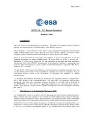
GSC Sentinel-2 PDGS STBDIssue 1 Revision 2 (draft) - 25.07.2010GMES-GSEG-EOPG-TN-09-0031page 35 of 603.4.2 PROCESSING RESOURCES ESTIMATIONThe processing activities of only one satellite are considered.The budget estimations consist in an evaluation of number of needed resources allowing torespect the delivery time constraints defined in section 3.4.2, according to the benchmarks(cf. Section 3.2) and the parallelisation opportunities of each Processing Step (recalled inSection 3.3). Assuming a linear scalability of the performance with the hardware as justifiedin 3.3.3, the number of resources (in CPU-units) will be computed as:Resources = (Scaled Benchmark time / Timeliness constraints) + Margins (%)With the following timeliness constraints: Front-End Processing: T FE = downlink-time Bulk-Processing: T BP = 100 minutesAssuming a linear relationship with the data volumes, the Reference Benchmark timeswill be scaled from the reference times by the actual volume of data to be processed withrespect to the reference datastrip volume of 57Gbytes.3.4.3 RE-PROCESSING RESOURCES ESTIMATIONThe estimation of the number of CPUs dedicated to re-processing has been made under theassumption that the data corresponding to X time shall be reprocessed up to Level-1C in 2times X (e.g. 2 months to re-process 1 month of data).Re-processing is based on the Level-0 data already processed, consolidated and archivedthen there is no need to allocate computing resources to the Level-0 processing.3.4.4 PROCESSING RESOURCES ESTIMATION WITH BOTH SATELLITESIn the previous paragraphs only the data acquired and downlinked by one satellite havebeen considered for the estimations.When both satellites will be operational, the computing resources shall be doubled to facethe doubled data volume except if some optimization in the processing time management isfound.The rationale of this scenario is fundamentally equal to Scenario 0 - one centre receivingand processing the entire amount of data, no difference between RT, NRT and Nominal dataprocessing time - but both satellites are considered and slight differences therefore arise.One satellite has an orbit period of 100 minutes.The second satellite will follow the same orbit of the first satellite with a constant phasing of180° (as showed in figure 13), i.e. 50 minutes of delay.In terms of imaging/downlink cycle, the combination of this 180° phase difference on theorbit and Earth rotation. This allows reaching the 5 days of repetitively required by themission.ESA UNCLASSIFIED – For Official Use© ESAThe copyright of this document is the property of ESA. It is supplied in confidence and shall not be reproduced, copied orcommunicated to any third party without written permission from ESA.

GSC Sentinel-2 PDGS STBDIssue 1 Revision 2 (draft) - 25.07.2010GMES-GSEG-EOPG-TN-09-0031page 36 of 60Figure 13: Sentinel-2A and Sentinel-2BIt is then assumed that data downlink will take place with 50 minutes of difference.The following rationale is adopted.Sentinel-2A downlinks on board data to the unique station at first.If all Sentinel-2A data are processed in 50 minutes, when Sentinel-2B transmits its on boarddata, the CPUs of the station will have completed S2A data processing and will be availableto process Sentinel-2B data.As shown by the chronogram of the following figure, the timeliness of the end-to-endproduction for each satellite will be lowered by 50 minutes.S2Adownlink20 min40 minS2Bdownlink60 min80 minS2Adownlink100 min120 minX CPUL0 generation (S2A)L0 generation (S2B)L0 generation (S2A)Y CPUL0 consolidation + L1 processing (S2A)L0 consolidation + L1 processing (S2B)Figure 14: Chronogram of the Scenario with 2 satellites3.4.5 SCENARIO-0 BUDGET ESTIMATIONS3.4.5.1 AssumptionsIn this simplified scenario, the resources necessary to globally process all the data areestimated assuming a simple and ideal case where all data were received and processed inone unique centre.Although not a realistic scenario, it has been considered to describe the rationale andprovide preliminary processing budget estimates.It assumes a regular pattern of data downlinks occurring once per orbit, each onecorresponding to the recovery on-ground of an average MSI datastrip identical to the oneESA UNCLASSIFIED – For Official Use© ESAThe copyright of this document is the property of ESA. It is supplied in confidence and shall not be reproduced, copied orcommunicated to any third party without written permission from ESA.

GSC Sentinel-2 PDGS STBDIssue 1 Revision 2 (draft) - 25.07.2010GMES-GSEG-EOPG-TN-09-0031page 37 of 60used for the benchmarks, i.e. an MSI acquisition of 6640 km along-track over the 290 kmswath corresponding to:- An overall MSI observation time of 16.66 minutes at an effective data supply rate of a490 Mbps;- An overall downlinked data volume of 57 GBytes ( 16.66 x 60 x 490 10 6 / 8 / 2 30 ) ofcompressed data;- A downlink time T FE = 16.66 * 490 Mbps / 520 Mbps ≈ 15.7 minutes.3.4.5.2 Processing Budget for One SatelliteThe dimensioning of the nominal processing under Scenario-0 is summarised in thefollowing table:Scenario 0(nominal processing)Front-End Processing(in real-time during the 15.7 minutesdownlink)Bulk-Processing(within 100 minutes)MethodCPU-units = 0.72 * 60 / 15.7 +15% 4CPU-units = 101.2 * 60 / 100 +15% 70Total resources 743.4.5.3 Processing Budget for Two SatellitesThe dimensioning for the nominal processing with two satellites under Scenario-0 issummarised in the following table:Scenario 0(2 satellites)Front-End Processing(in real-time during the 15.7 minutesdownlink of each spacecraft)Bulk-Processing(within 50 minutes)MethodCPUunitsCPUunitsCPU-units = 0.72 * 60 / 15.7 +15% 4CPU-units = 101.2 * 60 / 50 +15% 140Total resources 144ESA UNCLASSIFIED – For Official Use© ESAThe copyright of this document is the property of ESA. It is supplied in confidence and shall not be reproduced, copied orcommunicated to any third party without written permission from ESA.

GSC Sentinel-2 PDGS STBDIssue 1 Revision 2 (draft) - 25.07.2010GMES-GSEG-EOPG-TN-09-0031page 38 of 603.4.5.4 Re-processing BudgetThe dimensioning for the re-processing under Scenario-0 is summarised in the followingtable:Scenario 0(re-processing)Bulk-Processing(within 200 minutes)MethodCPUunitsCPU-units = 101.2 * 60 / 200 +15% 35Total resources 353.4.6 SCENARIO-1 BUDGET ESTIMATIONS3.4.6.1 AssumptionsThis scenario is based on the simulations reported in [RD-04]. In this study, an exampleCGS network of four ground-stations is assumed, composed of:CGS-1: Kiruna in Northern Sweeden; CGS-2: Svalbard (used only for the blind orbits of Kiruna) in Norway; CGS-3: Prince Albert in Northern Canada; CGS-4: Maspalomas in the Canary Islands (Spain);The study details the instrument observation and downlink times at every orbit of the repeatcycle, associating the overall imaged and downlinked data volume as well as the stationcontact times with every station.Based on the PDGS processing logic imposing a fixed amount of time (100 minutes) toprocess all the downlinked data, the worst-case considered for the budget estimationcorresponds to the largest downlink at each station over the cycle.A scaling has been applied on the simulated downlink volumes to consider: The new MSI data supply rate of 490 Mbps instead of the original 440 Mbps rateassumed in [RD-04], i.e. an increase ratio of (490/440). The volume estimations reported in [RD-04] in Gbit units are to be interpreted with1Gbit = 10 9 bits, implying a factor of (2 27 /10 9 ) for their transcriptions in GBytes as perthe conventions taken in this document.The normalisation factor is computed as a simple volume ratio with respect to the referencebenchmark datastrip size of 57GBytes. It will be used as scaling factor to the benchmarktime on the assumption of a processing time directly proportional to the size of the datastrip.ESA UNCLASSIFIED – For Official Use© ESAThe copyright of this document is the property of ESA. It is supplied in confidence and shall not be reproduced, copied orcommunicated to any third party without written permission from ESA.

GSC Sentinel-2 PDGS STBDIssue 1 Revision 2 (draft) - 25.07.2010GMES-GSEG-EOPG-TN-09-0031page 39 of 60StationDownlink Time(minutes)Downlink volume(GBytes)Normalisation Factorto the BenchmarkCGS-1 15.87 54.30 95.26%CGS-2 11.91 40.76 71.46%CGS-3 15.82 54.16 95.02%CGS-4 15.78 54.01 94.75%As indicated in the table, the downlink data volume of the worst-case orbit identified forevery station is not very different from the Reference Orbit Data Volume used in Scenario-0.It also implies that the required dimensioning of every processing station will behomogeneous to a large extent.3.4.6.2 Processing Budget for One SatelliteThe dimensioning of the nominal processing under Scenario-1 is summarised in thefollowing table:Scenario 1(nominal processing)Front-End Processing(in real-time during downlink)in CPU-unitsBulk-Processing(within 100 minutes)in CPU-unitsCGS-1 CGS-2 CGS-3 CGS-44 4 4 468 51 68 68Total resources 72 55 72 723.4.6.3 Processing Budget for Two SatellitesThe dimensioning for the nominal processing with two satellites under Scenario-1 issummarised in the following table:Scenario 1(2 satellites)Front-End Processing(in real-time during downlink)in CPU-unitsCGS-1 CGS-2 CGS-3 CGS-44 4 4 4ESA UNCLASSIFIED – For Official Use© ESAThe copyright of this document is the property of ESA. It is supplied in confidence and shall not be reproduced, copied orcommunicated to any third party without written permission from ESA.

GSC Sentinel-2 PDGS STBDIssue 1 Revision 2 (draft) - 25.07.2010GMES-GSEG-EOPG-TN-09-0031page 40 of 60Bulk-Processing(within 50 minutes)in CPU-units135 102 135 135Total resources 139 106 139 1393.4.6.4 Re-processing BudgetThe dimensioning presented here for the re-processing does consider the potential usage ofthe idle times of the resources dimensioned for the nominal processing which could be usedfor re-processing during the station blind orbit periods.The dimensioning for the re-processing under Scenario-1 is summarised in the followingtable:Scenario 1(re- processing)Bulk-Processing(within 200 minutes)in CPU-unitsCGS-1 CGS-2 CGS-3 CGS-434 26 34 34Total resources 34 26 34 34ESA UNCLASSIFIED – For Official Use© ESAThe copyright of this document is the property of ESA. It is supplied in confidence and shall not be reproduced, copied orcommunicated to any third party without written permission from ESA.

GSC Sentinel-2 PDGS STBDIssue 1 Revision 2 (draft) - 25.07.2010GMES-GSEG-EOPG-TN-09-0031page 41 of 604 DATA VOLUMES ANALYSIS4.1 AssumptionsThe dataflows of a single satellite have been considered in this analysis. All volumefigures shall be doubled to take into account the dual spacecraft constellation.The volume estimations are based on the following assumptions:- The cloud free Level-1C volume is 1/3 of the total Level-1C volume;- Europe data (land + Mediterranean sea) represents 7.5% of the total amount of imageddata.- All the level 1 volumes are intended in JPEG2000 lossless format (image coded inaverage on 7bits/pixel/band which means compression rate of 2.3)4.2 Reference Scenario for the Volumes AnalysisThe global PDGS is a distributed system, federating several stations and centres withdifferent functions and roles contributing to the overall system performance.For all analysis related to data volumes, the baseline operation scenario described in [RD-02] is used as reference and applied on the four ground stations network defined in [RD-04]composed of:CGS-1: Kiruna in Northern Sweeden; CGS-2: Svalbard (used only for the blind orbits of Kiruna) in Norway; CGS-3: Prince Albert in Northern Canada; CGS-4: Maspalomas in the Canary Islands (Spain);The following figure shows this configuration of the PDGS.ESA UNCLASSIFIED – For Official Use© ESAThe copyright of this document is the property of ESA. It is supplied in confidence and shall not be reproduced, copied orcommunicated to any third party without written permission from ESA.

GSC Sentinel-2 PDGS STBDIssue 1 Revision 2 (draft) - 25.07.2010GMES-GSEG-EOPG-TN-09-0031page 42 of 60Figure 15: PDGS Reference ConfigurationThe four stations (CGS-1, CGS-2, CGS-3 and CGS-4) have been chosen merely as anexample. As indicated in the schema and detailed in [RD-02], four different types of centrehave been distinguished according to their functions:- The CGS (Core Ground Station) has two possible configurations:• Light, with data reception role: data reception from satellite, processing up to Level-0 and relaying level-0 received data to the PAC-1.• Full, with combined data reception and data centre roles: data reception fromsatellite, processing up to Level-1C and data dissemination.- Two PACs (PAC-1 and PAC-2), each one holding a collocated LTA service functionensuring long-term data preservation in full redundancy of all Level-0, Level-1B andLevel-1C data. In addition the two PACs are configured differently as regarding their midtermrole:• PAC-1 includes a processing chain configuration to process all CGS-4 circulatedacquisitions and perform medium-term reprocessing operations on a 3 monthslevel-0 archive. It is additionally sized for on-line publishing of one year of cloudfreelevel-1C data collected from all stations.• PAC-2 is sized for on-line publishing of one year of European coverage datasupplied regularly by CGS-1/2/3 and by the PAC-1 for CGS-4 data.ESA UNCLASSIFIED – For Official Use© ESAThe copyright of this document is the property of ESA. It is supplied in confidence and shall not be reproduced, copied orcommunicated to any third party without written permission from ESA.

GSC Sentinel-2 PDGS STBDIssue 1 Revision 2 (draft) - 25.07.2010GMES-GSEG-EOPG-TN-09-0031page 43 of 60Two more centres, the MPAC – Mission Performance Assessment Centre – and the PDMC– Payload Data Management Centre – have been identified in [RD-02] but their functionsare not further recalled here because these two centres have no significant role in thecurrent analysis of the circulated and archived data.The following table details de configuration of each centre in terms of implemented functions(processing, archiving), and the data circulated between centres.Centrereceptionfrom:Data-Circulationtransmission to:NominalProcessingOn-LineArchiveOff-Line(LTA)Data-Access(Server)CGS-1CGS-2CGS-3SatellitePAC-1(Level-0/1C)PAC-2(Level-0/1B)CGS-4 Satellite PAC-1 (Level-0)PAC-1PAC-2MPACCMCCGS-4(Level-0)CGS-1/2/3(Level-0/1C)PAC-2(Level-1B)CGS-1/2/3(Level-0/1B)PAC-1(Level-1C)CGS/PACs(Cal/ValLevel-0/1A/1B/1C)MetadataonlyPAC-2(Level-1C,CGS-4 Level-0/1B)PAC-1(CGS-1/2/3Level-1B)N/AESA UNCLASSIFIED – For Official UseLevel-0/1A/1B/1CLevel-0/1A/1Bfor 1 monthLevel-1C for1 monthLevel-0 Level-0 for 1monthLevel-1A/1B/1C+Reprocessing+HostedProcessingNoneLevel-1A/1B/1Climited forpurposeCGS-4Level-1A/1Bfor 1 monthLevel-1C for1 monthCloud freeglobal Level-1C for 1 yearLevel-0 for 3monthsEuropeLevel-1C for1 yearLevel-0/1A/1B/1Climited forpurpose© ESAThe copyright of this document is the property of ESA. It is supplied in confidence and shall not be reproduced, copied orcommunicated to any third party without written permission from ESA.N/AN/ALevel-0/1B/1C for12 yearsLevel-0/1B/1C for12 yearsN/AN/A None N/A NTable 6: Product-Data Circulation Archiving ScenarioIn this example CGS-4 is a CGS in light configuration and transmits to the PAC-1 all theLevel-0 products it generates for higher level production and products dissemination tousers.YNYYN

GSC Sentinel-2 PDGS STBDIssue 1 Revision 2 (draft) - 25.07.2010GMES-GSEG-EOPG-TN-09-0031page 44 of 60“Europe Level-1C” products comprise both cloudy and cloud-free tiles; considering thatEurope has a quite limited geographical extension and that it is the main target of themission, Level-1C products over Europe follow a dedicated archiving cycle and are then keptavailable to user for a longer period than other Level-1C products.The products associated to the average datastrip of 290km large and 6640km long have thedata volumes indicated in the following table:Type of productData Volume(GBytes)Level-0 57Level-1A 89,67Level-1B 87,07Level-1C 87,07Data volumes have been estimated assuming that:- All Level-1 products are compressed in JP2K lossless (image coded in average on7bits/pixel/band which means compression rate of 2.3);- Europe data are distributed across the 4 Core Ground Stations following the samepercentage of the overall onboard data downlink (shown in Figure 16 and estimated fromthe tables of [RD-04]).Data repartition over the 4 stations17%27%45% CGS-1CGS-2CGS-3CGS-411%Figure 16: distribution across the Core Ground Station of the overall downlinked dataESA UNCLASSIFIED – For Official Use© ESAThe copyright of this document is the property of ESA. It is supplied in confidence and shall not be reproduced, copied orcommunicated to any third party without written permission from ESA.

GSC Sentinel-2 PDGS STBDIssue 1 Revision 2 (draft) - 25.07.2010GMES-GSEG-EOPG-TN-09-0031page 45 of 60Therefore, one satellite produces the following Level-0 and Level-1C data volumes (inGBytes):CGS-1 CGS-2 CGS-4 CGS-3 All StationsAverage daily volume of Level-0 366,80 89,66 138,57 220,08 815,10Average daily volume of Level-1Bor Level-1CAverage monthly volume ofLevel-0Average monthly volume ofLevel-1B or Level-1C560,29 136,96 211,66 336,17 1245,0811003,85 2689,83 4157,01 6602,31 24453,0016808,61 4108,77 6349,92 10085,16 37352,46Table 7: Data Volumes generated per product-type and Ground Station (GBytes)4.3 Data Circulation Budget EstimationsCirculation data rate has been derived as follows:Data-rate= DataVolume(T)/TWhere DataVolume(T) is the sum of the data to be transmitted during the period T.The table sums up the exchanges detailed in Table 6. Values in the table refer to an averagerequired data-rate and are expressed in Mebibit per second (Mib/s).FromCGS-1CGS-2CGS-3CGS-4PAC-1PAC-2ToPAC-1 87.9 21.5 33.2 52.7 98PAC-2 87.9 21.5 52.7 151.3Table 8: Estimated Circulation Data Rates (Mib/s)Note: the physical mechanism for data exchange (via media or digital networks) will bedefined from a cost/technical trade-off amongst available solutions. The goal is to make useof digital networks as much as possible. However, looking at the overall throughput required,a complementary circulation via media may be considered. It is highlighted that theoperation concept regarding data circulation imposes little requirements on the end-to-endlatency, but imposes a strong sustained throughput. Hence circulation via network or mediawill both be compatible with this mode of operation.ESA UNCLASSIFIED – For Official Use© ESAThe copyright of this document is the property of ESA. It is supplied in confidence and shall not be reproduced, copied orcommunicated to any third party without written permission from ESA.

GSC Sentinel-2 PDGS STBDIssue 1 Revision 2 (draft) - 25.07.2010GMES-GSEG-EOPG-TN-09-0031page 46 of 60Customarily, the physical network bandwidth is dimensioned to the double of the estimateduseful data rate so as to ensure a correct functioning of this critical component. For example,the physical network bandwidth necessary for the circulation from CGS-1 to PAC-1 would bedimensioned to about twice 87.9 Mib/s i.e. 175 Mib/s for a correct functioning.4.3.1 DATA CIRCULATION IMPACTS ON THE PROCESSING TIMEALLOCATIONIn the scenarios analysis, data processing and data circulation have been completelydecoupled therefore in the budget allowing assessing the duration for data processing thereis no allocation to the data transfer time from the Ground station to the processing centre.This choice is justified by the assumption that data reception and data processing should begenerally collocated. Indeed, n these scenarios, only the data received by the CGS-4 areprocessed by the remote PAC-1 (these data should not include NRT data), for other CGSthe processing is collocated.Considering the circulation data rate estimated in §4.2, one average orbit is transferred fromthe CGS-4 centre to the PAC-1 in:T transfer = DataVolume / DataRate ≈ 7,4 hoursDepending of the actual data transfer bandwidth available, this additional latency should betaken into account in the overall sizing of the sink PAC, to consider the reduced time budgetleft for Level-1C processing to meet the 24 hours end-to-end requirement from sensing.ESA UNCLASSIFIED – For Official Use© ESAThe copyright of this document is the property of ESA. It is supplied in confidence and shall not be reproduced, copied orcommunicated to any third party without written permission from ESA.

GSC Sentinel-2 PDGS STBDIssue 1 Revision 2 (draft) - 25.07.2010GMES-GSEG-EOPG-TN-09-0031page 47 of 604.4 Data Archiving BudgetIn the analysis of the data volumes to archive only one satellite has be considered. All thevalues shall then be doubled to take into account the second satellite also.The following table gathers the results of the archive volumes for each centre (in Tera-Byte):Data typeCGS-1CGS-2CGS-3CGS-4PAC-1PAC-2LTA3 months of Level-0 71,641 year of Level-1C cloud free(global) 131,321 year Level-1C (Europe) 32,831 month of global Level-1C 36,481 month of Level-0 10,75 2,63 6,45 4,061 month of Level-1A 16,90 4,13 10,14 6,391 month of Level-1B 16,41 4,01 9,85 2,891 month of Level-1C 16,41 8,02 19,7012 years of Level-0 3438,7012 years of Level-1B 5252,6912 years of Level-1C 5252,69Total by centre 60,48 18,80 46,14 4,06 248,71 32,83 13944,08Table 9: Data Archiving BudgetIn the table the volumes corresponding to only one Long Term Archive are indicatedbecause the LTA in PAC-1 and the LTA in PAC-2 are identical.ESA UNCLASSIFIED – For Official Use© ESAThe copyright of this document is the property of ESA. It is supplied in confidence and shall not be reproduced, copied orcommunicated to any third party without written permission from ESA.

GSC Sentinel-2 PDGS STBDIssue 1 Revision 2 (draft) - 25.07.2010GMES-GSEG-EOPG-TN-09-0031page 48 of 604.5 Volumes of Processing DataThe “processing data volume” comprises not only the Mission data - compressed oruncompressed according to the particular Processing Step - and the Satellite Ancillary databut also all the auxiliary data necessary for their processing (DEM, reference images, etc).Hence, the processing data volume is defined for each Processing Step as the sum of theinput, output and auxiliary data volumes.Hereafter, the estimation of the Processing Data Volume for each Processing Stepconsidering the Reference Orbit Data Volume defined in § 4.3.2.2.Table 6 indicates for each Processing Step the data necessary for the processing.Input data Processing Output data Auxiliary dataMSI TM + HK TM Ana TM GSPGSPGSP+LR Images(5 bds)GSP, QL5bdsGSP, QL5bdsDatation& LR extractionInitLocInv,QL & TQ masksCloudMasks InvJP2K comprLR imagesQL5bds+TQmasksGSP, QL5bds,Cloud MasksGSP, QL4bdscompressedDEMLevel-0 ConsolidatedMetadata+GSP Init Loc Prod MetadataGSP Decomp Level-1ALevel-1A RadioS2 (part 2) Level-1A+Level-1A+ GeoS2 Level-1B DEM+ Ref ImageLevel-1B Resample Level-1C DEMLevel-1CJP2K comprLevel-1CcompressedLevel-1C GeneratedTable 10: Processing Data VolumesESA UNCLASSIFIED – For Official Use© ESAThe copyright of this document is the property of ESA. It is supplied in confidence and shall not be reproduced, copied orcommunicated to any third party without written permission from ESA.

GSC Sentinel-2 PDGS STBDIssue 1 Revision 2 (draft) - 25.07.2010GMES-GSEG-EOPG-TN-09-0031page 49 of 60The volumes of metadata are considered negligible.The volumes of DEM, LR images, and Quicklook images have been estimated consideringthe reference segment size (290km x 6640 km), their resolution and their coding:Type of dataGeometricalResolution (m)Coding (bits)Volume (Gbit)DEM 60 16 7.97LR images (each band) 320 12 0.21(x 5 bands)QL images (each band) 320 12 0.21(x 4 bands)Ref Image 10 16 286.94In the following figure the graphical representation of the evolution of the processing datavolume across the production steps. The processing data volume of the figure below is thesum of the Input, Output and Auxiliary data indicated for each processing step in Table 8.Level-1 processing is very demanding in terms of data volume allocation because imagedata are uncompressed and the necessary auxiliary data have big volumes (especially DEMand Reference images).Total volume needed500,00450,00Processing Volume (Gbyte)400,00350,00300,00250,00200,00150,00100,0050,000,00Ana TMDatation & LR extractionInitLocInv, QL & TQ masksCloud Masks InvJP2K comprLevel 0Init Loc ProdDecompRadio S2Geo S2ResampleJP2K comprLevel1CProcessing stepESA UNCLASSIFIED – For Official Use© ESAThe copyright of this document is the property of ESA. It is supplied in confidence and shall not be reproduced, copied orcommunicated to any third party without written permission from ESA.

GSC Sentinel-2 PDGS STBDIssue 1 Revision 2 (draft) - 25.07.2010GMES-GSEG-EOPG-TN-09-0031page 50 of 604.6 Data Dissemination BudgetAccording to the Data Access Portfolio document, an estimate of the data volumes requiredyearly by the users has been conducted (cf. [RD-02]). It is underlined that the current versionof the DAP-R does not cover explicitly the Sentinel-2 image and thus all the requirementsand constrains have been extrapolated considering the service requirement relevance toSentinel-2 type of data.Starting from the areas of interest explicitly mentioned by the Services in DAP-R, theaveraged values of satellite data requested have been calculated. Nominal data is foreseento be delivered systematically on predefined task while the request for NRT data is notdeterministic (even if some possible NRT scenarios could be anticipated).PDGSNRT DataNRTNominal DataMARINENominal DataSECURITYNominal NominalRepositoryNominal DataNominal DataEMERGENCYLANDGMES SERVICESTaking into account the statistical occurrence of natural and anthropic hazards an averageof 450 events yearly during the last 10 years have occurred affecting an area of 100.000squared km for each disaster. A possible request of 150 NRT data scene charter activationsper year has been assumed as plausible for a total of 1000 GBytes of NRT data yearly. Amargin of 30% in the amount has been introduced for taking into account possible mistakesin the submitted orders.SERVICESNOMINAL[GBytes]NRT[GBytes]TOTAL[GBytes]LAND 1550 0 1550EMERGENCY 1600 1000 2600SECURITY 61 12 73MARINE 25 50 75TOTAL 3236 1062 4298Table 11: GMES Services Sentinel-2 Annual Data VolumeESA UNCLASSIFIED – For Official Use© ESAThe copyright of this document is the property of ESA. It is supplied in confidence and shall not be reproduced, copied orcommunicated to any third party without written permission from ESA.

GSC Sentinel-2 PDGS STBDIssue 1 Revision 2 (draft) - 25.07.2010GMES-GSEG-EOPG-TN-09-0031page 51 of 60The results of the analysis based on a year of possible supply scenario are shown in Table11. Thus, about 24% of the overall amount intended to the GMES services is foreseen to bedelivered in NRT.In terms of scenes (290x290 km), the number of requested images needed to cover theGMES interested areas, is thus around 1000 per year, in terms of tiles (100 x 100 km) it isalmost nine times greater.24%76%NominalNRTFigure 17: Nominal/NRT Product Usage ExpectationsThe data-access requirement analysis reported in [RD-02] Annex-A has further underlined asubstantial expected growth from the DAP/R extrapolated estimates justified by the veryopen data-policy assumed for Sentinel-2. As a matter of fact, the recent experience ofLANDSAT open archive suggests that the overall annual amount of images datadownloaded should be 100 times greater than the ones extrapolated from DAP/R andresulting to an overall yearly estimate of 400 TBytes.The resulting average required data dissemination bandwidth apportioned between NRT(24%) and nominal (76%) access requirements is reported in the following table. The dataratefigures refer to an average useful data-rate and are expressed in Mebibit per second(Mib/s).Data AccessRequirementsYearly VolumeAverage SustainedData-RateNRT 96 TBytes/year 25.5 Mib/sOther 304 TBytes/year 80.9 Mib/sTotal 400 TBytes/year 106.4 Mib/sTable 12: Estimated Dissemination Throughput RequirementCustomarily, the physical network bandwidth will be dimensioned to the double of theestimated useful data rate so as to ensure a correct functioning. Assuming a regulardistribution of the requests along time, the dimensioned physical network bandwidth tosupport the overall dissemination would result to about 210 Mib/s.ESA UNCLASSIFIED – For Official Use© ESAThe copyright of this document is the property of ESA. It is supplied in confidence and shall not be reproduced, copied orcommunicated to any third party without written permission from ESA.

GSC Sentinel-2 PDGS STBDIssue 1 Revision 2 (draft) - 25.07.2010GMES-GSEG-EOPG-TN-09-0031page 52 of 605 HARDWARE ARCHITECTURE PRINCIPLESThis chapter provides an overview of the generic principles for the processing/archivingsystem hardware architecture design.The material means can be distinguished in the following categories:o Computation means, assured operated by a computer cluster: this physically groupsthe different processing means in compact frames offering an adapted connectivityand centralized administration means.o Online storage means, deployed around a SAN (Storage Area Network) andcomposed by disk arrays.o Archiving and backup means.The group of servers is interconnected via an Ethernet network offering a bandwidth varyingfrom 1 Gbps to 10Gbps according to the needs.Figure 18 : Logical architectureThe figure above outlines the possible architecture of one centre; the schema is notrepresentative of the number of real platforms composing the network or of the number ofphysical interconnections.ESA UNCLASSIFIED – For Official Use© ESAThe copyright of this document is the property of ESA. It is supplied in confidence and shall not be reproduced, copied orcommunicated to any third party without written permission from ESA.

Local Area NetworkGSC Sentinel-2 PDGS STBDIssue 1 Revision 2 (draft) - 25.07.2010GMES-GSEG-EOPG-TN-09-0031page 53 of 60It allows the interconnection between the servers of the different units or subsystems, i.e.:o The exchanges between the servers of the computer clustero The exchanges between the operator terminals and the computer cluster,It allows also the links with the centre infrastructure (from dislocated operator terminals) andthe exchanges between different centres.Computer clusterIt is a BladeCenter comprising several server-blades. The frame offer to servers theinterconnection resources they need (network, supply).These blades have identical material characteristics and they are allocated:o Statically at one subsystem start - one blade having the opportunity of hosting severalsubsystems,o Dynamically for image processing algorithms.Up-to-date information about the computation power of the most recent hardwareconfiguration can be found on the website SPEC.org.Benchmarked values presented in chapter 4 have been estimated using IBM BladeCenterHS21 (Intel Xeon E5430) which has come out in winter 2008 (Base: 21.1, peak: 24.1Mflops). The latest Blade Center dating summer 2009 has much higher performancesassuring for example a base value 36.3 Mflops and a peak value of 38.9 Mflops (IBMBladeCenter HS22 (Intel Xeon X5560)).Furthermore, better processing time can be expected thanks to technological evolutions.Storage Area NetworkIt allows the computer cluster servers to access via a Fibre Channel network to remotecomputer storage devices (such as disk arrays, tape libraries) as if these devices werelocally attached to the operating system (in terms of data rate I/O). Each server has an HBAcard allowing it to access to the disk volumes which are shared with the other servers.Disk arraysThe disk array hosts unit or subsystem data. These disks have a RAID array configurationoffering both redundancy and the performances needed for supporting the required I/Orates. Volumes are shared between servers via a high performance clustered file system.Storage capacities are dimensioned according to each centre needs.Archive and backup meansThey can be composed of a LTO libraries exclusively used by the archive subsystem and bythe subsystem charged of the backup. This library is managed by a server that is external tothe integrated computer cluster.Storage capacities are dimensioned according to each centre needs.ESA UNCLASSIFIED – For Official Use© ESAThe copyright of this document is the property of ESA. It is supplied in confidence and shall not be reproduced, copied orcommunicated to any third party without written permission from ESA.

GSC Sentinel-2 PDGS STBDIssue 1 Revision 2 (draft) - 25.07.2010GMES-GSEG-EOPG-TN-09-0031page 54 of 606 CONCLUSIONThis document has described the Sentinel-2 PDGS technical budget offering a preliminarydimensioning that, even if it needs to be refined by the PDGS prime contractor, allowshighlighting the bottlenecks and the greatest difficulties but also showing the feasibility of thesystem.The Nominal and NRT timeliness constraints are finally less problematic than it seemed atthe beginning of the analysis.The main difficulties are linked to the huge data volume to manage for processing,circulation, dissemination and archive.Considered the instrument complex architecture, complicated algorithms shall be applied forthe corrections on ground and they shall foresee a high level of parallelisation to meet thetimeliness requirements. Nowadays solutions exist to solve this point thus, under this aspect,the PDGS team is confident about system feasibility.The federative configuration is the main bottleneck of Sentinel-2 PDGS development.The amount of data to circulate, distribute and archive has no precedents and it constitutes atechnological challenge that is without any doubts solvable with nowadays resources andthat in the future will be for sure even easier to cope with.ESA UNCLASSIFIED – For Official Use© ESAThe copyright of this document is the property of ESA. It is supplied in confidence and shall not be reproduced, copied orcommunicated to any third party without written permission from ESA.