- Page 1:
GRAVITATIONAL WAVES
- Page 4 and 5:
c IOP Publishing Ltd 2001All righ
- Page 6 and 7:
viContents4 Astrophysics of gravita
- Page 8 and 9:
viiiContents11.3 Gravitational wave
- Page 10 and 11:
xContents16.5 Cosmological perturba
- Page 13 and 14:
PrefaceGravitational waves today re
- Page 15 and 16:
2 Gravitational waves, theory and e
- Page 17 and 18:
4 Gravitational waves, theory and e
- Page 19 and 20:
6 Gravitational waves, theory and e
- Page 21 and 22:
8 Gravitational waves, theory and e
- Page 23 and 24:
10 Gravitational waves, theory and
- Page 26 and 27:
SynopsisGravitational waves and the
- Page 28 and 29:
Chapter 2Elements of gravitational
- Page 30 and 31:
Using the TT gauge to understand gr
- Page 32 and 33:
Interaction of gravitational waves
- Page 34 and 35:
Analysis of beam detectors 21This d
- Page 36 and 37:
Exercises for chapter 2 232. Show t
- Page 38 and 39:
Gravitational-wave detectors 25indi
- Page 40 and 41:
Gravitational-wave observables 27th
- Page 42 and 43:
The physics of interferometers 29
- Page 44 and 45:
The physics of interferometers 31Dr
- Page 46 and 47:
The physics of interferometers 33Fi
- Page 48 and 49:
The physics of resonant mass detect
- Page 50 and 51:
The physics of resonant mass detect
- Page 52 and 53:
A detector in space 39LISA has been
- Page 54 and 55:
Gravitational and electromagnetic w
- Page 56 and 57:
Chapter 4Astrophysics of gravitatio
- Page 58 and 59:
Sources detectable from ground and
- Page 60 and 61:
Sources detectable from ground and
- Page 62 and 63:
Sources detectable from ground and
- Page 64 and 65:
Variational principles and the ener
- Page 66 and 67:
Variational principles and the ener
- Page 68 and 69:
Practical applications of the Isaac
- Page 70 and 71:
Exercises for chapter 5 57(f)This s
- Page 72 and 73:
Expansion for the far field of a sl
- Page 74 and 75:
Application of the TT gauge to the
- Page 76 and 77:
Application of the TT gauge to the
- Page 78 and 79:
Application of the TT gauge to the
- Page 80 and 81:
Application of the TT gauge to the
- Page 82 and 83:
6.4.1 Mass-quadrupole radiationEner
- Page 84 and 85:
Chapter 7Source calculationsNow tha
- Page 86 and 87:
The r-modes 73As we mentioned in ch
- Page 88 and 89:
The r-modes 75instability. In an id
- Page 90 and 91:
The r-modes 77Table 7.1. Gravitatio
- Page 92 and 93:
The r-modes 79evolution turns out t
- Page 94 and 95:
ReferencesWe have divided the refer
- Page 96 and 97:
References 83[19] van der Klis M 19
- Page 98 and 99:
Solutions to exercises 85For this p
- Page 100 and 101:
Solutions to exercises 87The gauge
- Page 103 and 104:
Chapter 8Resonant detectors for gra
- Page 105 and 106:
Sensitivity and bandwidth of resona
- Page 107 and 108:
8.2 Sensitivity for various GW sign
- Page 109 and 110:
Sensitivity for various GW signals
- Page 111 and 112:
Recent results obtained with the re
- Page 113 and 114:
Discussion and conclusions 101Figur
- Page 115 and 116:
Chapter 9The Earth-based large inte
- Page 117 and 118:
Introduction 105Figure 9.1. The sim
- Page 119 and 120:
h(sqrt(1/Hz))10 −610 −810 −10
- Page 121 and 122:
18.5 cmThe SA suspension and requir
- Page 123 and 124:
A few words about the Low Frequency
- Page 125 and 126:
Conclusion 113Figure 9.7. The R and
- Page 127 and 128:
Chapter 10LISA: A proposed joint ES
- Page 129 and 130:
Description of the LISA mission 117
- Page 131 and 132:
Description of the LISA mission 119
- Page 133 and 134:
Description of the LISA mission 121
- Page 135 and 136:
Description of the LISA mission 123
- Page 137 and 138:
Description of the LISA mission 125
- Page 139 and 140:
Description of the LISA mission 127
- Page 141 and 142:
Description of the LISA mission 129
- Page 143 and 144:
Description of the LISA mission 131
- Page 145 and 146:
Expected gravitational-wave results
- Page 147 and 148:
Expected gravitational-wave results
- Page 149 and 150:
Expected gravitational-wave results
- Page 151 and 152:
Expected gravitational-wave results
- Page 153 and 154:
Expected gravitational-wave results
- Page 155 and 156:
Expected gravitational-wave results
- Page 157 and 158:
Expected gravitational-wave results
- Page 159 and 160:
Expected gravitational-wave results
- Page 161 and 162:
References 149[8] Folkner W M 1998
- Page 163 and 164:
References 151[68] Miralda-Escuda J
- Page 165 and 166:
Introduction 153detect GWs with a s
- Page 167 and 168:
Testing theories of gravity 155•
- Page 169 and 170:
0Testing theories of gravity 157the
- Page 171 and 172:
Taking the scalar product we findGr
- Page 173 and 174:
Gravitational wave radiation in the
- Page 175 and 176:
Gravitational wave radiation in the
- Page 177 and 178:
Gravitational wave radiation in the
- Page 179 and 180:
Gravitational wave radiation in the
- Page 181 and 182:
The hollow sphere 169and introduced
- Page 183 and 184:
Scalar-tensor cross sections 171mon
- Page 185 and 186:
Scalar-tensor cross sections 173Tab
- Page 187 and 188:
Scalar-tensor cross sections 175Tab
- Page 189 and 190:
References 177Frossati G and Coccia
- Page 192 and 193:
Chapter 12Generalities on the stoch
- Page 194 and 195:
Introduction 183contribution to the
- Page 196 and 197:
Definitions 185The value of H 0 is
- Page 198 and 199:
Definitions 18712.2.2 The character
- Page 200 and 201:
Definitions 189or, dividing by the
- Page 202 and 203:
The overlap reduction function 191O
- Page 204 and 205:
The overlap reduction function 193T
- Page 206 and 207:
The overlap reduction function 195F
- Page 208 and 209:
Achievable sensitivities to the SGW
- Page 210 and 211:
Achievable sensitivities to the SGW
- Page 212 and 213:
Achievable sensitivities to the SGW
- Page 214 and 215:
Achievable sensitivities to the SGW
- Page 216 and 217:
Achievable sensitivities to the SGW
- Page 218 and 219:
Observational bounds 207Table 12.10
- Page 220 and 221:
equation gives immediately(ρgwρ
- Page 222 and 223:
Chapter 13Sources of SGWBHere we re
- Page 224 and 225:
Topological defects 213This correla
- Page 226 and 227:
Topological defects 215It can be sh
- Page 228 and 229:
Topological defects 217(i)A loop ra
- Page 230 and 231:
Topological defects 219• A peak n
- Page 232 and 233:
Topological defects 22113.1.2 Hybri
- Page 234 and 235:
Inflation 223Hubble radius and when
- Page 236 and 237:
Inflation 225as a first approximati
- Page 238 and 239:
Inflation 227the lower bound to the
- Page 240 and 241:
String cosmology 22913.3 String cos
- Page 242 and 243:
String cosmology 231HPre-big bangPo
- Page 244 and 245:
String cosmology 233Figure 13.6. h
- Page 246 and 247:
First-order phase transitions 23580
- Page 248 and 249:
Astrophysical sources 237which is t
- Page 250 and 251:
References 239of [71]). However, fo
- Page 252 and 253:
References 241[39] Liddle A R 2000
- Page 254:
PART 4THEORETICAL DEVELOPMENTSHerma
- Page 257 and 258:
246 Infinite-dimensional symmetries
- Page 259 and 260:
248 Infinite-dimensional symmetries
- Page 261 and 262:
250 Infinite-dimensional symmetries
- Page 263 and 264:
252 Infinite-dimensional symmetries
- Page 265 and 266:
254 Infinite-dimensional symmetries
- Page 267 and 268:
256 Infinite-dimensional symmetries
- Page 269 and 270:
258 Infinite-dimensional symmetries
- Page 271 and 272:
260 Infinite-dimensional symmetries
- Page 273 and 274:
262 Infinite-dimensional symmetries
- Page 275 and 276:
264 Infinite-dimensional symmetries
- Page 277 and 278:
266 Infinite-dimensional symmetries
- Page 279 and 280:
Chapter 15Gyroscopes and gravitatio
- Page 281 and 282:
270 Gyroscopes and gravitational wa
- Page 283 and 284:
272 Gyroscopes and gravitational wa
- Page 285 and 286:
274 Gyroscopes and gravitational wa
- Page 287 and 288:
276 Gyroscopes and gravitational wa
- Page 289 and 290:
278 Gyroscopes and gravitational wa
- Page 291 and 292:
Chapter 16Elementary introduction t
- Page 293 and 294:
282 Elementary introduction to pre-
- Page 295 and 296:
284 Elementary introduction to pre-
- Page 297 and 298:
286 Elementary introduction to pre-
- Page 299 and 300:
288 Elementary introduction to pre-
- Page 301 and 302: 290 Elementary introduction to pre-
- Page 303 and 304: 292 Elementary introduction to pre-
- Page 305 and 306: 294 Elementary introduction to pre-
- Page 307 and 308: 296 Elementary introduction to pre-
- Page 309 and 310: 298 Elementary introduction to pre-
- Page 311 and 312: 300 Elementary introduction to pre-
- Page 313 and 314: 302 Elementary introduction to pre-
- Page 315 and 316: 304 Elementary introduction to pre-
- Page 317 and 318: 306 Elementary introduction to pre-
- Page 319 and 320: 308 Elementary introduction to pre-
- Page 321 and 322: 310 Elementary introduction to pre-
- Page 323 and 324: 312 Elementary introduction to pre-
- Page 325 and 326: 314 Elementary introduction to pre-
- Page 327 and 328: 316 Elementary introduction to pre-
- Page 329 and 330: 318 Elementary introduction to pre-
- Page 331 and 332: 320 Elementary introduction to pre-
- Page 333 and 334: 322 Elementary introduction to pre-
- Page 335 and 336: 324 Elementary introduction to pre-
- Page 337 and 338: 326 Elementary introduction to pre-
- Page 339 and 340: 328 Elementary introduction to pre-
- Page 341 and 342: 330 Elementary introduction to pre-
- Page 343 and 344: 332 Elementary introduction to pre-
- Page 345 and 346: 334 Elementary introduction to pre-
- Page 347 and 348: 336 Elementary introduction to pre-
- Page 349 and 350: Chapter 17Post-Newtonian computatio
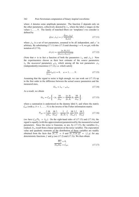
- Page 351: 340 Post-Newtonian computation of b
- Page 355 and 356: 344 Post-Newtonian computation of b
- Page 357 and 358: 346 Post-Newtonian computation of b
- Page 359 and 360: 348 Post-Newtonian computation of b
- Page 361 and 362: 350 Post-Newtonian computation of b
- Page 363 and 364: 352 Post-Newtonian computation of b
- Page 365 and 366: 354 Post-Newtonian computation of b
- Page 367 and 368: 356 Post-Newtonian computation of b
- Page 369: PART 5NUMERICAL RELATIVITYEdward Se
- Page 372 and 373: 362 Numerical relativityspite of mo
- Page 374 and 375: 364 Numerical relativityterms, of m
- Page 376 and 377: 366 Numerical relativityHere we hav
- Page 378 and 379: 368 Numerical relativityinformation
- Page 380 and 381: 370 Numerical relativityThe Palma,
- Page 382 and 383: 372 Numerical relativityHyperbolic
- Page 384 and 385: 374 Numerical relativityEinstein di
- Page 386 and 387: 376 Numerical relativityare the abi
- Page 388 and 389: 378 Numerical relativityeach cell i
- Page 390 and 391: 380 Numerical relativityFigure 18.1
- Page 392 and 393: 382 Numerical relativity1D code [45
- Page 394 and 395: 384 Numerical relativityfunctions,
- Page 396 and 397: 386 Numerical relativityto a very a
- Page 398 and 399: 388 Numerical relativity18.5 Comput
- Page 400 and 401: 390 Numerical relativitynumerics an
- Page 402 and 403:
392 Numerical relativityinitial dis
- Page 404 and 405:
394 Numerical relativityFigure 18.2
- Page 406 and 407:
396 Numerical relativityof these re
- Page 408 and 409:
398 Numerical relativityFigure 18.4
- Page 410 and 411:
400 Numerical relativityof Einstein
- Page 412 and 413:
402 Numerical relativity18.9.5.2 Co
- Page 414 and 415:
404 Numerical relativity[23] Ashby
- Page 416 and 417:
406 Numerical relativity[101] Shapi
- Page 418 and 419:
408 Numerical relativity(Singapore:
- Page 420 and 421:
410 IndexEhlers Lagrangian, 254Eins
- Page 422:
412 Indexscalarspherical harmonics,