Georg-August-Universität Göttingen - Institut für Numerische und ...

Georg-August-Universität
Göttingen
Integrating Line Planning, Timetabling, and Vehicle
Scheduling:
A customer-oriented approach
M. Michaelis and A. Schöbel
Nr. 2008-04
Preprint-Serie des
Instituts für Numerische und Angewandte Mathematik
Lotzestr. 16-18
D - 37083 Göttingen

Integrating Line Planning, Timetabling, and
Vehicle Scheduling: A customer-oriented
approach ∗
Mathias Michaelis Anita Schöbel
March 28, 2008
Abstract
Given an existing public transportation network, the classic planning
process in public transportation is as follows: In a first step, the lines are
designed; in a second step a timetable is calculated and finally the vehicle
and crew schedules are planned. The drawback of this sequence is that the
main factors for the costs (i.e. the number of vehicles and drivers needed)
are only determined in a late stage of the planning process.
We hence suggest to reorder the classic sequence of the planning steps:
In our new approach we first design the vehicle routes, then split them to
lines and finally calculate the timetable. The advantage is that costs can
be controlled during the whole process while the objective in all three steps
is customer-oriented.
In the paper we formulate this approach, discuss the complexity of
the resulting problems, and present a heuristic which we applied within a
case-study, optimizing the local bus system in Göttingen, Germany.
1 Motivation and related literature
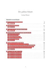
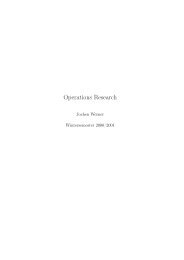
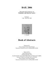
The strategic planning process in public transportation is usually divided
in the planning steps depicted in Figure 1. In this paper we are interested
in the following three steps: line planning, timetabling, and vehicle
scheduling.
To sketch these three steps, let PTN = (V, E) be a directed graph representing
the public transportation network. It consists of a set of (potential)
stops or stations V and a set of direct connections between them.
∗ This work was partially supported by the Future and Emerging Technologies Unit of EC
(IST priority - 6th FP), under contract no. FP6-021235-2 (project ARRIVAL).
1

infrastructure
lines and frequencies
timetable
vehicle routes
crew schedules
Delay−management,
Re−Scheduling,...
infrastructure
vehicle routes
lines
timetable
crew schedules
Delay−management,
Re−Scheduling,...
Figure 1: The classic planning phases in public transportation (left) compared to the
sequence used in this paper (right).
Line planning. A line l is a path in the public transportation network
PTN. The frequency fl of a line l says how often service is offered along line
l within a (given) time period I. A line concept is a set of lines together
with their frequencies.
In most research papers it is assumed that a line pool of potential lines is
already given. The goal is to choose a set of lines from the pool and to
assign frequencies to the lines chosen. Unfortunately, even the feasibility
problem (finding frequencies such that the constraints at each edge are
satisfied) is NP hard (see [Bus98, CvDZ98]).
One distinguishes between cost-oriented models (see e.g. [CvDZ98, Zwa97,
Goo04, BLL04, GvHK06]) in which the line concept has to cover a given
demand with smallest possible costs, and customer-oriented models where
a budget is given that should be used in a way that is “best” for the passengers.
Examples for customer-oriented objective functions are to maximize
the number of direct travelers ([BKZ96, Bus98]) or to minimize the traveling
time of the passengers (see [BGP05, BP05, SS06, Sch05], where the latter
two also took the time for transfers into account). Designing lines which
can compete with the private mode has been studied in [LnMO06, LMO05].
Note that [CvDZ98] already considered the vehicle schedules of later planning
steps.
There are rather few papers in which the lines are constructed during the
process of line planning. In the very first paper about line planning, Patz
([Pat25]) starts with a line for each OD pair and iteratively eliminates lines
2

y a greedy approach. A similar greedy heuristic is due to [Son77]. More
recently, [UP95] and [Qua03] suggest constructive approaches, the latter
also dealing with timetabling within the next planning step. Integration
of line planning and periodic timetabling has also been done in [LM06].
In this paper we suggest a constructive heuristic using a customer-oriented
approach.
Timetabling. Given the set of stations V and the set of vehicles F , a
timetable consists of two functions π arr : V × F → IN, π dep : V × F → IN
assigning a departure time and an arrival time to each vehicle at each
station. To avoid indices event activity networks are used in timetabling
(see [Nac94]) in which the events consist of all arrivals and departures of
all vehicles at all stations. The events are linked by edges corresponding
to three types of activities: driving activities of vehicles between stations,
waiting activities of vehicles at stations, and transfer activities to account
for passengers changing busses or trains.
We have to distinguish between periodic and aperiodic timetabling. The
latter can be efficiently solved by shortest path techniques while the former
is NP-hard (see [Nac94]). The basis for tackling periodic timetabling is the
periodic event scheduling problem (PESP) originally introduced in [SU89].
There are many extensive studies about timetabling, we refer to [Pee02,
Lie06] and references therein. Current approaches deal with integration
aspects (e.g. [LM04]) or robustness issues ([KDV07, LSS + 07, FSZ07]).
Vehicle Scheduling. If the lines and the timetable are given one can
define the trips which have to be served, i.e. the minimal pieces which have
to be operated by the same bus (usually between start and end station of a
line). For each trip we have given its start station with its departure time
and its end station with its arrival time. Two trips trip1 and trip2 can be
served by the same bus if the arrival time at the end station of trip1 plus
the time needed to drive from the end station of trip1 to the start station
of trip2 is smaller than the departure time at the start station of trip2.
The goal is to find a cost-minimal assignment between busses and trips
such that each trip is covered by exactly one bus and the schedules of all
vehicles are feasible. While the multi-depot case is NP-hard (see [BCG87]
and [PDHH06] for a comparison of different heuristics), the single-depot
case can be solved polynomially. Approaches include decomposition models
([Sah72]), assignment models ([Orl76]), transportation models ([GS78]) or
network flow models ([DP95]). An excellent survey paper dealing with bus
scheduling is [BK06], railway issues are treated in [Mar06].
Research in vehicle scheduling includes practical extensions as multiple vehicle
types (e.g. [Löb97]), route constraints (e.g.[KGS06]), or maintenance
issues. Recently, robustness issues are considered within the framework of
ARRIVAL [ARR].
3

In contrast to the approaches in the literature and to the classic planning
process in public transportation, we follow a new approach in this paper.
We start by determining the routes of the vehicles, then add a timetable
and split them to lines.
We repeat the most crucial notation that will be used throughout this text.
• A line is a path in the PTN along which service is offered.
• A timetable specifies the departure and arrival times of each vehicle
at each station.
• For the vehicle schedules we distinguish between the vehicle routes
which are given as paths in the PTN and the vehicle schedule which
assigns arrival and departure times to the routes.
Since we are looking for a periodic schedule we assume that one common
period T is given after which everything is repeated. We plan for only one
period but take the periodicity into account when evaluating our objective
function.
2 Planning an attractive transportation
system
The main idea of our new approach is to start the whole process by designing
the vehicle routes. A vehicle route is the path a vehicle drives in
the PTN given as a sequence of stops in V or as a sequence of edges e ∈ E.
The set of all routes in the final public transportation system is denoted
by U. Each vehicle route u ∈ U has a frequency fu specifying how many
trips should be offered along the route within the same planning period
and a schedule tu assigning an arrival and a departure time to each stop
of the route. It will turn out that these values (U, f, t) are sufficient as
variables, i.e, not only the vehicle schedules, but also the lines and the
timetable together with their costs and attractiveness can be determined
if U and fu, tu are known for all u ∈ U.
We remark that the routes are planned as circles such that they can be
repeated in the next period.
Let us consider the ingredients we need for the problem.
The public transportation network PTN =(V,E). For each edge
e in the PTN we determine two lengths: dbus(e) is the time a bus needs for
running between i and j, while dpriv(e) is the time needed in the private
mode i.e. by foot or by car. For most edges, dpriv(e) ≤ dbus(e). The
duration of a route is defined as the sum of all edge lengths (in the public
mode) of edges contained in the route, i.e.
dur(u) = �
dbus(e).
e∈u
4

Footpaths connecting nearby stops (e.g. on the two different sides of a
street) are also included in our model to allow passengers to walk from one
stop to another.
In our work we distinguish between stops V and locations B, where the
latter is a set of stops with the same name. Usually two stops (on either
side of a road) form a location. In a one-way street there may be locations
consisting of only one stop, whereas a location near an intersection may
consist of four stops. The reason for aggregating the stops is that the
evaluation of a public transportation system is based rather on locations
than on stops since customers do not mind on which side of a street they
depart or arrive.
Data about the potential demand. Our goal is to design an attractive
public transportation system, i.e. one that meets the demand of the
citizens. We are interested not only in improvements for existing customers
but also in attracting new customers. Hence we use an origin-destination
matrix representing the complete demand. This matrix is certainly not
based on stops. It is given due to demand regions (called cells). By assigning
cells to their closest locations we obtain an origin-destination matrix
OD ∈ ZZ |B|×|B| . (Details are given in Section 4.) In the following let us
assume that for each pair i, j ∈ B of locations the value ODij represents
the number of persons who want to travel from i to j, i.e. the potential
number of customers for this OD-pair.
Given an OD-pair of locations i, j a customer is interested in a “good” (i.e.
a fast) trip from i to j in the public transportation system. These trips
will be called passengers’ paths between i and j.
Constraints. We consider two major constraints: the costs and the
capacity of our system.
The costs of a public transportation system are mainly determined by the
number of vehicles running per day, since this number determines not only
the investment costs but also fixes the number of drivers and conductors
needed. Our budget constraint hence bounds the number of vehicles N
that we are allowed to use. Note that the number of vehicles needed
(within one period of time) can be determined by the vehicle routes and
their frequencies, namely by
� �
dur(u) · fu
number of vehicles for route u =
. (1)
T
In our construction process we take care of designing vehicle routes u with
a duration dur(u) a bit less than one time period T . In this case we obtain
fu as the number of busses necessary for route u.
There is another constraint we are taking into account: we ensure that the
space available for busses is sufficient at each of the stops. As parameters
5

we have given a capacity cap(v) indicating how many busses are allowed
to be at the stop v at the same time.
We remark that there are a lot of other constraints in practice. These
include breaks for the drivers, slack times to make the timetable more
robust and constraints for the specific shape and structure of the lines.
They can be considered when constructing the vehicle routes in the first
phase of our algorithm.
Objective function. We define the attractiveness of a public transportation
system as the average probability that a (potential) traveler
decides to use public transportation instead of the private mode.
objective function hence is
Our
max �
(2)
(i,j)∈B×B
pijODij
where ODij is the potential demand between locations i and j and pij is
the probability that a person who wants to travel between stops i and j
uses public transportation. The probability pij depends on many factors.
Talking to practitioners we decided to focus on
pwij: the average waiting time for trips from i to j and on
pdij: the travel time of public transport (compared to the travel time of
the private mode) between i and j
to determine the probability that a person decides to use public transportation
for his or her trip from i to j. The idea to compare the traveling
times in public and private mode has also been used by Laporte, Mesa and
Ortega, see [LMO05].
In the following we show in detail how to estimate pij. We start from a
solution (U, f, t) consisting of vehicle routes U with their frequencies f and
their schedules t.
We are interested in (the number and quality of) all possibilities how a
passenger can travel from i to j. Given (U, f, t) such a passenger path is
specified by
• the routes and stops it uses, and
• by the arrival and departure times of all its stops.
Note that two consecutive stops of a passenger path are either contained
in the same route or the passenger has to transfer between two vehicles.
In order to find all possible passengers’ paths we set up the timetable
graph defined by the PTN and our solution (U, f, t). This graph contains
all the relevant information for a timetable information system and allows
to determine the set of all possible passengers’ paths Pij from i to j for
each pair of locations i, j ∈ B, see [BDW07] for a recent comparison of
methods.
6

For each p ∈ Pij we collect
dep(p) = starting time at i
arr(p) = arrival time at j
dur(p) = arr(p) − start(p)
= time needed to travel from i and j using path p
We then take the best paths of this set. To this end we use the smallest
possible traveling time
dur min
ij
and fix a value λ to determine
= min dur(p)
p∈Pij
Gij = {p ∈ Pij : dur(p) ≤ λ · dur min
ij and
there does not exist a path p ′ ∈ Pij satisfying
dep(p ′ ) ≥ dep(p), arr(p ′ ) ≤ arr(p), dur(p ′ ) ≤ dur(p)} (3)
as the set of “good” passengers’ paths between i and j. With the help of
this set, we can estimate the two parameters pd and pw to estimate the
probability that a customer uses public transportation when traveling from
i to j:
pd: We compare the travel time in public transport with the travel time
using the private mode, i.e. we calculate
where public ij =
P
p∈G ij dur(c)
|Gij|
rij = private ij
public ij
denotes the average travel time in pub-
lic transportation and privateij is the travel time in private transportation.
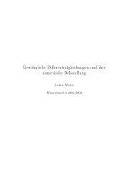
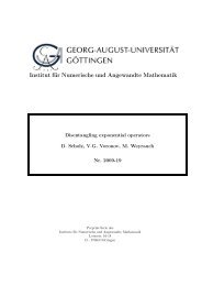
The probability that a customer accepts public transportation
is modeled by the following piecewise linear function (see
left picture of Figure 2):
⎧
⎨
pdij = pd(rij) =
⎩
1
α2−rij
α2−α1
0
:
:
:
rij ≤ α1
α1 < rij ≤ α2
rij > α2
for two parameters α1 and α2.
pw: We determine the average waiting time waitij until the next trip in
Gij starts. To this end, we sort the passengers’ paths in Gij according
to dep(c) to obtain a list dep(c1) < dep(c2) < . . . < dep(cK) with
k ≤ |Gij|. (Note that there are no paths with the same departure
time in Gij.) This yields K − 1 intervals
Ik = [dep(ck), dep(ck+1)], j = k, . . . , K − 1.
7

probability
to accept
1
0
a1 a2 travel time ratio
1.1 2.4 private:public
probability
to accept
1
0
b1
10 min
b2
45 min
waiting time to
next connection
Figure 2: Probability for accepting the average waiting time and the ratio for the
travel time for a path from i to j.
We assume that the demand is distributed evenly within a period,
i.e. at each minute we have the same probability that a person wants
to start his or her journey. If a person arrives within interval Ik, his
minutes. Hence we estimate
or her average waiting time is |Ik−1|
2
wij =
K�
k=1
|Ik|(|Ik| − 1)
2
as the average waiting time for the next trip from i to j. Again,
the probability that a customer accepts the average waiting time is
modeled by a piecewise linear function (see right picture of Figure 2)
⎧
⎪⎨
pwij = pw(wij) =
⎪⎩
β2−wij
β2−β1
depending on the parameters β1 and β2.
1 : wij ≤ β1
: β1 < wij ≤ β2
0 : wij > β2
Assuming that the probability pwij to accept the average waiting time
is independent of the probability pdij to accept the travel time ratio, we
finally get
pij = pwij · pdij
and are hence able to calculate att(U, f, t) according to (2).
Note that the two functions depend on the customers’ behavior which is
represented by the parameters a1, a2, b1, b2 and λ.
In our case study these parameters are set to
• a1 = 1.1, a2 = 2.5 meaning that everybody accepts an increase of
10% of the travel time, but nobody would accept an increase by the
factor 2.5,
8
,
(4)

• b1 = 7.5, b2 = 36, i.e. an average waiting time of 7.5 minutes (referring
to a connection offered four times an hour) is accepted by all
potential passengers, while an average waiting time of more than 36
minutes is not accepted at all. For public transportation at night we
increased these values to 10 and 45.
• Due to Definition 3 of the set of good passengers’ paths, λ has also an
influence on the probability pij. In our case study we chose λ = 1.3.
Note that the specific values for the parameters have been chosen after
discussion with practitioners. They make sense for the local properties of
Göttingen, but need not hold in other environments. For example, in large
cities, we suggest to choose smaller values for b1 and b2.
Our approach can now be summarized:
Phase 1: Design the routes U and the frequencies f of the vehicles.
Phase 2: Split the routes to lines.
Phase 3: Find a timetable t.
The three phases will be described in more detail in Section 5. We remark
that splitting the vehicle routes to lines is just to obtain a nice graphical
representation of the system, but has no influence on its attractiveness or
on its costs (since the lines are not needed to calculate the costs or the
shortest passengers’ paths).
Summarizing, in our problem (P) we are looking for a set of vehicle routes
U, with frequencies fu ∈ IN for each u ∈ U and a timetable tu for each
u ∈ U. A solution is denoted as (U, f, t). Our goal is to find a solution
(U, f, t) with less than N vehicles minimizing att(U, f, t).
3 Complexity
Not very surprisingly, the integrated problem of planning lines, a timetable
and the vehicle schedules is NP hard. More detailed, the following results
hold.
Theorem 3.1.
• It is NP-hard to design the routes of the vehicles, even if the timetable
is not relevant, i.e. Phase 1 of (P) is NP-hard.
• It is NP-hard to find an optimal timetable, even if the vehicle routes
are given, i.e. Phase 3 of (P) is NP-hard.
• The variant (P-special) in which all routes must contain a stop of a
given central location, all frequencies have to be one, the set of edges
with their lengths in the public and in the private mode coincide and
the timetable is not relevant is still NP-hard.
9

We present the proof for the third statement (which also proves the first.)
The proof of the second statement can be found in [Mic07]; intuitively it
also follows from the NP-hardness of periodic scheduling.
More formally, the third problem (P-special) can be described as follows:
(P-special) Given a PTN = (V, E) with edge lengths d(e) = dbus(e) =
dpriv(e) for each e ∈ E, a set of locations B, a central location lc and
an origin-destination matrix OD, values λ, a1, a2, b1, b2 describing the
users’ behavior, a time period T , and two integers N and U, does there
exist a solution (U, f, t) satisfying
• lc ∩ u �= ∅ for all u ∈ U,
• fu = 1 for all u ∈ U,
• �
u∈U
�
e∈U l(e) ≤ N (i.e. it can be run with N busses)
and such that
• �
i=1
�
j=1 pijODij ≥ U ?
Proof. We use a reduction from the knapsack problem which is known
to be NP-hard (see [GJ79]). It is defined as follows: Given two natural
numbers W, B and a set of items D with weights w(d) ∈ IN and benefits
v(d) ∈ IN for all d ∈ D, does there exist a subset K ⊆ D of items with a
total weight of no more than W and a total benefit of at least B?
Given an instance of (Knapsack), an instance of (P-special) is to be constructed.
Define a central location lc and a location ld for each item in
d ∈ D and add exactly one stop sc and sd for all d ∈ D for each of the
locations. Connect all stops sd star-wise to the central stop sc with a pair
of inverse edges. The lengths l(e) of these two edges e ∈ {(sd, sc), (sc, sd)}
is set to w(d)·T
2 for both the public and the private mode for each item
d ∈ D. We furthermore define the demand between the central location
and the locations ld as
ODlc,ld
:= v(d) for each d ∈ D
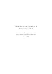
and zero for all other pairs. For an illustration of this instance of (P-special)
see Figure 3.
For the customers’ behavior we set β1 and β2 so large that all waiting times
will be accepted. Furthermore, we set α1 ≥ 1 such that the customers
accept the public mode if the traveling time is the same as in the private
mode. This means that all existing paths are accepted by the passengers,
independently of their timetables. Finally, we define N := W and U := B.
We now show that (P-special) has a feasible solution if and only if (Knapsack)
has a feasible solution.
10

item d
s
d
ud circulation
sc
central
station
Figure 3: Reduction of (P-special) to (Knapsack).
(Knapsack) has a feasible solution: Let a feasible solution for (P-special)
be given with a set U of routes. Every route contains the central
stop lc and at least one other stop. Without loss of generality we
can assume that the route contains exactly one other stop (otherwise
we split it to feasible routes for each other stop sd it contains,
since 2 · dur(e) ≥ T ). We define ud := (sc, sd, sc) as the route passing
through stop sd.
We now show that
K := {d ∈ D : sd ∈ u for some u ∈ U} = {d ∈ D : ud ∈ U}.
is a feasible solution of (Knapsack):
= w(d)T time. Hence, in order to run
this route with a frequency of one, w(d) busses are necessary, see
(1). Since the solution U is feasible for (P-special) we conclude
• The route ud takes 2· w(d)·T
2
that
W ≥
��
u∈U
�
e∈u l(e)
T
�
= �
w(d).
d∈K
• On the other hand, we know that the customers belonging to
location ld will use public transportation whenever sd ∈ u for
some u ∈ U, i.e. whenever ud ∈ U exists. Together with the
feasibility of the solution we obtain
B ≤ �
demand covered by u = �
v(d).
u∈U
(P-special) has a feasible solution: Given a solution K ⊆ D for (Knapsack),
we construct a route ud := (sc, sd, sc) with frequency fd = 1
for each d ∈ K and set U := {ud : d ∈ K}. Then U satisfies the four
conditions listed in the theorem:
11
d∈K

• sc ∈ u for all u ∈ U, hence lc ∩ u �= ∅.
• fu = 1 for all u ∈ U.
• dur(u) = �
u∈U
� �
e∈u l(e) = d∈K
2T w(d)
2
hence
N ≥ number of vehicles = �
� �
dur(u)
=
T
�
w(d)
(i.e. it can be run with N busses)
• U ≤ �
i=1
u∈U
�
j=1 pijODij = �
d∈K v(d)
d∈K
Hence U is feasible for (P-special) and the proof is finished.
4 Case Study
Before outlining our solution approach we describe the data of the case
study we used. The case study was done within a cooperation with Göttinger
Verkehrsbetriebe (GÖVB), the local bus company of Göttingen, Germany.
The data we used consisted of 248 locations with 485 stops. The capacity
of most of the stops is equal to four. It turned out that this is a crucial
constraint: If left out we always obtained timetables in which up to 10
busses stopped simultaneously at the same station. We furthermore indicated
the nodes that are in particular suitable for adding slack times for
breaks.
As edges we used all edges contained in already existing lines, but we also
added further edges representing streets which are currently not used by
busses. The driving times of the new edges were fixed in cooperation with
GÖVB. We also added footpaths between stops.
In order to estimate the traveling time in the private mode, we added
additional edges which are not suitable for busses (e.g. if the streets are
too narrow). The edge lengths in the private mode are usually shorter
then in the public mode. An exception are some streets in the city center
where we added additional time to account for the time-consuming task of
finding a parking slot.
As demand data we received a partition of Göttingen into regions, called
cells and data about the demand for each pair of cells. We assigned locations
to cells (where a location can be assigned to more than one cell, and a
cell can contain more than one location), estimated the importance of each
location and expressed this by weights. Then we distributed the demand
data to pairs of locations according to their assignment and weights.
An analysis of the current system showed its advantages and drawbacks:
The driving times from the outskirts to the center are rather small. Moreover,
twice an hour, many transfers are possible at one of the central stations.
On the other hand, the capacity of this station is exceeded such that
12

usses sometimes have to leave before the transferring passengers have arrived.
We also noted that there are often long breaks at the end-stations
of the lines (up to 20% of the duration of the route).
5 Solution Approach
According to Theorem 3.1, Phase 1 and Phase 3 of our solution approach
are NP-hard by themselves. We therefore suggest to solve both of the
problems heuristically. In the following we present the ideas we used.
Some of them were motivated by the special requirements of Göttingen,
but all of them can easily be adapted to other cities.
Given a solution (U, f, t) we can evaluate its objective value att(U, f, t) as
shown in Section 2. As mentioned on page 9 we proceed in three steps. We
first construct a reasonable set of routes, split them into lines and finally
assign departure and arrival times to them.
Phase 1: Finding the vehicle routes with their frequencies
Each route is a circle in the public transportation network PTN. The basic
idea of the algorithm is simple: We start with an arbitrary station s and
move at random to one of its neighbors. We repeat this procedure until we
end up at the starting station s again. Theoretically we can construct any
route with this procedure, but in practice we have to guide it to obtain
reasonable results. This can be done as follows.
Duration of a route. When generating the routes we keep the restrictions
we have when adding departure and arrival times in mind. There are
several reasons why some breaks (or additional slack time at stations) need
to be added within the trips.
The most important one is to keep periodicity of the schedule. All vehicle
routes should be repeated in each time period. Hence, the time needed for
a route must satisfy
dur(u) · fu = zT
for some integer z. To keep the unused time as small as possible we fix
some (small) ¯η > 0 and only consider routes u with
dur(u) ≤ (z − η) T
where z is an integer and 0 < η < ¯η. It is desirable that η is small,
but not zero such that some additional slack time is available for each
route. Such time can be used to provide slack times at stations in order to
enable passengers to change to other busses, or more general, to make the
13
fu
(5)

timetable robust against delays. It may also be needed for breaks for the
drivers at the end stations. For each route the additional time η has to be
distributed to the edge lengths. We propose to add such time to stopping
times at stations where transfers are likely or to the stations farthest away
from the center at turnaround activities.
In Göttingen, the period T equals 60 minutes. The restriction described
here leads typically to routes with a duration of 60,90, or 120 minutes. The
upper bound for η has been fixed to 10% of T
fu .
Important stations. We identify a set of important locations and
require that each route contains at least one of these stations. This significantly
reduces the search space.
In Göttingen we declared two central locations as important. This means
that all routes pass through the city center. This condition is justified since
the demand between two non-central locations is rather small (according
to the data we had and as expected due to gravity models).
Note that we have seen in part 3 of Theorem 3.1 that the problem remains
NP-complete also with this reduced search space. Without loss of generality
we can start the construction of a route u from such an important
station. Let us call this station su in the following.
Other rules. One can set up many other restrictions or heuristics to
construct and polish the routes found. Some of them are listed below. Let
U be the set of routes already found.
• Stops that have not been covered by any other route of U should be
more likely to be chosen such that we obtain a set of routes covering
all stops. To this end one can weight the neighbors of the current
stop s to increase the probability that a stop is chosen if it still does
not appear in other routes. In our case study, we derived good results
by weighting the unused stops by a factor of three.
• Circles within the routes should be avoided: This can be done by
taking a new stop with a higher probability if it is not already in the
route. (This rule is certainly not applied for the starting node su.)
• It may be desirable that routes contain most of their edges forward
and backward (i.e. have a similar shape in inbound and outbound
direction). To enforce this we suggest to consider only such routes in
which the number of locations that consist of more than one station
but only have one station in the route is small.
• In Göttingen we also implemented the following rule: Let us call a
part of a route starting and ending at an important stop (in the city
center) a branch. The public transportation company in Göttingen
did not want to have routes with four or more branches. We took this
into account by deleting all routes that visited the city center more
than four times. This means that a station from the city center has
14

to appear between 25% and 75% of the (previously fixed) duration of
the route. We used this observation to obtain a further reduction of
the search space.
• Many other rules to model specific requirements are possible.
The algorithm is as follows. In each step we choose a time representing the
duration of a route and a frequency as parameters. Then we construct a set
of lines fitting to these two parameters. We evaluate the routes one by one
and choose the best. The correct evaluation of the attractiveness requires
a timetable which is not at hand during the first phase. Hence we estimate
the objective function by setting all departure times at the (important) stop
from which we started to zero. This ensures that passengers can transfer
without large waiting times at these important stops. Summarizing, we
obtain the following procedure.
Phase 1: Design of routes:
Step 1.1: U = ∅, n = N.
Step 1.2: Fix a frequency fu and dur fix = z·T
fu
cording to (5).
for some integer z ac-
Step 1.3: Design a set of routes u1, . . . uh that include at least one
important station with dur fix − ¯η ≤ dur(uk)x < dur fix for k =
1, . . . , h. One can require that the routes should respect some of
the rules mentioned above.
Step 1.4: Add slack times to the edge lengths of u to obtain a duration
of exactly dur fix .
Step 1.5: Determine ui := maxj=1,...,h att(U ∪ {uj}, f, 0} and add
U := U ∪ {ui}.
Step 1.6: n := n − durfix ·fu
T
Step 1.7: If n > 0 goto Step 2.
Phase 2: Designing the lines
If the vehicle routes have been fixed we can represent them as lines. A line
is a path through the PTN; hence each part of a route can be considered
as a line. As lines are usually organized as tours it is preferable to take
sub-circles of the routes.
As mentioned before, the representation by lines has no effect on where
and when the busses drive and hence no effect on the objective function.
Consequently, we can define the lines such that we get a “nice layout”.
In Göttingen, all routes have to pass through the city center. Moreover,
no route is allowed to contain more than three branches. We hence chose
15

line 5
line 1
center
line 2
line 4
line 3
Figure 4: Three routes that are splitted to five lines.
branches or combinations of pairs of branches as lines, see Figure 4 for an
illustration. These branches naturally are sub-circles of the routes.
Algorithmically, we can proceed as follows.
Phase 2: Splitting routes to lines:
Input: U
Step 2.1: For each route u ∈ U: Decompose U in circles. Choose the
circles or unions of circles as lines.
Phase 3: Finding the timetable
As input for this phase we have given a set of routes U with their frequencies
fu, u ∈ U. Our goal is to construct a feasible timetable. According to
our constraints, a timetable is feasible if there is enough space at each of the
stops in the system. We choose a timetable within the period {0, . . . , T }
which is then repeated periodically. This is taken into account when evaluating
our objective function att.
Since we already added slack time to the edges when constructing the
routes, it is enough to fix one departure time for each route. We take the
stop su from which we started to construct route u. A timetable is hence
given as a vector t ∈ T |U| where T = {0, 1, . . . , T } contains a discrete set
of points in time (usually minutes). We call a timetable t optimal if
att(U, f, t) = max
t ′ ∈T |U|
att(U, f, t ′ ).
16

Consider a route u with frequency fu and departure time tu at stop su.
Then another departures of the same route will take place at tu + z T
fu for
all integer values of z. Hence we only need to evaluate departure times
tu ∈ {0, 1, . . . , T }. Even with this reduction it is not possible to try
fu
all possible combinations of departure times. Since Theorem 3.1 states
that the problem of finding an optimal timetable is NP-hard we propose
to use a heuristic also in this phase. The first idea to fix the departure
times of each routes iteratively had the following drawback: We obtained
routes, all departing at the same time from the same central station. When
the capacity of this station was used, the next routes were placed very
disadvantageous such that the final outcome was not really good.
We hence developed the following approach. We divide the routes into pairs
and synchronize each pair in a first step. In a second step we combine the
pairs to quadruples and synchronize them. We proceed in this manner until
all routes are fixed. During this process we choose the pairs in each step
by matching techniques to ensure that the most promising combinations
are grouped.
More precisely, we define the following graph Gmatch = (U, Ematch) in
which the nodes are defined as the routes U and we add an edge between
two routes u1, u2 if u1 ∩ u2 �= ∅, i.e. if they contain at least one stop where
a transfer is possible. As weight for edge {u1, u2} we set
cu1,u2
:= max
t1,t2∈T att({u1, u2}, {fu1 , fu2 }, (t1, t2)),
i.e. we choose the best possible synchronization of the two routes (independent
of all other lines). Since one of the two times t1, t2 can arbitrarily
be fixed we only have to evaluate
cu1,u2
:= max
t∈T att({u1, u2}, {fu1 , fu2 }, (0, t)) (6)
We then choose a cost-maximal matching in the graph Gmatch which synchronizes
pairs of routes. Each of the pairs (or of single routes if the
matching was not a perfect matching) is then clustered to one new node
for the matching graph of the next step. In the second step we find an
optimal matching of the groups and go on until only one group is left.
To state the algorithm we need to deal with groups of routes g ⊂ U.
Synchronizing such a group of routes means to find a timetable
tg := (tu : u ∈ g)
for all routes u ∈ g. Note that such a timetable can be shifted in time
without changing its objective value, i.e.
att(g, fu : u ∈ g, tg) = att(g, fu : u ∈ g, tg + t)
17

where tg + t = (tu + t : u ∈ g). We can hence assume without loss of
generality that there is one representative route ug in each group g with
tug = 0.
Given two two groups of routes g1 and g2 with two timetables tg1
and tg2 .
If we want to synchronize these groups (without changing their internal
timetables) we have to find
max
t∈T att(g1 ∪ g2, (fu, u ∈ g1 ∪ g2), (tg1 , t + tg2 ))
The optimal value for t is denoted as t ∗ g1,g2
shift.
and called the synchronization
Our algorithm starts with a first partition into groups, each group consisting
of only one route. In each step, the groups are matched pairwise.
(Some groups may be left unmatched if the matching is not perfect, but
since the matching graph is nearly complete this is usually at most one
group.)
The procedure can be summarized as follows.
18

Phase 3: Finding the timetable
Input: U, fu for all u ∈ U.
Step 3.1: Define the first matching graph Gmatch = (Vmatch, Ematch)
with
• Vmatch = {{u} : u ∈ U}
• ug = u if g = {u} as representative route of group g
• tg = (0) as timetable of group g
• Ematch := {{g1, g2} : there exists u1 ∈ g1, u2 ∈
g2 such that u1 ∩ u2 �= ∅}
• cg1,g2 := maxt∈T att(g1 ∪ g2, (fu, u ∈ g1 ∪ g2), (tg1 , t + tg2 )) and
be the corresponding synchronization shift.
let t ∗ g1,g2
Step 3.2: Find a matching E m ⊆ Ematch maximizing the sum of
weights.
Step 3.3: Update groups: For each e = {g1, g2} ∈ E m define g :=
g1 ∪ g2 and
• Vmatch = Vmatch ∪ {g} \ {g1, g2}
• ug = ug1 as representative route of group g
• tg = (tg1 , t∗g1,g2 + tg2 ) as timetable of group g using the synchronization
shift calculated before.
Step 3.4: Update matching graph:
• Ematch := {{g1, g2} : there exists u1 ∈ g1, u2 ∈
g2 such that u1 ∩ u2 �= ∅}
• cg1,g2 := maxt∈T att(g1 ∪ g2, (fu, u ∈ g1 ∪ g2), (tg1 , t + tg2 )) and
be the corresponding synchronization shift.
let t ∗ g1,g2
Step 3.5: If Ematch = ∅ stop. Output: (tg : g ∈ Vmatch).
Otherwise goto Step 3.2.
After fixing a timetable with the above algorithm we used an improvement
heuristic checking the distribution of the slack times which appear in equation
(5) and have already been fixed in Phase 1. A redistribution may lead
to further possibilities to transfer and hence further improve the objective
function.
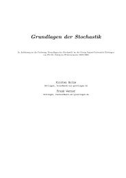
6 Results and Conclusion
We implemented our procedures and tested them within a case study in
Göttingen. Our program needed 20 hours to generate a solution with 8
routes which we splitted to 10 lines. The solution improves the attractiveness
of the current solution by 18.7%. The new timetable does not have
19

Figure 5: Comparison of new and old lines in Göttingen.
System at night: System at daytime:
current system. 23 busses, 11 routes 46 busses, 13 routes
“best” system 23 busses, 8 routes 42 busses, 12 routes
improvement costs by 0%, att by 18% costs by 10%, att by 1%
Table 1: The best solutions of our algorithm.
the long breaks at the ends of the lines and uses the additional busses to
increase the frequencies of the routes. Moreover it is more robust due to
the distribution of the slack times and it takes the capacities of the stations
into account. The current lines and the new lines are shown in Figure 5.
The figure shows that (nearly) all edges that have been covered by a route
before are still covered. But the shape of the single vehicle routes changed,
and also their durations and frequencies.
By decreasing the number of available busses we can also use the program
to optimize the costs instead of the attractiveness of the system. This
yielded a reduction of 10% of the busses and still increased the attractiveness
by 1%. The two solutions which are best according to the practitioners
of GÖVB are listed in Table 6.
At the moment, GÖVB is implementing the results in its new line system.
Summarizing, we presented a new integrated approach to tackle three
problems in public transportation: line planning, timetabling and vehicle
scheduling. We did not use the classical sequence of the planning phases
but started by constructing the vehicle routes. Both phases, constructing
the routes and fixing the timetable are NP-hard. In this paper we suggested
heuristic solutions which worked very well in practice. However,
we are sure that improvements can be made in both procedures and more
theoretical results about these new types of problems can be obtained.
20

References
[ARR] ARRIVAL. Future and Emerging Technologies Unit of EC
(IST priority - 6th FP), under contract no. FP6-021235-2. see
http://arrival.cti.gr.
[BCG87] A. Bertosi, P. Carrarresi, and G. Gallo. On some matching
problems arising in vehicle scheduling models. Networks,
17:271–281, 1987.
[BDW07] Reinhard Bauer, Daniel Delling, and Dorothea Wagner. Experimental
Study on Speed-Up Techniques for Timetable Information
Systems. In Proceedings of the 7th Workshop on Algorithmic
Approaches for Transportation Modeling, Optimization,
and Systems (ATMOS’07). Schloss Dagstuhl, Germany,
2007.
[BGP05] R. Borndörfer, M. Grötschel, and M. E. Pfetsch. A path-based
model for line planning in public transport. Technical Report
05-18, ZIP Berlin, 2005.
[BK06] S. Bunte and N. Kliewer. An overview on vehcile scheduling
models. In proceedings of Computer-Aided Scheduling of Public
Transport (CASPT). 2006.
[BKZ96] M.R. Bussieck, P. Kreuzer, and U.T. Zimmermann. Optimal
lines for railway systems. European Journal of Operational Research,
96(1):54–63, 1996.
[BLL04] M.R. Bussieck, T. Lindner, and M.E. Lübbecke. A fast algorithm
for near cost optimal line plans. Mathematical Methods
of Operational Research, 59(3):205–220, 2004.
[BP05] R. Borndörfer and M. E. Pfetsch. Routing in line planning
for public transportation. Technical Report 05-36, ZIP Berlin,
2005.
[Bus98] M.R. Bussieck. Optimal lines in public transport. PhD thesis,
Technische Universität Braunschweig, 1998.
[CvDZ98] M.T. Claessens, N.M. van Dijk, and P.J. Zwaneveld. Cost optimal
allocation of rail passenger lines. European Journal on
Operational Research, 110:474–489, 1998.
[DP95] J. R. Daduna and J. M. P. Paixao. Vehicle scheduling for
public mass transit – an overview. In Computer-Aided Transit
Scheduling, number 430 in Lecture Notes in Economics and
Mathematical Systems, pages 76–90. Springer, 1995.
[FSZ07] M. Fischetti, D. Salvagnin, and A. Zanette. Fast
approaches to robust railway timetabling. Technical
Report TR-0094, ARRIVAL Report, 2007.
http://arrival.cti.gr/index.php/Documents/Main.
21

[GJ79] M.R. Garey and D.S. Johnson. Computers and Intractability
— A Guide to the Theory of NP-Completeness. Freeman, San
Francisco, 1979.
[Goo04] J. Goossens. Models and algorithms for railway line planning
problems. PhD thesis, University of Maastricht, 2004.
[GS78] B. Gavish and E. Shlifer. An approach for solving a class for
transportation scheduling problems. European Journal of Operational
Research, 3:122–134, 1978.
[GvHK06] J. Goossens, C.P.M. van Hoesel, and L.G. Kroon. On solving
multi-type railway line planning problems. European Journal
of Operational Research, 168(2):403–424, 2006.
[KDV07] L.G. Kroon, R. Dekker, and M. Vromans. Cyclic railway
timetabling: A stochastic optimization approach. In Algorithmic
Methods for Railway Optimization, number 4359 in Lecture
Notes in Computer Science. Springer, 2007.
[KGS06] N. Kliewer, V. Gintner, and L. Suhl. Line change considerations
within a time-space network based multi-depot bus scheduling
model. In proceedings ov CASPT IX, 2006.
[Lie06] C. Liebchen. Periodic Timetable Optimization in Public Transport.
dissertation.de – Verlag im Internet, Berlin, 2006.
[LM04] C. Liebchen and R. Möhring. The modeling power of the periodic
event scheduling problem: Railway timetables - and
beyond. In Proceedings of 9th meeting on Computer-Aided
Scheduling of Public Transport(CASPT 2004). 2004.
[LM06] C. Liebchen and R. Möhring. The modeling power of the periodic
event scheduling problem: railway timetables — and beyond.
In Algorithmic Methods for Railway Optimization, Lecture
Notes on Computer Science. Springer, 2006.
[LMO05] G. Laporte, J.A. Mesa, and F.A. Ortega. Maximizing trip
coverage in the location of a single rapid transit alignment.
Annals of Operations Research, 136:49–63, 2005.
[LnMO06] G. Laporte, A. Marín, J.A. Mesa, and F.A. Ortega. An integrated
methodology for rapid transit network design. In Algorithmic
Methods for Railway Optimization, Lecture Notes on
Computer Science. Springer, 2006. Presented at ATMOS 2004.
[LSS + 07] C. Liebchen, M. Schachtebeck, A. Schöbel, S. Stiller, and
A. Prigge. Computing delay-resistant railway timetables.
Technical Report TR-0066, ARRIVAL Report, 2007. see
http://arrival.cti.gr/index.php/Documents/Main.
[Löb97] A. Löbel. Optimal vehicle scheduling in public transit. PhD
thesis, Technische Universität Berlin, 1997.
22

[Mar06] G. Maróti. Operations Research Models for Railway Rolling
Stock Planning. PhD thesis, Eindhoven University of Technology,
Eindhoven, The Netherlands, 2006.
[Mic07] M. Michaelis. Integrierte Linien- und Umlaufplanung sowie
Fahrplangenerierung für den ÖPNV. Master’s thesis, Georg-
August Universität Göttingen, 2007. in German.
[Nac94] K. Nachtigall. A branch and cut approach for periodic network
programming. Technical Report 29/94, Hildesheimer
Informatik-Berichte, 1994.
[Orl76] C.S. Orloff. Route constraint fleet scheduling. Transportation
Science, 10(2):149–168, 1976.
[Pat25] A. Patz. Die richtige auswahl von verkehrslinien bei großen
strassenbahnnetzen. Verkehrstechnik, 50/51, 1925.
[PDHH06] A.-S. Pepin, G. Desaulniers, A. Hertz, and D. Huisman. Comparison
of heuristic approaches for the multiple depot vehicle
scheduling problem. Technical Report TR-0044, ARRIVAL Report,
2006. http://arrival.cti.gr/index.php/Documents/Main.
[Pee02] L. Peeters. Cyclic Railway Timetabling Optimization. PhD
thesis, ERIM, Rotterdam School of Management, 2002.
[Qua03] C. B. Quak. Bus line planning. Master’s thesis, TU Delft, 2003.
[Sah72] J.L. Saha. An algorithm for bus scheduling problems. Operational
Research Quaterly, 21(4):463–474, 1972.
[Sch05] S. Scholl. Customer-oriented line planning. PhD thesis, Technische
Universität Kaiserslautern, 2005.
[Son77] H. Sonntag. Linienplanung im öffentlichen Personennahverkehr.
PhD thesis, TU Berlin, 1977.
[SS06] A. Schöbel and S. Scholl. Line planning with minimal transfers.
In 5th Workshop on Algorithmic Methods and Models for
Optimization of Railways, number 06901 in Dagstuhl Seminar
Proceedings, 2006.
[SU89] P. Serafini and W. Ukovich. A mathematical model for periodic
scheduling problems. SIAM Journal on Discrete Mathematic,
2:550–581, 1989.
[UP95] E. Reinecke U. Pape, Y.-S. Reinecke. Line network planning. In
Computer-Aided Scheduling of Public Transport, number 430 in
Lecture Notes in Economics and Mathematical Systems, 1995.
[Zwa97] P.J. Zwaneveld. Railway Planning — Routing of trains and allocation
of passenger lines. PhD thesis, School of Management,
Rotterdam, 1997.
23

Institut für Numerische und Angewandte Mathematik
Universität Göttingen
Lotzestr. 16-18
D - 37083 Göttingen
Telefon: 0551/394512
Telefax: 0551/393944
Email: trapp@math.uni-goettingen.de URL: http://www.num.math.uni-goettingen.de
Verzeichnis der erschienenen Preprints 2008:
2008-01 M. Körner, A. Schöbel Weber problems with high-speed curves
2008-02 S. Müller, R. Schaback A Newton Basis for Kernel Spaces
2008-03 H. Eckel, R. Kress Nonlinear integral equations for the complete
electrode model in inverse impedance
tomography
2008-04 M. Michaelis, A. Schöbel Integrating Line Planning, Timetabling, and Vehicle
Scheduling: A customer-oriented approach