JMP INTRO ® Lab Activities Lab Activity – Hypothesis Testing – the t ...

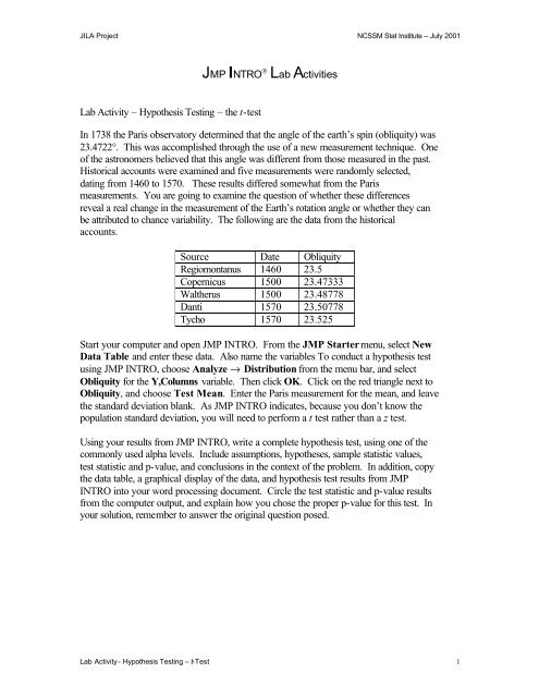
JILA Project NCSSM Stat Institute – July 2001JMP INTRO ® Lab ActivitiesLab Activity – Hypothesis Testing – the t-testIn 1738 the Paris observatory determined that the angle of the earth’s spin (obliquity) was23.4722°. This was accomplished through the use of a new measurement technique. Oneof the astronomers believed that this angle was different from those measured in the past.Historical accounts were examined and five measurements were randomly selected,dating from 1460 to 1570. These results differed somewhat from the Parismeasurements. You are going to examine the question of whether these differencesreveal a real change in the measurement of the Earth’s rotation angle or whether they canbe attributed to chance variability. The following are the data from the historicalaccounts.Source Date ObliquityRegiomontanus 1460 23.5Copernicus 1500 23.47333Waltherus 1500 23.48778Danti 1570 23.50778Tycho 1570 23.525Start your computer and open JMP INTRO. From the JMP Starter menu, select NewData Table and enter these data. Also name the variables To conduct a hypothesis testusing JMP INTRO, choose Analyze fi Distribution from the menu bar, and selectObliquity for the Y,Columns variable. Then click OK. Click on the red triangle next toObliquity, and choose Test Mean. Enter the Paris measurement for the mean, and leavethe standard deviation blank. As JMP INTRO indicates, because you don’t know thepopulation standard deviation, you will need to perform a t test rather than a z test.Using your results from JMP INTRO, write a complete hypothesis test, using one of thecommonly used alpha levels. Include assumptions, hypotheses, sample statistic values,test statistic and p-value, and conclusions in the context of the problem. In addition, copythe data table, a graphical display of the data, and hypothesis test results from JMPINTRO into your word processing document. Circle the test statistic and p-value resultsfrom the computer output, and explain how you chose the proper p-value for this test. Inyour solution, remember to answer the original question posed.Lab Activity - Hypothesis Testing – t-Test 1

JILA Project NCSSM Stat Institute – July 2001JMP INTRO ® Lab ActivitiesTeacher NotesLab Activity – Hypothesis Testing – the t-testObjectives:• Gain familiarity with some of the basic operational tools of JMP INTRO.• Use JMP INTRO to conduct a hypothesis test for a mean when the standarddeviation is unknown.• Create a word processing document, incorporating displays from JMP INTRO.Time Required:Materials:30 minutesHypothesis Testing - the t-test student activity directionsPrerequisites:• Students should have basic knowledge of how to use JMP INTRO.• Students should have experience conducting tests of hypothesis by hand and/orwith graphing calculators for a mean when the standard deviation is unknown.• Students should have experience writing conclusions in the context of theproblem for hypothesis tests.• Students should have had experience creating a data table in JMP INTRO.JMP INTRO Notes:• JMP INTRO includes an extensive online help system. It contains a table ofcontents and/or can be used to search for a specific topic. In addition, JMPINTRO has context sensitive help. You can access it by selecting the help tool (?)from the tools toolbar and clicking inside a data table or report. JMP INTROopens help specific to the clicked-on item.• Students need to choose the correct p-value based on their alternate hypothesis. Abrief discussion of the three p-values reported by JMP INTRO may be necessary.• The Normal Quantile Plot option adds a graph to the report that is useful forvisualizing the extent to which the variable is normally distributed. If a variable isnormal, the normal quantile plot approximates a diagonal straight line. This kindof plot is also called a quantile-quantile plot, or Q-Q plot.Lab Activity - Hypothesis Testing – t-Test 2

JILA Project NCSSM Stat Institute – July 2001JMP INTRO ® Lab ActivitiesAnswer KeyThe following are suggested answers for Hypothesis Testing – the t-test.Assumptions:We were told the data came from a random sample of historicalaccounts. Although there were only five data values, examiningthe plots of the data, along with the normal quantile plot, we haveno reason to believe the data are not normally distributed.Hypotheses: H o : µ = 23.4722 The average Earth obliquity angle was23.4722 degrees in the 15 th and 16 th century.H a : µ ≠ 23.4722 The average Earth obliquity angle was not23.4722 degrees.Test Mechanics:Conclusions:Data:x −µ23.498778−23.4722t = = = 3.0301s 0.019613n5p = 0.0388At the α = .05 level, because p = 0.0388 < 0.05, we should rejectthe null hypothesis and accept the alternative hypothesis. We haveevidence to show the average obliquity was not 23.4722 degreesand have evidence to show that these differences reveal a changein the Earth’s rotation angle.Source Date ObliquityRegiomontanus 1460 23.5Copernicus 1500 23.47333Waltherus 1500 23.48778Danti 1570 23.50778Tycho 1570 23.525Lab Activity - Hypothesis Testing – t-Test 3

JILA Project NCSSM Stat Institute – July 2001Graphical Display:.99.95.90.75.503210Normal Quantile Plot.25.10.05.01-1-223.47 23.48 23.49 23.5 23.51 23.52 23.53JMP INTRO Hypothesis Test Results:Test Mean=valueHypothesized Value 23.4722Actual Estimate 23.4988df 4Std Dev 0.01961t TestTest Statistic 3.0301Prob > |t| 0.0388Prob > t 0.0194Prob < t 0.9806The p-value of 0.0388 was chosen because this was a two-sided test.Lab Activity - Hypothesis Testing – t-Test 4