Dynamical Systems in Neuroscience:

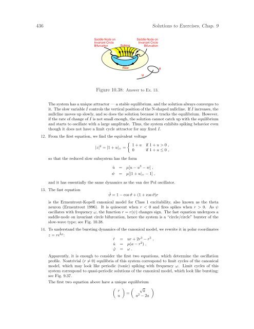
436 Solutions to Exercises, Chap. 9Saddle-Node onInvariant CircleBifurcationSpikingSaddle-Node onInvariant CircleBifurcationRestψθFigure 10.38: Answer to Ex. 13.The system has a unique attractor — a stable equilibrium, and the solution always converges toit. The slow variable I controls the vertical position of the N-shaped nullcline. If I increases, thenullcline moves up slowly, and so does the solution because it tracks the equilibrium. However,if the rate of change of I is not small enough, the solution cannot catch up with the equilibriumand starts to oscillate with a large amplitude. Thus, the system exhibits spiking behavior eventhough it does not have a limit cycle attractor for any fixed I.12. From the first equation, we find the equivalent voltage{|z| 2 1 + u if 1 + u > 0 ,= |1 + u| + =0 if 1 + u ≤ 0 ,so that the reduced slow subsystem has the form˙u = µ[u − u 3 − w] ,ẇ = µ[|1 + u| + − 1] ,and it has essentially the same dynamics as the van der Pol oscillator.13. The fast equation˙ϑ = 1 − cos ϑ + (1 + cos ϑ)ris the Ermentrout-Kopell canonical model for Class 1 excitability, also known as the thetaneuron (Ermentrout 1996). It is quiescent when r < 0 and fires spikes when r > 0. As ψoscillates with frequency ω, the function r = r(ψ) changes sign. The fast equation undergoes asaddle-node on invariant circle bifurcation, hence the system is a “circle/circle” burster of theslow-wave type; see Fig. 10.38.14. To understand the bursting dynamics of the canonical model, we rewrite it in polar coordinatesz = re iϕ :ṙ = ur + 2r 3 − r 5 ,˙u = µ(a − r 2 ) ,˙ϕ = ω .Apparently, it is enough to consider the first two equations, which determine the oscillationprofile. Nontrivial (r ≠ 0) equilibria of this system correspond to limit cycles of the canonicalmodel, which may look like periodic (tonic) spiking with frequency ω. Limit cycles of thissystem correspond to quasi-periodic solutions of the canonical model, which look like bursting;see Fig. 9.37.The first two equation above have a unique equilibrium( ) ( √ )r a=u a 2 − 2a