Dynamical Systems in Neuroscience:

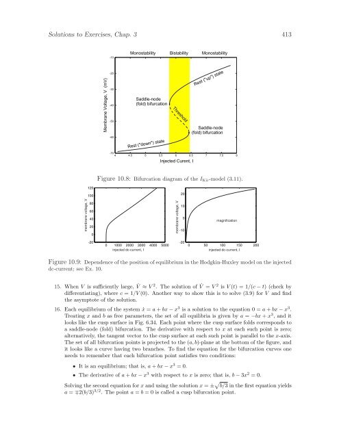
Solutions to Exercises, Chap. 3 413-10MonostabilityBistabilityMonostabilityMembrane Voltage, V (mV)-20-30-40-50-60Saddle-node(fold) bifurcationRest ("down") stateThreshold-704 4.5 5 5.5 6 6.5 7 7.5 8Injected Curent, IRest ("up") stateSaddle-node(fold) bifurcationFigure 10.8: Bifurcation diagram of the I Kir -model (3.11).12010020membrane voltage, V806040200membrane voltage, V100-10magnification-200 1000 2000 3000 4000 5000injected dc-current, I-200 50 100 150 200injected dc-current, IFigure 10.9: Dependence of the position of equilibrium in the Hodgkin-Huxley model on the injecteddc-current; see Ex. 10.15. When V is sufficiently large, ˙V ≈ V 2 . The solution of ˙V = V 2 is V (t) = 1/(c − t) (check bydifferentiating), where c = 1/V (0). Another way to show this is to solve (3.9) for V and findthe asymptote of the solution.16. Each equilibrium of the system ẋ = a + bx − x 3 is a solution to the equation 0 = a + bx − x 3 .Treating x and b as free parameters, the set of all equilibria is given by a = −bx + x 3 , and itlooks like the cusp surface in Fig. 6.34. Each point where the cusp surface folds corresponds toa saddle-node (fold) bifurcation. The derivative with respect to x at each such point is zero;alternatively, the tangent vector to the cusp surface at each such point is parallel to the x-axis.The set of all bifurcation points is projected to the (a, b)-plane at the bottom of the figure, andit looks like a curve having two branches. To find the equation for the bifurcation curves oneneeds to remember that each bifurcation point satisfies two conditions:• It is an equilibrium; that is, a + bx − x 3 = 0.• The derivative of a + bx − x 3 with respect to x is zero; that is, b − 3x 2 = 0.Solving the second equation for x and using the solution x = ± √ b/3 in the first equation yieldsa = ∓2(b/3) 3/2 . The point a = b = 0 is called a cusp bifurcation point.