- Page 1:
Eugene M. IzhikevichThe Neuroscienc
- Page 6 and 7:
6.3.6 Saddle-node homoclinic orbit
- Page 8 and 9:
9.4.2 Integrators vs. Resonators .
- Page 10 and 11:
xPrefaceversely, cells having quite
- Page 12 and 13:
2 Introductionapical dendritessomar
- Page 14 and 15:
4 Introduction(a)spikes(b)spikes cu
- Page 16 and 17:
6 Introduction1.1.3 Why are neurons
- Page 18 and 19:
8 Introductionconcepts of dynamical
- Page 20 and 21:
10 Introductionspikingmoderesting m
- Page 22 and 23:
12 Introduction(a)spikinglimitcycle
- Page 24 and 25:
14 Introductionco-existence of rest
- Page 26 and 27:
16 Introduction1.2.4 Neuro-computat
- Page 28 and 29:
18 IntroductionspikeFigure 1.16: Ph
- Page 30 and 31:
20 Introductionwith coupled neurons
- Page 32 and 33:
22 IntroductionFigure 1.17: John Ri
- Page 34 and 35:
24 Introduction
- Page 36 and 37:
26 Electrophysiology of NeuronsInsi
- Page 38 and 39:
28 Electrophysiology of Neuronsouts
- Page 40 and 41:
30 Electrophysiology of NeuronsRest
- Page 42 and 43:
32 Electrophysiology of NeuronsFigu
- Page 44 and 45:
34 Electrophysiology of Neuronsm (V
- Page 46 and 47:
36 Electrophysiology of Neurons10.8
- Page 48 and 49:
38 Electrophysiology of Neurons2.3
- Page 50 and 51:
40 Electrophysiology of NeuronsFigu
- Page 52 and 53:
42 Electrophysiology of NeuronsDepo
- Page 54 and 55:
44 Electrophysiology of NeuronsV(x,
- Page 56 and 57:
46 Electrophysiology of Neurons1m (
- Page 58 and 59:
48 Electrophysiology of NeuronsPara
- Page 60 and 61:
50 Electrophysiology of NeuronsFigu
- Page 62 and 63:
52 Electrophysiology of Neuronsvolt
- Page 64 and 65:
54 Electrophysiology of Neurons
- Page 66 and 67:
56 One-Dimensional SystemsActivatio
- Page 68 and 69:
58 One-Dimensional Systemsinwardcur
- Page 70 and 71:
60 One-Dimensional Systems40bistabi
- Page 72 and 73:
62 One-Dimensional Systemsat every
- Page 74 and 75:
64 One-Dimensional Systems?F(V)>0+
- Page 76 and 77:
66 One-Dimensional SystemsUnstableE
- Page 78 and 79:
¡ ¡ ¡¡ ¡ ¡¡ ¡ ¡¡ ¡ ¡¡
- Page 80 and 81:
70 One-Dimensional Systems+ - - + +
- Page 82 and 83:
72 One-Dimensional Systemsλ(V-Veq)
- Page 84 and 85:
74 One-Dimensional Systemsbifurcati
- Page 86 and 87:
76 One-Dimensional Systems100806040
- Page 88 and 89:
78 One-Dimensional Systemsbifurcati
- Page 90 and 91:
80 One-Dimensional Systems20 mV100
- Page 92 and 93:
82 One-Dimensional Systemsmembrane
- Page 94 and 95:
84 One-Dimensional Systemssteady-st
- Page 96 and 97:
86 One-Dimensional Systemsspike rig
- Page 98 and 99:
88 One-Dimensional SystemsVF (V)1VV
- Page 100 and 101:
90 One-Dimensional Systems10.80.60.
- Page 102 and 103:
92 One-Dimensional Systems
- Page 104 and 105:
94 Two-Dimensional SystemsI Na,pneu
- Page 106 and 107:
96 Two-Dimensional Systemsdefines a
- Page 108 and 109:
98 Two-Dimensional Systems(f(x(t),y
- Page 110 and 111:
100 Two-Dimensional Systems0.70acti
- Page 112 and 113:
102 Two-Dimensional Systems0.70.6K
- Page 114 and 115:
104 Two-Dimensional Systemsy1.510.5
- Page 116 and 117:
106 Two-Dimensional SystemsFor exam
- Page 118 and 119:
108 Two-Dimensional SystemsIn gener
- Page 120 and 121:
110 Two-Dimensional Systemsv 2 v 2v
- Page 122 and 123:
112 Two-Dimensional SystemsV-nullcl
- Page 124 and 125:
114 Two-Dimensional SystemsV-nullcl
- Page 126 and 127:
116 Two-Dimensional Systemsheterocl
- Page 128 and 129:
118 Two-Dimensional Systems0.60.5n-
- Page 130 and 131:
120 Two-Dimensional Systemseigenval
- Page 132 and 133:
122 Two-Dimensional SystemsK + acti
- Page 134 and 135:
124 Two-Dimensional Systemsexcitati
- Page 136 and 137:
126 Two-Dimensional SystemsReview o
- Page 138 and 139:
128 Two-Dimensional SystemsabcdFigu
- Page 140 and 141:
130 Two-Dimensional SystemsFigure 4
- Page 142 and 143:
132 Two-Dimensional Systems
- Page 144 and 145:
134 Conductance-Based Models• If
- Page 146 and 147:
136 Conductance-Based Modelsinward(
- Page 148 and 149:
138 Conductance-Based Models1I=01I=
- Page 150 and 151:
140 Conductance-Based Modelsleak cu
- Page 152 and 153:
142 Conductance-Based Modelshyperpo
- Page 154 and 155:
144 Conductance-Based Models0I=0ina
- Page 156 and 157:
146 Conductance-Based Models0I=9.75
- Page 158 and 159:
148 Conductance-Based Models1I=651I
- Page 160 and 161:
150 Conductance-Based Modelshave co
- Page 162 and 163:
152 Conductance-Based Models1 sec10
- Page 164 and 165:
154 Conductance-Based Modelsvoltage
- Page 166 and 167:
156 Conductance-Based Models1h=0.89
- Page 168 and 169:
158 Conductance-Based Models5.2.2 E
- Page 170 and 171:
160 Conductance-Based Models1recove
- Page 172 and 173:
162 Conductance-Based Modelscurrent
- Page 174 and 175:
164 Conductance-Based Modelsmodels
- Page 176 and 177:
166 Conductance-Based Models
- Page 178 and 179:
168 Bifurcationssaddle-node bifurca
- Page 180 and 181:
170 Bifurcationssaddle-node bifurca
- Page 182 and 183:
172 Bifurcations0.5v 2V-nullclineK
- Page 184 and 185:
174 BifurcationsBoth types of the b
- Page 186 and 187:
176 BifurcationsV-nullcline0.5K + g
- Page 188 and 189:
178 Bifurcationsrstable limit cycle
- Page 190 and 191:
180 BifurcationsnVstable limit cycl
- Page 192 and 193:
¡ ¡¡ ¡¡ ¡ ¡¡ ¡ ¡182 Bifur
- Page 194 and 195:
¡ ¡ ¡¡ ¡ ¡¡ ¡ ¡¡ ¡ ¡184
- Page 196 and 197:
186 Bifurcationsmembrane potential,
- Page 198 and 199:
188 BifurcationsBifurcation of a li
- Page 200 and 201:
190 Bifurcationsstableunstablelimit
- Page 202 and 203:
192 Bifurcationsamplitude (max-min)
- Page 204 and 205:
194 Bifurcationshomoclinic orbithom
- Page 206 and 207:
196 Bifurcations0.80.60.4stable lim
- Page 208 and 209:
198 Bifurcationsfrequency (Hz)40030
- Page 210 and 211:
200 BifurcationsSaddle-Focus Homocl
- Page 212 and 213:
202 Bifurcationsc 1c 2xFigure 6.34:
- Page 214 and 215:
204 BifurcationseigenvaluesHopffold
- Page 216 and 217:
206 Bifurcationsfast nullclineslow
- Page 218 and 219:
208 Bifurcationswith fast and slow
- Page 220 and 221:
210 BifurcationsSupercritical Andro
- Page 222 and 223:
212 BifurcationsK + conductance tim
- Page 224 and 225:
214 BifurcationsIn contrast, if the
- Page 226 and 227:
216 Bifurcationsinvariant circlesad
- Page 228 and 229:
218 Bifurcationsbifurcationssaddle-
- Page 230 and 231:
220 BifurcationsExercises1. (Transc
- Page 232 and 233:
222 Bifurcationsv 2v 11a-11-1Figure
- Page 234 and 235:
224 Bifurcations19. [M.S.] A leaky
- Page 236 and 237:
226 Excitabilityspike?spikerestrest
- Page 238 and 239:
228 ExcitabilityAlternatively, the
- Page 240 and 241:
230 Excitability50 ms 20 mV 1 ms100
- Page 242 and 243:
232 ExcitabilityClass 3 excitable n
- Page 244 and 245:
234 Excitability0.20.150.10.05I 1I
- Page 246 and 247:
236 Excitabilitysaddle-node bifurca
- Page 248 and 249:
238 Excitability(a) resting spiking
- Page 250 and 251:
240 Excitabilityproperties integrat
- Page 252 and 253:
242 ExcitabilityThe existence of fa
- Page 254 and 255:
244 Excitability1coincidencedetecti
- Page 256 and 257:
246 Excitabilityspikeexcitatory pul
- Page 258 and 259:
248 Excitability(g)9 ms(f)(e)(d)(c)
- Page 260 and 261:
250 Excitabilitysquid axonmodel0 mV
- Page 262 and 263:
252 Excitability(a) integrator(b) r
- Page 264 and 265:
254 Excitability(a) integrator(b) r
- Page 266 and 267:
256 Excitabilitymembrane potential,
- Page 268 and 269:
258 Excitability0.1saddle-node bifu
- Page 270 and 271:
260 Excitability100 ms10 mVoscillat
- Page 272 and 273:
262 ExcitabilityBogdanov-Takens bif
- Page 274 and 275:
264 Excitabilitya pulse of current.
- Page 276 and 277:
266 Excitabilitymembrane potential
- Page 278 and 279:
268 Excitability(a)150100I K(M)(b)3
- Page 280 and 281:
270 Excitability50 mV300 msFigure 7
- Page 282 and 283:
272 Excitability20 mVADP100 msAHP-6
- Page 284 and 285:
274 ExcitabilityK + activation gate
- Page 286 and 287:
276 ExcitabilityBibliographical Not
- Page 288 and 289:
278 Excitability7. Show that the re
- Page 290 and 291:
280 Simple Modelsspikemembrane pote
- Page 292 and 293:
282 Simple Models1thresholdyz reset
- Page 294 and 295:
284 Simple Models1v reset =|b| 1/2b
- Page 296 and 297:
286 Simple Modelsbe an integrator o
- Page 298 and 299:
288 Simple Modelsintegrate-and-fire
- Page 300 and 301:
290 Simple Models(A) tonic spiking(
- Page 302 and 303:
292 Simple Modelsgeneral algorithm
- Page 304 and 305:
294 Simple Modelscha, cha — real
- Page 306 and 307:
296 Simple Modelslayer 5 neuronsimp
- Page 308 and 309:
298 Simple Modelsb=-240200saddle-no
- Page 310 and 311:
300 Simple Models(a)simple modellay
- Page 312 and 313:
302 Simple Models(a)burstingspiking
- Page 314 and 315:
304 Simple Models(a)dendriticspike2
- Page 316 and 317:
306 Simple Models(a)74 5 6 3210(b)C
- Page 318 and 319:
308 Simple Modelschattering neuron
- Page 320 and 321:
310 Simple ModelsLTS neuron (in vit
- Page 322 and 323:
312 Simple ModelsFS neuron (in vitr
- Page 324 and 325:
314 Simple Models(1) fast oscillati
- Page 326 and 327:
316 Simple Modelsthrough an appropr
- Page 328 and 329:
318 Simple Modelsthey are able to g
- Page 330 and 331:
320 Simple Modelsv r = −80 mV, an
- Page 332 and 333:
322 Simple Modelsshow in Fig. 7.36.
- Page 334 and 335:
324 Simple ModelsBibliographical No
- Page 336 and 337:
326 Simple ModelsExercises1. (Integ
- Page 338 and 339:
328 Simple Models17. [M.S.] Analyze
- Page 340 and 341:
330 Simple Modelsa35 mV350 msc-NAC
- Page 342 and 343:
332 Simple Modelsrat RTN neuronsimp
- Page 344 and 345:
334 Simple ModelsFigure 8.34: Class
- Page 346 and 347:
336 Simple Modelsspiny neuronlatenc
- Page 348 and 349:
338 Simple Models(a)stellate cellof
- Page 350 and 351:
340 Simple Modelsrat's mitral cell
- Page 352 and 353:
342 Bursting(a) cortical chattering
- Page 354 and 355:
344 Burstingmembranepotential (mV)-
- Page 356 and 357:
346 Burstingvoltage-gatedCa2+-gated
- Page 358 and 359:
348 Burstingslow dynamicsneuronvolt
- Page 360 and 361:
350 Burstingslow inactivation of in
- Page 362 and 363:
352 Bursting9.2.1 Fast-slow burster
- Page 364 and 365:
354 Burstingn-nullclinen slow =-0.0
- Page 366 and 367:
356 Bursting0maxmembrane potential,
- Page 368 and 369: 358 Bursting0membrane potential, V
- Page 370 and 371: 360 BurstingI=0I=4.5425 ms 25 mVI=5
- Page 372 and 373: 362 Burstingmembrane potential, V (
- Page 374 and 375: 364 Bursting9.3 ClassificationIn Fi
- Page 376 and 377: 366 Burstingbifurcation of spiking
- Page 378 and 379: 368 BurstingFigure 9.26: Putative
- Page 380 and 381: 370 Bursting108spikingslow variable
- Page 382 and 383: 372 Bursting(a)membrane potential,
- Page 384 and 385: 374 Burstingdepending on the type o
- Page 386 and 387: 376 BurstingsubcriticalAndronov-Hop
- Page 388 and 389: 378 Bursting(a)membrane potential,
- Page 390 and 391: spiking380 Burstingfoldbifurcations
- Page 392 and 393: 382 BurstingspikingsupercriticalAnd
- Page 394 and 395: 384 Burstingaction potentials cut2
- Page 396 and 397: 386 Bursting9.4.3 BistabilitySuppos
- Page 398 and 399: 388 BurstingFigure 9.49: The instan
- Page 400 and 401: esting390 Burstingspikesynchronizat
- Page 402 and 403: 392 BurstingReview of Important Con
- Page 404 and 405: 394 BurstingspikingrestingFigure 9.
- Page 406 and 407: 396 Bursting0-10membrane potential,
- Page 408 and 409: 398 Bursting0membrane potential, V
- Page 410 and 411: 400 BurstingFigure 9.61: A cycle-cy
- Page 412 and 413: 402 Bursting28. [Ph.D.] Develop an
- Page 414 and 415: 404 Synchronization (see www.izhike
- Page 416 and 417: 406 Synchronization (see www.izhike
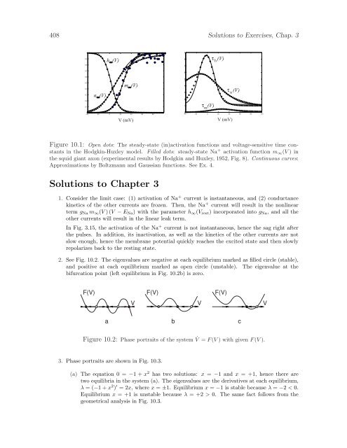
- Page 420 and 421: 410 Solutions to Exercises, Chap. 3
- Page 422 and 423: 412 Solutions to Exercises, Chap. 3
- Page 424 and 425: 414 Solutions to Exercises, Chap. 4
- Page 426 and 427: 416 Solutions to Exercises, Chap. 4
- Page 428 and 429: 418 Solutions to Exercises, Chap. 4
- Page 430 and 431: 420 Solutions to Exercises, Chap. 4
- Page 432 and 433: 422 Solutions to Exercises, Chap. 5
- Page 434 and 435: 424 Solutions to Exercises, Chap. 6
- Page 436 and 437: 426 Solutions to Exercises, Chap. 6
- Page 438 and 439: 428 Solutions to Exercises, Chap. 8
- Page 440 and 441: 430 Solutions to Exercises, Chap. 9
- Page 442 and 443: 432 Solutions to Exercises, Chap. 9
- Page 444 and 445: 434 Solutions to Exercises, Chap. 9
- Page 446 and 447: 436 Solutions to Exercises, Chap. 9
- Page 448 and 449: 438 Solutions to Exercises, Chap. 9
- Page 450 and 451: 440 Solutions to Exercises, Chap. 9
- Page 452 and 453: 442 Referencesterneurons mediated b
- Page 454 and 455: 444 ReferencesDickson C.T., Magistr
- Page 456 and 457: 446 ReferencesGuckenheimer J. (1975
- Page 458 and 459: 448 Referencestional Journal of Bif
- Page 460 and 461: 450 ReferencesMarkram H, Toledo-Rod
- Page 462 and 463: 452 ReferencesRosenblum M.G. and Pi
- Page 464 and 465: 454 ReferencesTuckwell H.C. (1988)
- Page 466 and 467: 456 References9
- Page 468 and 469:
458 Synchronization (see www.izhike
- Page 470 and 471:
460 Synchronization (see www.izhike
- Page 472 and 473:
462 Synchronization (see www.izhike
- Page 474 and 475:
464 Synchronization (see www.izhike
- Page 476 and 477:
466 Synchronization (see www.izhike
- Page 478 and 479:
468 Synchronization (see www.izhike
- Page 480 and 481:
470 Synchronization (see www.izhike
- Page 482 and 483:
472 Synchronization (see www.izhike
- Page 484 and 485:
474 Synchronization (see www.izhike
- Page 486 and 487:
476 Synchronization (see www.izhike
- Page 488 and 489:
478 Synchronization (see www.izhike
- Page 490 and 491:
480 Synchronization (see www.izhike
- Page 492 and 493:
482 Synchronization (see www.izhike
- Page 494 and 495:
484 Synchronization (see www.izhike
- Page 496 and 497:
486 Synchronization (see www.izhike
- Page 498 and 499:
488 Synchronization (see www.izhike
- Page 500 and 501:
490 Synchronization (see www.izhike
- Page 502 and 503:
492 Synchronization (see www.izhike
- Page 504 and 505:
494 Synchronization (see www.izhike
- Page 506 and 507:
496 Synchronization (see www.izhike
- Page 508 and 509:
498 Synchronization (see www.izhike
- Page 510 and 511:
500 Synchronization (see www.izhike
- Page 512 and 513:
502 Synchronization (see www.izhike
- Page 514 and 515:
504 Synchronization (see www.izhike
- Page 516 and 517:
506 Synchronization (see www.izhike
- Page 518 and 519:
508 Synchronization (see www.izhike
- Page 520 and 521:
510 Synchronization (see www.izhike
- Page 522 and 523:
512 Solutions to Exercises, Chap. 1
- Page 524 and 525:
514 Solutions to Exercises, Chap. 1
- Page 526 and 527:
516 Solutions to Exercises, Chap. 1
- Page 528:
518 Solutions to Exercises, Chap. 1