Dynamical Systems in Neuroscience:

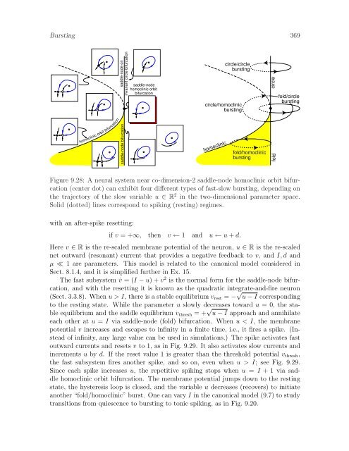
Bursting 369homoclinic orbit bifurcationsaddle-node bifurcation saddle-node oninvariant circle bifurcationsaddle-nodehomoclinic orbitbifurcationcircle/homoclinicburstinghomocliniccircle/circleburstingfold/homoclinicburstingcirclefoldfold/circleburstingFigure 9.28: A neural system near co-dimension-2 saddle-node homoclinic orbit bifurcation(center dot) can exhibit four different types of fast-slow bursting, depending onthe trajectory of the slow variable u ∈ R 2 in the two-dimensional parameter space.Solid (dotted) lines correspond to spiking (resting) regimes.with an after-spike resetting:if v = +∞, then v ← 1 and u ← u + d.Here v ∈ R is the re-scaled membrane potential of the neuron, u ∈ R is the re-scalednet outward (resonant) current that provides a negative feedback to v, and I, d andµ ≪ 1 are parameters. This model is related to the canonical model considered inSect. 8.1.4, and it is simplified further in Ex. 15.The fast subsystem ˙v = (I − u) + v 2 is the normal form for the saddle-node bifurcation,and with the resetting it is known as the quadratic integrate-and-fire neuron(Sect. 3.3.8). When u > I, there is a stable equilibrium v rest = − √ u − I correspondingto the resting state. While the parameter u slowly decreases toward u = 0, the stableequilibrium and the saddle equilibrium v thresh = + √ u − I approach and annihilateeach other at u = I via saddle-node (fold) bifurcation. When u < I, the membranepotential v increases and escapes to infinity in a finite time, i.e., it fires a spike. (Insteadof infinity, any large value can be used in simulations.) The spike activates fastoutward currents and resets v to 1, as in Fig. 9.29. It also activates slow currents andincrements u by d. If the reset value 1 is greater than the threshold potential v thresh ,the fast subsystem fires another spike, and so on, even when u > I; see Fig. 9.29.Since each spike increases u, the repetitive spiking stops when u = I + 1 via saddlehomoclinic orbit bifurcation. The membrane potential jumps down to the restingstate, the hysteresis loop is closed, and the variable u decreases (recovers) to initiateanother “fold/homoclinic” burst. One can vary I in the canonical model (9.7) to studytransitions from quiescence to bursting to tonic spiking, as in Fig. 9.20.