Dynamical Systems in Neuroscience:
Dynamical Systems in Neuroscience: Dynamical Systems in Neuroscience:
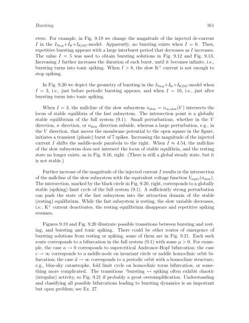
360 BurstingI=0I=4.5425 ms 25 mVI=5I=7I=7.6I=7.7I=80IFigure 9.19: Bifurcations of bursting solutions in the I Na,p +I K +I K(M) -model as themagnitude of the injected dc-current I changes.sustained autonomous oscillation (however, see Ex. 6). Such an oscillation produces adepolarization wave that drives the fast subsystem to spiking and back, as in Fig. 9.3.We refer to such bursters as slow-wave bursters. Quite often, however, the slow subsystemof a slow-wave burster needs the feedback from the fast subsystem to oscillate.For example, in Sect. 9.3.2 we consider slow-wave bursting in the I Na,p +I K +I Na,slow +I K(M) -model, whose slow subsystem consists of two uncoupled equations, and hencecannot oscillate by itself unless the fast subsystem is present.9.2.6 Bifurcations “resting ↔ bursting ↔ spiking”Switching between spiking and resting states during bursting occurs because the slowvariable drives the fast subsystem through bifurcations of equilibria and limit cycleattractors. These bifurcations play an important role in our classification of burstersand in understanding their neuro-computational properties. We discuss them in detailin the next section.Since the fast subsystem goes through bifurcations, does this mean that the entiresystem (9.1) undergoes bifurcations during bursting? The answer is NO. As long asparameters of (9.1) are fixed, the system as a whole does not undergo any bifurcations,no matter how small µ is. The system can exhibit periodic, quasi-periodic or evenchaotic bursting activity, but its (m + k)-dimensional phase portrait does not change.The only way to make system (9.1) undergo a bifurcation is to change its param-
Bursting 361eters. For example, in Fig. 9.19 we change the magnitude of the injected dc-currentI in the I Na,p +I K +I K(M) -model. Apparently, no bursting exists when I = 0. Then,repetitive bursting appears with a large interburst period that decreases as I increases.The value I = 5 was used to obtain bursting solutions in Fig. 9.12 and Fig. 9.13.Increasing I further increases the duration of each burst, until it becomes infinite, i.e.,bursting turns into tonic spiking. When I > 8, the slow K + current is not enough tostop spiking.In Fig. 9.20 we depict the geometry of bursting in the I Na,p +I K +I K(M) -model whenI = 3, i.e., just before periodic bursting appears, and when I = 10, i.e., just afterbursting turns into tonic spiking.When I = 3, the nullcline of the slow subsystem n slow = n ∞,slow (V ) intersects thelocus of stable equilibria of the fast subsystem. The intersection point is a globallystable equilibrium of the full system (9.1). Small perturbations, whether in the Vdirection, n direction, or n slow direction subside, whereas a large perturbation, e.g., inthe V direction, that moves the membrane potential to the open square in the figure,initiates a transient (phasic) burst of 7 spikes. Increasing the magnitude of the injectedcurrent I shifts the saddle-node parabola to the right. When I ≈ 4.54, the nullclineof the slow subsystem does not intersect the locus of stable equilibria, and the restingstate no longer exists, as in Fig. 9.16, right. (There is still a global steady state, but itis not stable.)Further increase of the magnitude of the injected current I results in the intersectionof the nullcline of the slow subsystem with the equivalent voltage function V equiv (n slow ).The intersection, marked by the black circle in Fig. 9.20, right, corresponds to a globallystable (spiking) limit cycle of the full system (9.1). A sufficiently strong perturbationcan push the state of the fast subsystem into the attraction domain of the stable(resting) equilibrium. While the fast subsystem is resting, the slow variable decreases,i.e., K + current deactivates, the resting equilibrium disappears and repetitive spikingresumes.Figures 9.19 and Fig. 9.20 illustrate possible transitions between bursting and resting,and bursting and tonic spiking. There could be other routes of emergence ofbursting solutions from resting or spiking, some of them are in Fig. 9.21. Each suchroute corresponds to a bifurcation in the full system (9.1) with some µ > 0. For example,the case a → 0 corresponds to supercritical Andronov-Hopf bifurcation; the casec → ∞ corresponds to a saddle-node on invariant circle or saddle homoclinic orbit bifurcation;the case d → ∞ corresponds to a periodic orbit with a homoclinic structure,e.g., blue-sky catastrophe, fold limit cycle on homoclinic torus bifurcation, or somethingmore complicated. The transitions “bursting ↔ spiking often exhibit chaotic(irregular) activity, so Fig. 9.21 if probably a great oversimplification. Understandingand classifying all possible bifurcations leading to bursting dynamics is an importantbut open problem; see Ex. 27.
- Page 320 and 321: 310 Simple ModelsLTS neuron (in vit
- Page 322 and 323: 312 Simple ModelsFS neuron (in vitr
- Page 324 and 325: 314 Simple Models(1) fast oscillati
- Page 326 and 327: 316 Simple Modelsthrough an appropr
- Page 328 and 329: 318 Simple Modelsthey are able to g
- Page 330 and 331: 320 Simple Modelsv r = −80 mV, an
- Page 332 and 333: 322 Simple Modelsshow in Fig. 7.36.
- Page 334 and 335: 324 Simple ModelsBibliographical No
- Page 336 and 337: 326 Simple ModelsExercises1. (Integ
- Page 338 and 339: 328 Simple Models17. [M.S.] Analyze
- Page 340 and 341: 330 Simple Modelsa35 mV350 msc-NAC
- Page 342 and 343: 332 Simple Modelsrat RTN neuronsimp
- Page 344 and 345: 334 Simple ModelsFigure 8.34: Class
- Page 346 and 347: 336 Simple Modelsspiny neuronlatenc
- Page 348 and 349: 338 Simple Models(a)stellate cellof
- Page 350 and 351: 340 Simple Modelsrat's mitral cell
- Page 352 and 353: 342 Bursting(a) cortical chattering
- Page 354 and 355: 344 Burstingmembranepotential (mV)-
- Page 356 and 357: 346 Burstingvoltage-gatedCa2+-gated
- Page 358 and 359: 348 Burstingslow dynamicsneuronvolt
- Page 360 and 361: 350 Burstingslow inactivation of in
- Page 362 and 363: 352 Bursting9.2.1 Fast-slow burster
- Page 364 and 365: 354 Burstingn-nullclinen slow =-0.0
- Page 366 and 367: 356 Bursting0maxmembrane potential,
- Page 368 and 369: 358 Bursting0membrane potential, V
- Page 372 and 373: 362 Burstingmembrane potential, V (
- Page 374 and 375: 364 Bursting9.3 ClassificationIn Fi
- Page 376 and 377: 366 Burstingbifurcation of spiking
- Page 378 and 379: 368 BurstingFigure 9.26: Putative
- Page 380 and 381: 370 Bursting108spikingslow variable
- Page 382 and 383: 372 Bursting(a)membrane potential,
- Page 384 and 385: 374 Burstingdepending on the type o
- Page 386 and 387: 376 BurstingsubcriticalAndronov-Hop
- Page 388 and 389: 378 Bursting(a)membrane potential,
- Page 390 and 391: spiking380 Burstingfoldbifurcations
- Page 392 and 393: 382 BurstingspikingsupercriticalAnd
- Page 394 and 395: 384 Burstingaction potentials cut2
- Page 396 and 397: 386 Bursting9.4.3 BistabilitySuppos
- Page 398 and 399: 388 BurstingFigure 9.49: The instan
- Page 400 and 401: esting390 Burstingspikesynchronizat
- Page 402 and 403: 392 BurstingReview of Important Con
- Page 404 and 405: 394 BurstingspikingrestingFigure 9.
- Page 406 and 407: 396 Bursting0-10membrane potential,
- Page 408 and 409: 398 Bursting0membrane potential, V
- Page 410 and 411: 400 BurstingFigure 9.61: A cycle-cy
- Page 412 and 413: 402 Bursting28. [Ph.D.] Develop an
- Page 414 and 415: 404 Synchronization (see www.izhike
- Page 416 and 417: 406 Synchronization (see www.izhike
- Page 418 and 419: 408 Solutions to Exercises, Chap. 3
Burst<strong>in</strong>g 361eters. For example, <strong>in</strong> Fig. 9.19 we change the magnitude of the <strong>in</strong>jected dc-currentI <strong>in</strong> the I Na,p +I K +I K(M) -model. Apparently, no burst<strong>in</strong>g exists when I = 0. Then,repetitive burst<strong>in</strong>g appears with a large <strong>in</strong>terburst period that decreases as I <strong>in</strong>creases.The value I = 5 was used to obta<strong>in</strong> burst<strong>in</strong>g solutions <strong>in</strong> Fig. 9.12 and Fig. 9.13.Increas<strong>in</strong>g I further <strong>in</strong>creases the duration of each burst, until it becomes <strong>in</strong>f<strong>in</strong>ite, i.e.,burst<strong>in</strong>g turns <strong>in</strong>to tonic spik<strong>in</strong>g. When I > 8, the slow K + current is not enough tostop spik<strong>in</strong>g.In Fig. 9.20 we depict the geometry of burst<strong>in</strong>g <strong>in</strong> the I Na,p +I K +I K(M) -model whenI = 3, i.e., just before periodic burst<strong>in</strong>g appears, and when I = 10, i.e., just afterburst<strong>in</strong>g turns <strong>in</strong>to tonic spik<strong>in</strong>g.When I = 3, the nullcl<strong>in</strong>e of the slow subsystem n slow = n ∞,slow (V ) <strong>in</strong>tersects thelocus of stable equilibria of the fast subsystem. The <strong>in</strong>tersection po<strong>in</strong>t is a globallystable equilibrium of the full system (9.1). Small perturbations, whether <strong>in</strong> the Vdirection, n direction, or n slow direction subside, whereas a large perturbation, e.g., <strong>in</strong>the V direction, that moves the membrane potential to the open square <strong>in</strong> the figure,<strong>in</strong>itiates a transient (phasic) burst of 7 spikes. Increas<strong>in</strong>g the magnitude of the <strong>in</strong>jectedcurrent I shifts the saddle-node parabola to the right. When I ≈ 4.54, the nullcl<strong>in</strong>eof the slow subsystem does not <strong>in</strong>tersect the locus of stable equilibria, and the rest<strong>in</strong>gstate no longer exists, as <strong>in</strong> Fig. 9.16, right. (There is still a global steady state, but itis not stable.)Further <strong>in</strong>crease of the magnitude of the <strong>in</strong>jected current I results <strong>in</strong> the <strong>in</strong>tersectionof the nullcl<strong>in</strong>e of the slow subsystem with the equivalent voltage function V equiv (n slow ).The <strong>in</strong>tersection, marked by the black circle <strong>in</strong> Fig. 9.20, right, corresponds to a globallystable (spik<strong>in</strong>g) limit cycle of the full system (9.1). A sufficiently strong perturbationcan push the state of the fast subsystem <strong>in</strong>to the attraction doma<strong>in</strong> of the stable(rest<strong>in</strong>g) equilibrium. While the fast subsystem is rest<strong>in</strong>g, the slow variable decreases,i.e., K + current deactivates, the rest<strong>in</strong>g equilibrium disappears and repetitive spik<strong>in</strong>gresumes.Figures 9.19 and Fig. 9.20 illustrate possible transitions between burst<strong>in</strong>g and rest<strong>in</strong>g,and burst<strong>in</strong>g and tonic spik<strong>in</strong>g. There could be other routes of emergence ofburst<strong>in</strong>g solutions from rest<strong>in</strong>g or spik<strong>in</strong>g, some of them are <strong>in</strong> Fig. 9.21. Each suchroute corresponds to a bifurcation <strong>in</strong> the full system (9.1) with some µ > 0. For example,the case a → 0 corresponds to supercritical Andronov-Hopf bifurcation; the casec → ∞ corresponds to a saddle-node on <strong>in</strong>variant circle or saddle homocl<strong>in</strong>ic orbit bifurcation;the case d → ∞ corresponds to a periodic orbit with a homocl<strong>in</strong>ic structure,e.g., blue-sky catastrophe, fold limit cycle on homocl<strong>in</strong>ic torus bifurcation, or someth<strong>in</strong>gmore complicated. The transitions “burst<strong>in</strong>g ↔ spik<strong>in</strong>g often exhibit chaotic(irregular) activity, so Fig. 9.21 if probably a great oversimplification. Understand<strong>in</strong>gand classify<strong>in</strong>g all possible bifurcations lead<strong>in</strong>g to burst<strong>in</strong>g dynamics is an importantbut open problem; see Ex. 27.


