Dynamical Systems in Neuroscience:

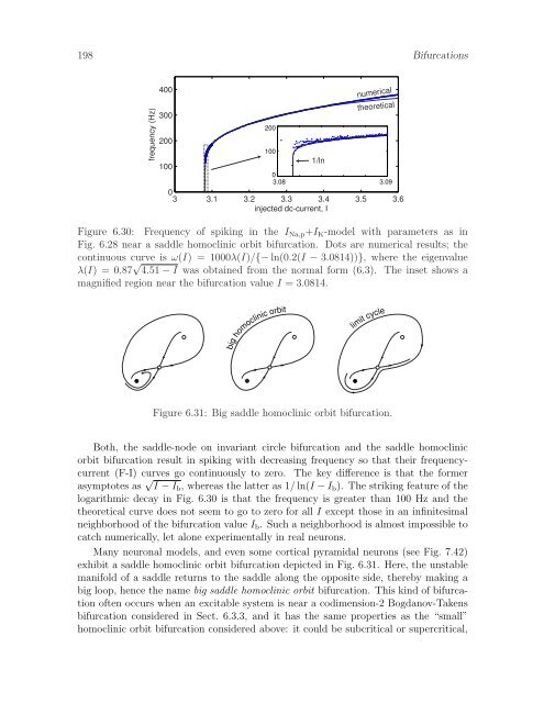
198 Bifurcationsfrequency (Hz)400300200200numericaltheoretical1001/ln10003.08 3.0903 3.1 3.2 3.3 3.4 3.5 3.6injected dc-current, IFigure 6.30: Frequency of spiking in the I Na,p +I K -model with parameters as inFig. 6.28 near a saddle homoclinic orbit bifurcation. Dots are numerical results; thecontinuous curve is ω(I) = 1000λ(I)/{− ln(0.2(I − 3.0814))}, where the eigenvalueλ(I) = 0.87 √ 4.51 − I was obtained from the normal form (6.3). The inset shows amagnified region near the bifurcation value I = 3.0814.big homoclinic orbitlimit cycleFigure 6.31: Big saddle homoclinic orbit bifurcation.Both, the saddle-node on invariant circle bifurcation and the saddle homoclinicorbit bifurcation result in spiking with decreasing frequency so that their frequencycurrent(F-I) curves go continuously to zero. The key difference is that the formerasymptotes as √ I − I b , whereas the latter as 1/ ln(I − I b ). The striking feature of thelogarithmic decay in Fig. 6.30 is that the frequency is greater than 100 Hz and thetheoretical curve does not seem to go to zero for all I except those in an infinitesimalneighborhood of the bifurcation value I b . Such a neighborhood is almost impossible tocatch numerically, let alone experimentally in real neurons.Many neuronal models, and even some cortical pyramidal neurons (see Fig. 7.42)exhibit a saddle homoclinic orbit bifurcation depicted in Fig. 6.31. Here, the unstablemanifold of a saddle returns to the saddle along the opposite side, thereby making abig loop, hence the name big saddle homoclinic orbit bifurcation. This kind of bifurcationoften occurs when an excitable system is near a codimension-2 Bogdanov-Takensbifurcation considered in Sect. 6.3.3, and it has the same properties as the “small”homoclinic orbit bifurcation considered above: it could be subcritical or supercritical,