Dynamical Systems in Neuroscience:

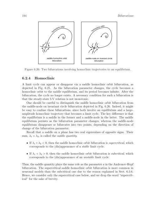
194 Bifurcationshomoclinic orbithomoclinic orbitsaddle homoclinic orbitbifurcationsaddle-node on invariant circlebifurcationFigure 6.26: Two bifurcations involving homoclinic trajectories to an equilibrium.6.2.4 HomoclinicA limit cycle can appear or disappear via a saddle homoclinic orbit bifurcation, asdepicted in Fig. 6.25. As the bifurcation parameter changes, the cycle becomes ahomoclinic orbit to the saddle equilibrium, and its period becomes infinite. After thebifurcation, the cycle no longer exists. A necessary condition for such a bifurcation isthat the steady-state I-V relation is not monotonic.One should be careful to distinguish the saddle homoclinic orbit bifurcation fromthe saddle-node on invariant circle bifurcation depicted in Fig. 6.26. Indeed, it mightbe easy to confuse these bifurcations, since both involve an equilibrium and a largeamplitudehomoclinic trajectory that becomes a limit cycle. The key difference is thatthe equilibrium is a saddle in the former and a saddle-node in the latter. The saddleequilibrium persists as the bifurcation parameter changes, whereas the saddle-nodeequilibrium disappears or bifurcates into two points, depending on the direction ofchange of the bifurcation parameter.Recall that a saddle on a plane has two real eigenvalues of opposite signs. Theirsum, λ 1 + λ 2 , is called the saddle quantity.• If λ 1 + λ 2 < 0, then the saddle homoclinic orbit bifurcation is supercritical, whichcorresponds to the (dis)appearance of a stable limit cycle.• If λ 1 + λ 2 > 0, then the saddle homoclinic orbit bifurcation is subcritical, whichcorresponds to the (dis)appearance of an unstable limit cycle.Thus, the saddle quantity plays the same role as the parameter a in the Andronov-Hopfbifurcation. The supercritical saddle homoclinic orbit bifurcation is more common inneuronal models than the subcritical one due to the reason explained in Sect. 6.3.6.Hence, we consider only the supercritical case below, and we drop the word “supercritical”for the sake of brevity.