Dynamical Systems in Neuroscience:

Eugene M. IzhikevichThe Neurosciences InstituteDynamical Systems in Neuroscience:The Geometry of Excitability and BurstingDecember 19, 2005The MIT Press

4.3.1 Bistability and attraction domains . . . . . . . . . . . . . . . . 1134.3.2 Stable/unstable manifolds . . . . . . . . . . . . . . . . . . . . . 1144.3.3 Homoclinic/heteroclinic trajectories . . . . . . . . . . . . . . . . 1164.3.4 Saddle-node bifurcation . . . . . . . . . . . . . . . . . . . . . . 1164.3.5 Andronov-Hopf bifurcation . . . . . . . . . . . . . . . . . . . . . 122Summary and Bibliographical Notes . . . . . . . . . . . . . . . . . . . . . . 124Exercises . . . . . . . . . . . . . . . . . . . . . . . . . . . . . . . . . . . . . . 1275 Conductance-Based Models and Their Reductions 1335.1 Minimal Models . . . . . . . . . . . . . . . . . . . . . . . . . . . . . . . 1335.1.1 Amplifying and resonant gating variables . . . . . . . . . . . . . 1355.1.2 I Na,p +I K -model . . . . . . . . . . . . . . . . . . . . . . . . . . . 1385.1.3 I Na,t -model . . . . . . . . . . . . . . . . . . . . . . . . . . . . . 1395.1.4 I Na,p +I h -model . . . . . . . . . . . . . . . . . . . . . . . . . . . 1425.1.5 I h +I Kir -model . . . . . . . . . . . . . . . . . . . . . . . . . . . . 1445.1.6 I K +I Kir -model . . . . . . . . . . . . . . . . . . . . . . . . . . . . 1455.1.7 I A -model . . . . . . . . . . . . . . . . . . . . . . . . . . . . . . . 1485.1.8 Ca 2+ -gated minimal models . . . . . . . . . . . . . . . . . . . . 1525.2 Reduction of multi-dimensional models . . . . . . . . . . . . . . . . . . 1555.2.1 Hodgkin-Huxley model . . . . . . . . . . . . . . . . . . . . . . . 1555.2.2 Equivalent potentials . . . . . . . . . . . . . . . . . . . . . . . . 1585.2.3 Nullclines and I-V recordings . . . . . . . . . . . . . . . . . . . 1585.2.4 Reduction to simple model . . . . . . . . . . . . . . . . . . . . . 161Summary and Bibliographical Notes . . . . . . . . . . . . . . . . . . . . . . 163Exercises . . . . . . . . . . . . . . . . . . . . . . . . . . . . . . . . . . . . . . 1646 Bifurcations 1676.1 Equilibrium (Rest State) . . . . . . . . . . . . . . . . . . . . . . . . . . 1676.1.1 Saddle-node (fold) . . . . . . . . . . . . . . . . . . . . . . . . . 1706.1.2 Saddle-node on invariant circle . . . . . . . . . . . . . . . . . . 1736.1.3 Supercritical Andronov-Hopf . . . . . . . . . . . . . . . . . . . . 1776.1.4 Subcritical Andronov-Hopf . . . . . . . . . . . . . . . . . . . . . 1816.2 Limit Cycle (Spiking State) . . . . . . . . . . . . . . . . . . . . . . . . 1866.2.1 Saddle-node on invariant circle . . . . . . . . . . . . . . . . . . 1886.2.2 Supercritical Andronov-Hopf . . . . . . . . . . . . . . . . . . . . 1896.2.3 Fold limit cycle . . . . . . . . . . . . . . . . . . . . . . . . . . . 1906.2.4 Homoclinic . . . . . . . . . . . . . . . . . . . . . . . . . . . . . 1946.3 Other Interesting Cases . . . . . . . . . . . . . . . . . . . . . . . . . . . 1996.3.1 Three-dimensional phase space . . . . . . . . . . . . . . . . . . 1996.3.2 Cusp and pitchfork . . . . . . . . . . . . . . . . . . . . . . . . . 2016.3.3 Bogdanov-Takens . . . . . . . . . . . . . . . . . . . . . . . . . . 2026.3.4 Relaxation oscillators and Canards . . . . . . . . . . . . . . . . 2076.3.5 Bautin . . . . . . . . . . . . . . . . . . . . . . . . . . . . . . . . 209

6.3.6 Saddle-node homoclinic orbit . . . . . . . . . . . . . . . . . . . 2106.3.7 Hard and soft loss of stability . . . . . . . . . . . . . . . . . . . 213Summary and Bibliographical Notes . . . . . . . . . . . . . . . . . . . . . . 214Exercises . . . . . . . . . . . . . . . . . . . . . . . . . . . . . . . . . . . . . . 2207 Neuronal Excitability 2257.1 Excitability . . . . . . . . . . . . . . . . . . . . . . . . . . . . . . . . . 2257.1.1 Bifurcations . . . . . . . . . . . . . . . . . . . . . . . . . . . . . 2267.1.2 Hodgkin’s classification . . . . . . . . . . . . . . . . . . . . . . . 2287.1.3 Classes 1 and 2 . . . . . . . . . . . . . . . . . . . . . . . . . . . 2317.1.4 Class 3 . . . . . . . . . . . . . . . . . . . . . . . . . . . . . . . . 2327.1.5 Ramps, steps, and shocks . . . . . . . . . . . . . . . . . . . . . 2347.1.6 Bistability . . . . . . . . . . . . . . . . . . . . . . . . . . . . . . 2367.1.7 Class 1 and 2 spiking . . . . . . . . . . . . . . . . . . . . . . . . 2387.2 Integrators vs. Resonators . . . . . . . . . . . . . . . . . . . . . . . . . 2397.2.1 Fast subthreshold oscillations . . . . . . . . . . . . . . . . . . . 2407.2.2 Frequency preference and resonance . . . . . . . . . . . . . . . . 2427.2.3 Frequency preference in vivo . . . . . . . . . . . . . . . . . . . . 2477.2.4 Thresholds and action potentials . . . . . . . . . . . . . . . . . 2497.2.5 Threshold manifolds . . . . . . . . . . . . . . . . . . . . . . . . 2507.2.6 Rheobase . . . . . . . . . . . . . . . . . . . . . . . . . . . . . . 2527.2.7 Post-inhibitory spike . . . . . . . . . . . . . . . . . . . . . . . . 2537.2.8 Inhibition-induced spiking . . . . . . . . . . . . . . . . . . . . . 2557.2.9 Spike latency . . . . . . . . . . . . . . . . . . . . . . . . . . . . 2577.2.10 Flipping from an integrator to a resonator . . . . . . . . . . . . 2597.2.11 Transition between integrators and resonators . . . . . . . . . . 2617.3 Slow Modulation . . . . . . . . . . . . . . . . . . . . . . . . . . . . . . 2647.3.1 Spike-frequency modulation . . . . . . . . . . . . . . . . . . . . 2657.3.2 I-V relation . . . . . . . . . . . . . . . . . . . . . . . . . . . . . 2677.3.3 Slow Subthreshold oscillation . . . . . . . . . . . . . . . . . . . 2707.3.4 Rebound response and voltage sag . . . . . . . . . . . . . . . . 2707.3.5 AHP and ADP . . . . . . . . . . . . . . . . . . . . . . . . . . . 272Summary and Bibliographical Notes . . . . . . . . . . . . . . . . . . . . . . 274Exercises . . . . . . . . . . . . . . . . . . . . . . . . . . . . . . . . . . . . . . 2768 Simple Models 2798.1 Simplest Models . . . . . . . . . . . . . . . . . . . . . . . . . . . . . . . 2798.1.1 Integrate-and-fire . . . . . . . . . . . . . . . . . . . . . . . . . . 2808.1.2 Resonate-and-fire . . . . . . . . . . . . . . . . . . . . . . . . . . 2818.1.3 Quadratic integrate-and-fire . . . . . . . . . . . . . . . . . . . . 2828.1.4 Simple model of choice . . . . . . . . . . . . . . . . . . . . . . . 2838.1.5 Canonical models . . . . . . . . . . . . . . . . . . . . . . . . . . 2898.2 Cortex . . . . . . . . . . . . . . . . . . . . . . . . . . . . . . . . . . . . 292

8.2.1 Regular spiking (RS) neurons . . . . . . . . . . . . . . . . . . . 2958.2.2 Intrinsically bursting (IB) neurons . . . . . . . . . . . . . . . . . 3018.2.3 Multi-compartment dendritic tree . . . . . . . . . . . . . . . . . 3058.2.4 Chattering (CH) neurons . . . . . . . . . . . . . . . . . . . . . . 3078.2.5 Low-threshold spiking (LTS) interneurons . . . . . . . . . . . . 3088.2.6 Fast spiking (FS) interneurons . . . . . . . . . . . . . . . . . . . 3118.2.7 Late spiking (LS) interneurons . . . . . . . . . . . . . . . . . . . 3138.2.8 Diversity of inhibitory interneurons . . . . . . . . . . . . . . . . 3148.3 Thalamus . . . . . . . . . . . . . . . . . . . . . . . . . . . . . . . . . . 3158.3.1 Thalamo-cortical (TC) relay neurons . . . . . . . . . . . . . . . 3168.3.2 Reticular thalamic nucleus (RTN) neurons . . . . . . . . . . . . 3178.3.3 Thalamic interneurons . . . . . . . . . . . . . . . . . . . . . . . 3178.4 Other interesting cases . . . . . . . . . . . . . . . . . . . . . . . . . . . 3188.4.1 Hippocampal CA1 pyramidal neurons . . . . . . . . . . . . . . . 3188.4.2 Spiny projection neurons of neostriatum and basal ganglia . . . 3198.4.3 Mesencephalic V neurons of brainstem . . . . . . . . . . . . . . 3208.4.4 Stellate cells of entorhinal cortex . . . . . . . . . . . . . . . . . 3208.4.5 Mitral neurons of olfactory bulb . . . . . . . . . . . . . . . . . . 321Summary and Bibliographical Notes . . . . . . . . . . . . . . . . . . . . . . 323Exercises . . . . . . . . . . . . . . . . . . . . . . . . . . . . . . . . . . . . . . 3269 Bursting 3419.1 Electrophysiology . . . . . . . . . . . . . . . . . . . . . . . . . . . . . . 3419.1.1 Example: The I Na,p +I K +I K(M) -model . . . . . . . . . . . . . . . 3439.1.2 Fast-Slow Dynamics . . . . . . . . . . . . . . . . . . . . . . . . 3459.1.3 Minimal models . . . . . . . . . . . . . . . . . . . . . . . . . . . 3479.1.4 Central pattern generators and half-center oscillators . . . . . . 3519.2 Geometry . . . . . . . . . . . . . . . . . . . . . . . . . . . . . . . . . . 3519.2.1 Fast-slow bursters . . . . . . . . . . . . . . . . . . . . . . . . . . 3529.2.2 Phase portraits . . . . . . . . . . . . . . . . . . . . . . . . . . . 3529.2.3 Averaging . . . . . . . . . . . . . . . . . . . . . . . . . . . . . . 3559.2.4 Equivalent voltage . . . . . . . . . . . . . . . . . . . . . . . . . 3579.2.5 Hysteresis loops and slow waves . . . . . . . . . . . . . . . . . . 3589.2.6 Bifurcations “resting ↔ bursting ↔ spiking” . . . . . . . . . . . 3609.3 Classification . . . . . . . . . . . . . . . . . . . . . . . . . . . . . . . . 3649.3.1 fold/homoclinic . . . . . . . . . . . . . . . . . . . . . . . . . . . 3659.3.2 circle/circle . . . . . . . . . . . . . . . . . . . . . . . . . . . . . 3719.3.3 subHopf/fold cycle . . . . . . . . . . . . . . . . . . . . . . . . . 3749.3.4 fold/fold cycle . . . . . . . . . . . . . . . . . . . . . . . . . . . . 3819.3.5 fold/Hopf . . . . . . . . . . . . . . . . . . . . . . . . . . . . . . 3819.3.6 fold/circle . . . . . . . . . . . . . . . . . . . . . . . . . . . . . . 3819.4 Neuro-Computational Properties . . . . . . . . . . . . . . . . . . . . . 3839.4.1 How to distinguish? . . . . . . . . . . . . . . . . . . . . . . . . . 383

9.4.2 Integrators vs. Resonators . . . . . . . . . . . . . . . . . . . . . 3849.4.3 Bistability . . . . . . . . . . . . . . . . . . . . . . . . . . . . . . 3869.4.4 Bursts as a unit of neuronal information . . . . . . . . . . . . . 3879.4.5 Synchronization . . . . . . . . . . . . . . . . . . . . . . . . . . . 389Summary and Bibliographical Notes . . . . . . . . . . . . . . . . . . . . . . 392Exercises . . . . . . . . . . . . . . . . . . . . . . . . . . . . . . . . . . . . . . 39510 Synchronization (see www.izhikevich.com) 403Solutions to Exercises 407References 44110 Synchronization (see www.izhikevich.com) 45710.1 Pulsed Coupling . . . . . . . . . . . . . . . . . . . . . . . . . . . . . . . 45710.1.1 Phase of oscillation . . . . . . . . . . . . . . . . . . . . . . . . . 45810.1.2 Isochrons . . . . . . . . . . . . . . . . . . . . . . . . . . . . . . 45910.1.3 PRC . . . . . . . . . . . . . . . . . . . . . . . . . . . . . . . . . 46010.1.4 Type 0 and 1 phase response . . . . . . . . . . . . . . . . . . . . 46310.1.5 Poincare phase map . . . . . . . . . . . . . . . . . . . . . . . . 46610.1.6 Fixed points . . . . . . . . . . . . . . . . . . . . . . . . . . . . . 46710.1.7 Synchronization . . . . . . . . . . . . . . . . . . . . . . . . . . . 46810.1.8 Phase locking . . . . . . . . . . . . . . . . . . . . . . . . . . . . 46910.1.9 Arnold tongues . . . . . . . . . . . . . . . . . . . . . . . . . . . 47010.2 Weak Coupling . . . . . . . . . . . . . . . . . . . . . . . . . . . . . . . 47110.2.1 Winfree’s approach . . . . . . . . . . . . . . . . . . . . . . . . . 47210.2.2 Kuramoto’s approach . . . . . . . . . . . . . . . . . . . . . . . . 47410.2.3 Malkin’s approach . . . . . . . . . . . . . . . . . . . . . . . . . 47510.2.4 Measuring PRCs experimentally . . . . . . . . . . . . . . . . . . 47610.2.5 Phase model for coupled oscillators . . . . . . . . . . . . . . . . 47910.3 Synchronization . . . . . . . . . . . . . . . . . . . . . . . . . . . . . . . 48110.3.1 Two oscillators . . . . . . . . . . . . . . . . . . . . . . . . . . . 48310.3.2 Chains . . . . . . . . . . . . . . . . . . . . . . . . . . . . . . . . 48510.3.3 Networks . . . . . . . . . . . . . . . . . . . . . . . . . . . . . . 48710.3.4 Mean-field approximations . . . . . . . . . . . . . . . . . . . . . 48810.4 Examples . . . . . . . . . . . . . . . . . . . . . . . . . . . . . . . . . . 48910.4.1 Phase oscillators . . . . . . . . . . . . . . . . . . . . . . . . . . 48910.4.2 SNIC oscillators . . . . . . . . . . . . . . . . . . . . . . . . . . . 49010.4.3 Homoclinic oscillators . . . . . . . . . . . . . . . . . . . . . . . 49610.4.4 Relaxation oscillators and FTM . . . . . . . . . . . . . . . . . . 49810.4.5 Bursting oscillators . . . . . . . . . . . . . . . . . . . . . . . . . 500Summary and Bibliographical Notes . . . . . . . . . . . . . . . . . . . . . . 501Exercises . . . . . . . . . . . . . . . . . . . . . . . . . . . . . . . . . . . . . . 506Solutions . . . . . . . . . . . . . . . . . . . . . . . . . . . . . . . . . . . . . . 511

PrefaceHistorically, much of theoretical neuroscience research concerned neuronal circuits andsynaptic organization. The neurons were divided into excitatory and inhibitory types,but their electrophysiological properties were largely neglected or taken to be identicalto those of Hodgkin-Huxley’s squid axon. The present awareness of the importance ofthe electrophysiology of individual neurons is best summarized by David McCormick inthe fifth edition of Gordon Shepherd’s book “The Synaptic Organization of the Brain”:“Information processing depends not only on the anatomical substrates of synapticcircuits but also on the electrophysiological properties of neurons... . Even iftwo neurons in different regions of the nervous system possess identical morphologicalfeatures, they may respond to the same synaptic input in very differentmanners because of each cell’s intrinsic properties.”David A. McCormick (2004)Much of present neuroscience research concerns voltage- and second-messengergatedcurrents in individual cells with the goal to understand the cell’s intrinsic neurocomputationalproperties. It is widely accepted that knowing the currents suffices todetermine what the cell is doing and why. This, however, contradicts a half-century oldobservation that cells having similar currents can still exhibit quite different dynamics.Indeed, studying isolated axons having presumably similar electrophysiology (all arefrom crustacean Carcinus maenas), Hodgkin (1948) injected a dc-current of varyingamplitude, and discovered that some preparations could exhibit repetitive spiking witharbitrarily low frequencies, while the others discharged in a narrow frequency band.This observation was largely ignored by the neuroscience community until the seminalpaper by Rinzel and Ermentrout (1989), who showed that the difference in behavior isdue to different bifurcation mechanisms of excitability.Let us treat the amplitude of the injected current in Hodgkin’s experiments as abifurcation parameter: When the amplitude is small, the cell is quiescent; when theamplitude is large, the cell fires repetitive spikes. When we change the amplitude of theinjected current, the cell undergoes a transition from quiescence to repetitive spiking.From the dynamical systems point of view the transition corresponds to a bifurcationfrom equilibrium to a limit cycle attractor. The type of bifurcation determines the mostfundamental computational properties of neurons, such as the class of excitability, theexistence or non-existence of threshold, all-or-none spikes, subthreshold oscillations,the ability to generate post-inhibitory rebound spikes, bistability of resting and spikingstates, whether the neuron is an integrator or resonator, etc.This book is devoted to a systematic study of the relationship between electrophysiology,bifurcations, and computational properties of neurons. The reader willlearn why cells having nearly identical currents may undergo distinct bifurcations, andhence they will have fundamentally different neuro-computational properties. (Conix

xPrefaceversely, cells having quite different currents may undergo identical bifurcations, andhence they will have similar neuro-computational properties.) The major messageof the book can be summarized as follows (compare with the McCormick statementabove):Information processing depends not only on the electrophysiological propertiesof neurons but also on their dynamical properties. Even if two neurons in thesame region of the nervous system possess similar electrophysiological features,they may respond to the same synaptic input in very different manners becauseof each cell’s bifurcation dynamics.Non-linear dynamical system theory is a core of the computational neuroscience research,but it is not a standard part of the graduate neuroscience curriculum. Neitheris it taught in most math/physics departments in a form suitable for a general biologicalaudience. As a result, many neuroscientists fail to grasp such fundamentalconcepts as equilibrium, stability, limit cycle attractor, and bifurcations, even thoughneuroscientists encounter these non-linear phenomena constantly.This book introduces dynamical systems starting with simple one- and two-dimensionalspiking models and continuing all the way to bursting systems. Each chapteris organized “from simple to complex”, so everybody can start reading the book; thereader’s background would only determine where he or she stops. The book emphasizesthe geometrical approach, so there are few equations but a lot of figures. Half of themare simulations of various neural models, so there are hundreds of possible exercisessuch as “Use MATLAB (GENESIS, NEURON, XPPAUT, etc.) and parameters in thecaption of Fig. X to simulate the figure”. Additional homework problems are providedat the end of each chapter; the reader is encouraged to solve at least some of them andlook at the solutions of the others at the end of the book. Problems marked [M.S.] or[Ph.D.] are suggested thesis topics.Acknowledgment. The author thanks all scientists who reviewed the first draftof the book: Pablo Achard, Jose M. Amigo, Brent Doiron, George Bard Ermentrout,Richard FitzHugh, David Golomb, Andrei Iacob, Maciej Lazarewicz, GeorgiMedvedev, John Rinzel, Anil K. Seth, Gautam C Sethia, Arthur Sherman, Klaus M.Stiefel, Takashi Tateno. The author thanks anonymous referees who peer-reviewed thebook and made quite a few valuable suggestions instead of just rejecting it. Specialthanks are to Niraj S. Desai who made most of the in vitro recordings used in the book(the data are available on the author’s webpage www.izhikevich.com) and to Brunovan Swinderen who drew the caricatures. The author has enjoyed the hospitality ofThe Neurosciences Institute — a monastery of interdisciplinary science, and he hasbenefited greatly from the expertise and support of its fellows.Finally, the author thanks his wife Tatyana and wonderful daughters Elizabeth andKate for their support and patience during the four-year gestation of this book.Eugene M. Izhikevichwww.izhikevich.comSan Diego, California December 19, 2005

Chapter 1IntroductionThis chapter highlights some of the most important concepts developed in the book.First, we discuss several common misconceptions regarding the spike-generation mechanismof neurons. Our goal is to motivate the reader into thinking of a neuron notonly in terms of ions and channels, as many biologists do, and not only in terms ofinput/output relationship, as many theoreticians do, but also as a nonlinear dynamicalsystem that looks at the input through the prism of its own intrinsic dynamics. Weask such questions as “what makes a neuron fire?” or “where is the threshold”, andthen outline the answers using geometrical theory of dynamical systems.From a dynamical systems point of view, neurons are excitable because they arenear a transition, called bifurcation, from resting to sustained spiking activity. Whilethere is a huge number of possible ionic mechanisms of excitability and spike-generation,there are only four different bifurcation mechanisms that can result in such a transition.Considering the geometry of phase portraits at these bifurcations, we can understandmany computational properties of neurons, such as the nature of threshold and all-ornonespiking, the co-existence of resting and spiking states, the origin of spike latencies,post-inhibitory spikes, the mechanism of integration and resonance, etc. Moreover, wecan understand how these properties are interrelated, why some are equivalent andsome are mutually exclusive.1.1 NeuronsIf somebody were to put a gun to the head of the author of this book and ask himto name the single most important concept in brain science, he would say it is theconcept of a neuron. There are only 10 11 or so neurons in the human brain, muchfewer than the number of non-neural cells such as glia. Yet neurons are unique in thesense that only they can transmit electrical signals over long distances. From neuronallevel we can go down to cell biophysics, to molecular biology of gene regulation, etc.From neuronal level we can go up to neuronal circuits, to cortical structures, to thewhole brain, and finally to the behavior of the organism. So, let us see how much weunderstand of what is going on at the level of individual neurons.1

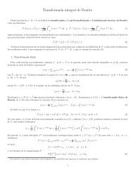
2 Introductionapical dendritessomarecordingelectrodebasal dendritesmembrane potential, mV+35 mVspike40 ms-60 mVtime, mssynapse0.1 mmaxonFigure 1.1: Two interconnected cortical pyramidal neurons (hand drawing) and in vitrorecorded spike.1.1.1 What is a spike?A typical neuron receives inputs from more than 10, 000 other neurons through the contactson its dendritic tree called synapses; see Fig. 1.1. The inputs produce electricaltransmembrane currents that change the membrane potential of the neuron. Synapticcurrents produce changes, called post-synaptic potentials (PSPs). Small currents producesmall PSPs; larger currents produce significant PSPs that could be amplified bythe voltage-sensitive channels embedded in neuronal membrane and lead to the generationof an action potential or spike – an abrupt and transient change of membranevoltage that propagates to other neurons via a long protrusion called an axon.Such spikes are the main means of communication between neurons. In general,neurons do not fire on their own, they do it as a result of the incoming spikes from otherneurons. One of the most fundamental question of neuroscience is what exactly makesneurons fire? What is it in the incoming pulses that elicits a response in one neuronbut not in another one? Why could two neurons have different responses to exactlythe same input and identical responses to completely different inputs? To answerthese questions, we need to understand the dynamics of spike-generation mechanismsof neurons.Most introductory neuroscience books describe neurons as integrators with a threshold:Neurons sum up incoming PSPs and “compare” the integrated PSP with a certainvoltage value, called firing threshold. If it is below the threshold, the neuron remainsquiescent; when it is above the threshold, the neuron fires an all-or-none spike, as inFig. 1.3, and resets its membrane potential. To add theoretical plausibility to thisargument, the books refer to the Hodgkin-Huxley model of spike-generation in squid

Introduction 3Figure 1.2: What makes a neuron fire?giant axons, which we study in the next chapter. The irony is that the Hodgkin-Huxleymodel does not have a well-defined threshold, it does not fire all-or-none spikes, andit is not an integrator, but a resonator, i.e., it prefers inputs having certain frequenciesthat resonate with the frequency of subthreshold oscillations of the neuron. Weconsider these and other properties in detail in this book.1.1.2 Where is the threshold?Much effort has been spent trying to determine experimentally the firing thresholdsof neurons. Here, we challenge the classical view of a threshold. Let us consider twotypical experiments, depicted in Fig. 1.4, that are designed to measure the threshold.On the left, we shock a cortical neuron, i.e., we inject brief but strong pulses of currentof various amplitudes to depolarize the membrane potential to various values. Is therea clear-cut voltage value, as in Fig. 1.3, above which the neuron fires but below whichno spikes occur? If you find one, let the author know! In Fig. 1.4b we inject long butweak pulses of current of various amplitudes, which result in slow depolarization anda spike. The firing threshold, if it exists, must be somewhere in the shaded region, butwhere? Where does the slow depolarization end and the spike start? Is it meaningfulto talk about firing thresholds at all?all-or-nonespikesthresholdrestingno spikeFigure 1.3: The concept of a firing threshold.

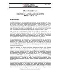
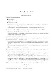
4 Introduction(a)spikes(b)spikes cutthreshold?-40 mVsubthreshold response1 msinjected pulses of current20 mVinjected pulses of current15 msFigure 1.4: Where is the firing threshold? Shown are in vitro recordings of two layer 5pyramidal neurons of rat. Notice the difference of voltage and time scales.(a)(b)20 mV20 mV5 ms100 ms-60 mVFigure 1.5: Where is the rheobase, i.e., the minimal current that fires the cell? (a) invitro recordings of pyramidal neuron of layer 2/3 of rat’s visual cortex show increasinglatencies as the amplitude of the injected current decreases. (b) Simulation of theI Na,p +I K -model shows spikes of graded amplitude.Perhaps, we should measure current thresholds instead of voltage thresholds? Thecurrent threshold, i.e., the minimal amplitude of injected current of infinite durationneeded to fire a neuron, is called rheobase. In Fig. 1.5 we decrease the amplitudesof injected pulses of current to find the minimal one that still elicits a spike or themaximal one that does not. In Fig. 1.5a, progressively weaker pulses result in longerlatencies to the first spike. Eventually the neuron does not fire because the latency islonger than the duration of the pulse, which is 1 second in the figure. Did we reallymeasure the neuronal rheobase? What if we waited a bit longer? How long is longenough? In Fig. 1.5b the latencies do not grow but the spike amplitudes decrease untilthe spikes do not look like spikes at all. To determine the current threshold, we needto draw the line and separate spike responses from “subthreshold” ones. How can wedo that if the spikes are not all-or-none? Is the response denoted by the dashed line aspike?Risking adding more confusion to the notion of a threshold, consider the following:If excitatory inputs depolarize the membrane potential, i.e., bring it closer to the “firingthreshold”, and inhibitory inputs hyperpolarize the potential and move it away from

Introduction 510 ms10 mV-45 mV0 pA-100 pAFigure 1.6: In vitro recording of rebound spikes ofrats brainstem mesV neuron in response to a briefhyperpolarizing pulse of current.10ms5msnon-resonant burst10msresonant burst15msnon-resonant burstinhibitory burstFigure 1.7: Resonant response of the mesencephalic V neuron of rat brainstem to pulsesof injected current having 10 ms period (in vitro).the threshold, then how can the neuron in Fig. 1.6 fire in response to the inhibitoryinput? This phenomenon is also observed in the Hodgkin-Huxley model, and it iscalled anodal break excitation, rebound spike, or post-inhibitory spike. Many biologistssay that rebound responses are due to the activation and inactivation of certain slowcurrents, which bring the membrane potential over the threshold, or equivalently, lowerthe threshold upon release from the hyperpolarization – a phenomenon called a lowthresholdspike in thalamocortical neurons. The problem with this explanation is thatneither the Hodgkin-Huxley model nor the neuron in the figure have these currents,and even if they did, the hyperpolarization is too short and too weak to affect thecurrents.Another interesting phenomenon is depicted in Fig. 1.7. The neuron is stimulatedwith brief pulses of current mimicking an incoming burst of three spikes. When thestimulation frequency is high (5 ms period), presumably reflecting a strong input,the neuron does not fire at all. However, stimulation with a lower frequency (10ms period) that resonates with the frequency of subthreshold oscillation of the neuronevokes a spike response, regardless of whether the stimulation is excitatory or inhibitory.Stimulation with even lower frequency (15 ms period) cannot elicit spike response again.Thus, the neuron is sensitive only to the inputs having resonant frequency. The samepulses applied to a cortical pyramidal neuron evoke a response only in the first case(small period), but not in the other cases.

6 Introduction1.1.3 Why are neurons different and why do we care?Why would two neurons respond completely differently to the same input? A biologistwould say that the response of a neuron depends on many factors, such as the typeof voltage- and Ca 2+ -gated channels expressed by the neuron, the morphology of itsdendritic tree, the location of the input, etc. These factors are indeed important, butthey do not determine the neuronal response per se. They rather determine the rulesthat govern dynamics of the neuron. Different conductances and currents can result inthe same rules and hence in the same responses, and conversely, similar currents canresult in different rules and in different responses. The currents define what kind of adynamical system the neuron is.We study ionic transmembrane currents in the next chapter. In subsequent chapterswe investigate how the type of currents determine neuronal dynamics. We divide allcurrents into two major classes: amplifying and resonant, with persistent Na + currentI Na,p and persistent K + current I K being the typical examples of the former and thelatter. Since there are tens of known currents, purely combinatorial argument impliesthat there are millions of different electrophysiological mechanisms of spike generation.We will show later that any such mechanism must have at least one amplifying and oneresonant current. Some mechanisms, called minimal in this book, have precisely oneresonant and one amplifying current. They provide an invaluable tool in classifyingand understanding the electrophysiology of spike-generation.Many illustrations in this book are based on simulations of the reduced I Na,p + I K -model, which consists of fast persistent Na + (amplifying) current and slower persistentK + (resonant) current. It is equivalent to the famous and widely used Morris-LecarI Ca + I K -model (Morris and Lecar 1981). We show that the model exhibits quite differentdynamics depending on the values of the parameters, e.g., the half-activationvoltage of the K + current: In one case, it can fire in a narrow frequency range, exhibitco-existence of resting and spiking states, damped subthreshold oscillations of membranepotential, etc. In another case, it can fire in a wide frequency range and show noco-existence of resting and spiking and no subthreshold oscillations. Thus, seeminglyinessential differences in parameter values could result in drastically distinct behaviors.1.1.4 Building modelsTo build a good model of a neuron, electrophysiologists apply different pharmacologicalblockers to tease out the currents that the neuron has. Then, they apply differentstimulation protocols to measure the kinetic parameters of the currents, such as theBoltzmann activation function, time constants, maximal conductances, etc. We considerall these functions in the next chapter. Then, they create a Hodgkin-Huxley-typemodel and simulate it using NEURON, GENESIS, XPP environments or just plainMATLAB (the first two are invaluable tools for simulating realistic dendritic structures).The problem is that the parameters are measured in different neurons and then puttogether into a single model. As an illustration, consider two neurons having the same

Introduction 7Figure 1.8: Neurons are dynamical systems.currents, say I Na,p and I K , and exhibiting excitable behavior; that is, both neurons arequiescent but can fire a spike in response to a stimulation. Suppose the second neuronhas stronger I Na,p , which is balanced by stronger I K . If we measure Na + conductanceusing the first neuron and K + conductance using the second neuron, the resultingI Na,p + I K -model would have an excess of K + current and probably not be able to firespikes at all. Conversely, if we measure Na + and K + conductances using the secondand then the first neuron, respectively, the model would have too much Na + currentand probably exhibit sustained pacemaking activity. In any case, the model fails toreproduce the excitable behavior of the neurons whose parameters we measured.Some of the parameters cannot be measured at all, so many arbitrary choices aremade via a process called “fine-tuning”. Navigating in the dark, possibly with the helpof some biological intuition, the researcher modifies parameters, compares simulationswith experiment, and repeats this trial-and-error procedure until he or she is satisfiedwith the results. Since seemingly similar values of parameters can result in drasticallydifferent behaviors, and quite different parameters can result in seemingly similar behaviors,how do we know that the resulting model is correct? How do we know that itsbehavior is equivalent to that of the neuron we want to study? And what is equivalentin this case? Now, the reader is primed to consider dynamical systems.1.2 Dynamical SystemsIn the next chapter we introduce the Hodgkin-Huxley formalism to describe neuronaldynamics in terms of activation and inactivation of voltage-gated conductances. Animportant consequence of the Hodgkin-Huxley studies is that neurons are dynamicalsystems, so they should be studied as such. Below we mention some of the important

8 Introductionconcepts of dynamical systems theory. The reader does not have to follow all the detailsof this section because the concepts are explained in a greater detail in subsequentchapters.A dynamical system consists of a set of variables that describe its state and alaw that describes the evolution of the state variables with time, i.e., how the stateof the system in the next moment of time depends on the input and its state in theprevious moment of time. The Hodgkin-Huxley model is a four-dimensional dynamicalsystem because its state is determined uniquely by the membrane potential, V , and socalled gating variables n, m and h for persistent K + and transient Na + currents. Theevolution law is given by a four-dimensional system of ordinary differential equations.Typically, all variables describing neuronal dynamics can be classified into fourclasses, according to their function and the time scale:1. Membrane potential.2. Excitation variables, such as activation of Na + current. This variables are responsiblefor the upstroke of the spike.3. Recovery variables, such as inactivation of Na + current and activation of fast K +current. This variables are responsible for the repolarization (downstroke) of thespike.4. Adaptation variables, such as activation of slow voltage- or Ca 2+ -dependent currents.This variables build up during prolonged spiking and can affect excitabilityon the long run.The Hodgkin-Huxley model does not have variables of the fourth type, but manyneuronal models do, especially those exhibiting bursting dynamics.1.2.1 Phase portraitsThe power of the dynamical systems approach to neuroscience, as well as to manyother sciences, is that we can tell something, or many things, about a system withouteven knowing all the details that govern the system evolution. We do not even useequations to do that! Some may even wonder why we call it a mathematical theory.As a start, let us consider a quiescent neuron whose membrane potential is resting.From the dynamical systems point of view, there are no changes of the statevariables of such a neuron, hence it is at an equilibrium point. All the inward currentsthat depolarize the neuron are balanced, or equilibrated, by the outward currents thathyperpolarize it. If the neuron remains quiescent despite small disturbances and membranenoise, as in Fig. 1.9a, top, then we conclude that the equilibrium is stable. Isn’tit amazing that we can make such a conclusion without knowing the equations thatdescribe the neuron’s dynamics? We do not even know the number of variables neededto describe the neuron; it could be infinite, for all we care.

Introduction 9K + activation gate, n membrane potential, V(t)(a) resting (b) excitable (c) periodic spikingPSPstimulusequilibriummembrane potential, Vtime, tPSPA BstimuliPSPA BspikespikeperiodicorbitFigure 1.9: Resting, excitable, and periodic spiking activity correspond to a stableequilibrium (a and b) or limit cycle (c), respectively.In this book we introduce the notions of equilibria, stability, threshold, and attractiondomains using one- and two-dimensional dynamical systems, e.g., the I Na,p +I K -model with instantaneous Na + kinetics. Its state is described by the membrane potential,V , and the activation variable, n, of the persistent K + current, so it is atwo-dimensional vector (V, n). Instantaneous activation of Na + current is a functionof V , so it does not result in a separate variable of the model. The evolution of themodel is a trajectory (V (t), n(t)) on the V × n-plane. Depending on the initial point,the system can have many trajectories, such as those depicted in Fig. 1.9a, bottom.Time is not present explicitly in the figure, but units of time may be thought of asplotted along each trajectory. All of the trajectories in the figure are attracted to thestable equilibrium denoted by the black dot, called an attractor. The overall qualitativedescription of dynamics can be obtained through the study of the phase portrait of thesystem, which depicts certain special trajectories (equilibria, separatrices, limit cycles)that determine the topological behavior of all the other trajectories in the phase space.Probably 50 % of illustrations in this book are phase portraits.A fundamental property of neurons is excitability, illustrated in Fig. 1.9b. Theneuron is resting, i.e., its phase portrait has a stable equilibrium. Small perturbations,such as A, result in small excursions from the equilibrium, denoted as PSP (postsynapticpotential). In contrast, larger perturbations, such as B, are amplified bythe neuronal intrinsic dynamics and result in the spike response. To understand thedynamic mechanism of such amplification, we need to consider the geometry of thephase portrait near the equilibrium, i.e., in the region where the decision to fire or notto fire is made.If we inject a sufficiently strong current into the neuron, we bring it to a pacemakingmode, so that it exhibits periodic spiking activity, as in Fig. 1.9c. From the dynamical

10 Introductionspikingmoderesting modeFigure 1.10: Rhythmic transitions between resting and spiking modes result in burstingbehavior.layer 5 pyramidal cellbrainstem mesV celltransition20 mVtransition-60 mV-50 mV200 pA3000 pA0 pA500 ms0 pA500 msFigure 1.11: As the magnitude of the injected current slowly increases, the neuronsbifurcate from resting (equilibrium) to tonic spiking (limit cycle) modes.systems point of view, the state of such a neuron has a stable limit cycle, also knownas a periodic orbit. The electrophysiological details of the neuron, i.e., the numberand the type of currents it has, their kinetics, etc., determine only the location, theshape and the period of the limit cycle. As long as the limit cycle exists, the neuroncan have periodic spiking activity. Of course, equilibria and limit cycles can co-exist,so a neuron can be switched from one mode to another one by a transient input. Thefamous example is the permanent extinguishing of ongoing spiking activity in the squidgiant axon by a brief transient depolarizing pulse of current applied at a proper phase(Guttman et al. 1980) — a phenomenon predicted by John Rinzel (1978) purely onthe basis of theoretical analysis of the Hodgkin-Huxley model. The transition betweenresting and spiking modes could be triggered by intrinsic slow conductances, resultingin the bursting behavior in Fig. 1.10.1.2.2 BifurcationsNow suppose that the magnitude of the injected current is a parameter that we cancontrol, e.g., we can ramp it up as in Fig. 1.11. Each cell in the figure is quiescentat the beginning of the ramps, so its phase portrait has a stable equilibrium and it

Introduction 11may look like the one in Fig. 1.9a or b. Then it starts to fire tonic spikes, so its phaseportrait has a limit cycle attractor and it may look like the one in Fig. 1.9c, with whitecircle denoting an unstable resting equilibrium. Apparently, there is some intermediatelevel of injected current that corresponds to the transition from resting to sustainedspiking, i.e., from the phase portrait in Fig. 1.9b to Fig. 1.9c. What does the transitionlook like?From dynamical systems point of view, the transition corresponds to a bifurcationof neuron dynamics, i.e., a qualitative change of phase portrait of the system. Forexample, there is no bifurcation going from phase portrait in Fig. 1.9a to that inFig. 1.9b, since both have one globally stable equilibrium; the difference in behavior isquantitative but not qualitative. In contrast, there is a bifurcation going from Fig. 1.9bto Fig. 1.9c since the equilibrium is no longer stable and another attractor, limit cycle,appeared. The neuron is not excitable in Fig. 1.9a but it is in Fig. 1.9b simply becausethe former phase portrait is far away from the bifurcation and the latter is near.In general, neurons are excitable because they are near bifurcations from resting tospiking activity, so the type of the bifurcation determines the excitable properties of theneuron. Of course, the type depends on the neuron’s electrophysiology. An amazingobservation is that there could be millions of different electrophysiological mechanismsof excitability and spiking, but there are only 4, yes four, different types of bifurcationsof equilibrium that a system can undergo without any additional constraints, suchas symmetry. Thus, considering these four bifurcations in a general setup we canunderstand excitable properties of many models, even those that have not been inventedyet. What is even more amazing, we can understand excitable properties of neuronswhose currents are not measured and whose models are not known, provided thatwe can identify experimentally which of the four bifurcations the resting state of theneuron undergoes.The four bifurcations are summarized in Fig. 1.12, which plots the phase portraitbefore (left), at (center), and after (right) a particular bifurcation occurs. Mathematiciansrefer to these bifurcations as being of co-dimension-1 because we need to vary onlyone parameter, e.g., the magnitude of the injected dc-current I, to observe the bifurcationsreliably in simulations or experiments. There are many more co-dimension-2,3, etc., bifurcation, but they need special conditions to be observed. We discuss theselater in Chap. 6.Let us consider the four bifurcation and their phase portraits in the figure. Thehorizontal and vertical axes are the membrane potential with instantaneous activationvariable and a recovery variable, respectively. At this stage, the reader is not requiredto fully understand the intricacies of the phase portraits in the figure, since they willbe explained systematically in later chapters.• Saddle-node bifurcation. As the magnitude of the injected current or any otherbifurcation parameter changes, a stable equilibrium corresponding to the restingstate (black circle marked “node” in Fig. 1.12a) is approached by an unstableequilibrium (white circle marked “saddle”), they coalesce and annihilate eachother, as in Fig. 1.12a, middle. Since the resting state no longer exists, the

12 Introduction(a)spikinglimitcyclerecoverypotentialnodesaddlesaddle-nodesaddle-node bifurcation(b)invariantcirclenode saddle saddle-nodesaddle-node on invariant circle (SNIC) bifurcation(c)spikinglimitcycle attractorunstablesubcritical Andronov-Hopf bifurcation(d)supercritical Andronov-Hopf bifurcationFigure 1.12: Four generic (co-dimension-1) bifurcations of an equilibrium state leadingto the transition from resting to periodic spiking behavior in neurons.

Introduction 13trajectory describing the evolution of the system jumps to the limit cycle attractorindicating that the neuron starts to fire tonic spikes. Notice that the limit cycle,or some other attractor, must co-exist with the resting state in order for thetransition resting → spiking to occur.• Saddle-node on invariant circle bifurcation is similar to the saddle-node bifurcationabove with the exception that there is an invariant circle at the moment ofbifurcation, which then becomes a limit cycle attractor, as in Fig. 1.12b.• Subcritical Andronov-Hopf bifurcation. A small unstable limit cycle shrinks toa stable equilibrium and makes it lose stability, as in Fig. 1.12c. Because ofinstabilities, the trajectory diverges from the equilibrium and approaches a largeamplitudespiking limit cycle or some other attractor.• Supercritical Andronov-Hopf bifurcation. The stable equilibrium loses stabilityand gives birth to a small-amplitude limit cycle attractor, as in Fig. 1.12d. Asthe magnitude of the injected current increases, the amplitude of the limit cycleincreases and it becomes full-size spiking limit cycle.Notice that there is a co-existence of resting and spiking states in the case of saddle-nodeand subcritical Andronov-Hopf bifurcations, whereas there is not in the other two cases.Such a co-existence reveals itself via a hysteresis behavior when the injected currentincreases and then decreases past the bifurcation value, because the transitions “resting→ spiking” and “spiking → resting” occur at different values of the current. In addition,brief stimuli applied at the appropriate times can switch the activity from spiking toresting and back. There are also spontaneous noise-induced transitions between thetwo modes resulting in the stuttering spiking, as e.g. exhibited by the so called fastspiking (FS) cortical interneurons when they are kept close to the bifurcation (Tatenoet al. 2004). Some bistable neurons have a slow adaptation current that activatesduring the spiking mode and impedes spiking, often resulting in bursting activity.Systems undergoing Andronov-Hopf bifurcations, whether subcritical or supercritical,exhibit damped oscillations of membrane potential, whereas systems near saddlenodebifurcations, whether on or off an invariant circle, do not. The existence ofsmall amplitude oscillations creates the possibility of resonance to the frequency of theincoming pulses, as in Fig. 1.7, and other interesting features.We refer to neurons with damped subthreshold oscillations as resonators and tothose that do not have this property as integrators. We refer to the neurons that exhibitthe co-existence of resting and spiking states, at least near the transition from resting tospiking, as bistable, and to those that do not exhibit the bistability as monostable. Thefour bifurcations in Fig. 1.12 are uniquely defined by these two features. For example,a bistable resonator is a neuron undergoing subcritical Andronov-Hopf bifurcation,and a monostable integrator is a neuron undergoing saddle-node on invariant circlebifurcation; see table in Fig. 1.13. Cortical fast spiking (FS) and regular spiking(RS) neurons, studied in Chap. 8, are typical examples of the former and the latter,respectively.

14 Introductionco-existence of resting and spiking statesYES(bistable)NO(monostable)subthreshold oscillationsNO(integrator)YES(resonator)saddle-nodesubcriticalAndronov-Hopfsaddle-node oninvariant circlesupercriticalAndronov-HopfFigure 1.13: Classification of neurons intomonostable/bistable integrators/resonatorsaccording to the bifurcation of the restingstate in Fig. 1.12.asymptotic firing frequency, Hz40302010Class 1 excitabilityF-I curve00 100 200 300injected dc-current, I (pA)asymptotic firing frequency, Hz25020015010050Class 2 excitabilityF-I curve00 500 1000 1500injected dc-current, I (pA)Figure 1.14: Frequency-current (F-I) curves of cortical pyramidal neuron and brainstemmesV neuron from Fig. 7.3. These are the same neurons used in the ramp experimentin Fig. 1.11.1.2.3 Hodgkin classificationHodgkin (1948) was the first to study bifurcations in neuronal dynamics, years beforethe mathematical theory of bifurcations was developed. He stimulated squid axonswith pulses of various amplitudes and identified three classes of responses:• Class 1 neural excitability. Action potentials can be generated with arbitrarilylow frequency, depending on the strength of the applied current.• Class 2 neural excitability. Action potentials are generated in a certainfrequency band that is relatively insensitive to changes in the strength of theapplied current.• Class 3 neural excitability. A single action potential is generated in responseto a pulse of current. Repetitive (tonic) spiking can be generated only forextremely strong injected currents or not at all.The qualitative distinction between the classes is that the frequency-current relation(the F-I curve in Fig. 1.14) starts from zero and continuously increases for Class 1

Introduction 15neurons, is discontinuous for Class 2 neurons, and is not defined at all for Class 3neurons.Obviously, neurons belonging to different classes have different neuro-computationalproperties: Class 1 neurons, which include cortical excitatory pyramidal neurons, cansmoothly encode the strength of the input into the output firing frequency, as inFig. 1.11, left. In contrast, Class 2 neurons, such as fast-spiking (FS) cortical inhibitoryinterneurons, cannot do that; instead, they fire in a relatively narrow frequency band,as in Fig. 1.11, right. Class 3 neurons cannot exhibit sustained spiking activity, soHodgkin regarded them as “sick” or “unhealthy”. There are other distinctions betweenthe classes, which we discuss later.Different classes of excitability occur because neurons have different bifurcations ofresting and spiking states – a phenomenon first explained by Rinzel and Ermentrout(1989). If ramps of current are injected to measure the F-I curves, then Class 1 excitabilityoccurs when the neuron undergoes the saddle-node bifurcation on invariantcircle depicted in Fig. 1.12b. Indeed, the period of the limit cycle attractor is infiniteat the bifurcation point, and then it decreases as the bifurcation parameter – say, theinjected current – increases. The other three bifurcations result in Class 2 excitability.Indeed, the limit cycle attractor exists and has a finite period when the resting statein Fig. 1.12 undergoes a subcritical Andronov-Hopf bifurcation, so emerging spikinghas a non-zero frequency. The period of the small limit cycle attractor appearing viasupercritical Andronov-Hopf bifurcation is also finite, so the frequency of oscillationsis non-zero, but their amplitudes are small. In contrast to the common and erroneousfolklore, the saddle-node bifurcation (off limit cycle) also results in Class 2 excitabilitybecause the limit cycle has a finite period at the bifurcation. There is a considerablelatency (delay) to the first spike in this case, but the subsequent spiking has non-zerofrequency. Thus, the simple scheme “Class 1 = saddle-node, Class 2 = Hopf” thatpermeates many publications is incorrect.When pulses of current are used to measure the F-I curve, as in Hodgkin’s experiments,the firing frequency depends on other factors, and not only the type of thebifurcation of the resting state. In particular, low-frequency firing can be observed insystems near Andronov-Hopf bifurcations, as we show in Chap. 7. To avoid possibleconfusion, we define the class of excitability based only on slow ramp experiments.Hodgkin’s classification has an important historical value but it is of little use forthe dynamic description of a neuron, since naming a class of excitability of a neurondoes not tell much about the bifurcations of the resting state. Indeed, it only says thatsaddle-node on invariant circle bifurcation (Class 1) is different from the other threebifurcations (Class 2), and only when ramps are injected. Instead, dividing neurons intointegrators and resonators with bistable or monostable activity is more informative, sowe adopt the classification in Fig. 1.13 in this book. In this classification, Class 1 neuronis a monostable integrator, whereas Class 2 neuron could be a bistable integrator or aresonator.

16 Introduction1.2.4 Neuro-computational propertiesUsing the same arrangement as in Fig. 1.13, we depict typical geometry of phaseportraits near the four bifurcations in Fig. 1.15. Let us use the portraits to explain whathappens “near the threshold”, i.e., near the place where the decision to fire or not ismade. To simplify our geometrical analysis we assume here that neurons receive shockinputs, i.e., brief but strong pulses of current that do not change the phase portraitsbut only push or reset the state of the neuron into various regions of the phase space.We consider these and other cases in detail in Chap. 7.The horizontal axis in each plot in Fig. 1.15 corresponds to the membrane potentialV with instantaneous Na + current, and the vertical axis corresponds to a recovery variable,say activation of K + current. Black circles denote stable equilibria correspondingto the neuronal resting state. Spiking limit cycle attractors correspond to sustainedspiking states, which exist in the two cases depicted in the left half of the figure correspondingto the bistable dynamics. The limit cycles are surrounded by the shadedregions — their attraction domains. The white region is the attraction domain of theequilibrium. To initiate spiking, the external input should push the state of the systeminto the shaded region, and to extinguish spiking, the input should push the state backinto the white region.There are no limit cycles in the two cases depicted in the right half of the figure,so the entire phase space is the attraction domain of the stable equilibrium, and thedynamics are monostable. However, if the trajectory starts in the shaded region, itmakes a large-amplitude rotation before returning to the equilibrium — a transientspike. Apparently, to elicit such a spike, the input should push the state of the systeminto the shaded region.Now let us contrast the upper and lower halves of the figure corresponding tointegrators and resonators, respectively. We distinguish these two modes of operationbased on the existence of subthreshold oscillations near the equilibrium.First, let us show that inhibition impedes spiking in integrators, but can promote itin resonators. In the integrator case, the shaded region is in the depolarized voltagerange, i.e., to the right of the equilibrium. Excitatory inputs push the state of thesystem toward the shaded region, while inhibitory inputs push it away. In the case ofresonators, both excitation and inhibition push the state toward the shaded region, becausethe region wraps around the equilibrium and can be reached along any direction.This explains the rebound spiking phenomenon depicted in Fig. 1.6.Integrators have all-or-none spikes while resonators may not. Indeed, any trajectorystarting in the shaded region in the upper half of the figure has to rotate aroundthe white circle at the top corresponding to an unstable equilibrium. Moreover, thestate of the system is quickly attracted to the spiking trajectory and moves along thetrajectory thereby generating a stereotypical spike. A resonator neuron can also firelarge-amplitude spikes when its state is pushed to or beyond the trajectory denoted“spike”. Such neurons generate subthreshold responses when the state slides along

Introduction 17saddle-node bifurcationsaddle-node on invariant circle bifurcationrecoverypotentialspikingthresholdlimitcycle attractorspikingtrajectorythresholdinhexc12subcritical Andronov-Hopf bifurcationsupercritical Andronov-Hopf bifurcationspiking limitcycle attractorhalf-amplitudespikespikehalf-amplitudespikePSPspike1inhPSPexc23Figure 1.15: The geometry of phase portraits of excitable systems near 4 bifurcationscan explain many neuro-computational properties (see Sect. 1.2.4 for detail).the smaller trajectory denoted “PSP”; they can also generate spikes of an intermediateamplitude when the state is pushed between the “PSP” and “spike” trajectories, whichexplains the partial-amplitude spiking in Fig. 1.5 or in the squid axon in Fig. 7.26. Theset of initial conditions corresponding to such spiking is quite small, so typical spikeshave large amplitudes and partial spikes are rare.Integrators have well-defined thresholds while resonators may not. The white circlesnear the resting states of integrators in Fig. 1.15 are called saddles. They are stablealong the vertical direction and unstable along the horizontal direction. The two trajectoriesthat lead to the saddle along the vertical direction are called separatrices becausethey separate the phase space into two regions, in this case into white and shaded. Theseparatrices play the role of thresholds since only those perturbations that push thestate of the system beyond the separatrices result in a spike. The closer is the state of

18 IntroductionspikeFigure 1.16: Phase portrait of a system near aBogdanov-Takens bifurcation that corresponds tothe transition from integrator to resonator mode.the system to the separatrices, the longer it takes to converge and then diverge fromthe saddle, resulting in a long latency to the spike. Notice that the threshold is not apoint but a tilted curve that spans a range of voltage values.Resonators have a well-defined threshold in the case of subcritical Andronov-Hopfbifurcation: it is the small unstable limit cycle that separates the attraction domainsof stable equilibrium and spiking limit cycle. Trajectories inside the small cycle spiraltoward the stable equilibrium, while trajectories outside the cycle spiral away andeventually lead to sustained spiking activity. When a neuronal model is far from thesubcritical Andronov-Hopf bifurcation, its phase portrait may look similar to the onecorresponding to the supercritical Andronov-Hopf bifurcation. The narrow shadedband in the figure is not a threshold manifold but a fuzzy threshold set called “quasithreshold”by FitzHugh (1955). Many resonators, including the Hodgkin-Huxley modelhave quasi-thresholds. The width of the quasi-threshold in the Hodgkin-Huxley modelis so narrow, that it may be assumed to be just a curve for all practical reasons.Integrators integrate, resonators resonate. Now consider inputs consisting of multiplepulses, e.g., a burst of spikes. Integrators prefer high-frequency inputs; the higherthe frequency, the sooner they fire. Indeed, the first spike of such an input, marked“1” in the top-right phase portrait in Fig. 1.15, increases the membrane potential andshifts the state to the right toward the threshold. Since the state of the system isstill in the white area, it slowly converges back to the stable equilibrium. To crossthe threshold manifold, the second pulse must arrive shortly after the first one. Thereaction of a resonator to a pair of pulses is quite different. The first pulse initiates adamped subthreshold oscillation of the membrane potential, which looks like a spiralin the bottom-right phase portrait in Fig. 1.15. The effect of the second pulse dependson its timing. If it arrives after the trajectory makes half a rotation, marked as “2”in the figure, it cancels the effect of the first pulse. If it arrives after the trajectorymakes a full rotation, marked “3” in the figure, it adds to the first pulse and eitherincreases the amplitude of subthreshold oscillation or evokes a spike response. Thus,the response of the resonator neuron depends on the frequency content of the input,as in Fig. 1.7.Integrators and resonators constitute two major modes of activity of neurons. Mostcortical pyramidal neurons, including the regular spiking (RS), intrinsically bursting

Introduction 19(IB), and chattering (CH) types considered in Chap. 8, are integrators. So are thalamocorticalneurons in the relay mode of firing and neostriatal spiny projection neurons.Most cortical inhibitory interneurons, including the fast spiking type, are resonators.So are brainstem mesencephalic V neurons and stellate neurons of the entorhinal cortex.Some cortical pyramidal neurons and low-threshold spiking (LTS) interneurons can beat the border of transition between integrator and resonator modes. Such a transitioncorresponds to another bifurcation, which has co-dimension-2, and hence it is less likelyto be encountered experimentally. We consider this and other uncommon bifurcationsin detail later. The phase portrait near the bifurcation is depicted in Fig. 1.16 and it isa good exercise for the reader to explain why such a system has damped oscillations andpost-inhibitory responses yet a well-defined threshold, all-or-none spikes with possiblylong latencies.Of course, figures 1.15 and 1.16 cannot encompass all the richness of neuronalbehavior, otherwise this book would be only 19-pages long 1 . Many aspects of neuronaldynamics depend on other bifurcations, e.g., those corresponding to appearance anddisappearance of spiking limit cycles. These bifurcations describe the transitions fromspiking to resting, and they are especially important when we consider bursting activity.In addition, we need to take into account the relative geometry of equilibria, limitcycles, and other relevant trajectories, and how they depend on the parameters of thesystem, such as maximal conductances, activation time constants, etc. We explore allthese issues systematically in subsequent chapters.In Chap. 2 we review some of the most fundamental concepts of neuron electrophysiology,culminating with the Hodgkin-Huxley model. This chapter is aimed atmathematicians learning neuroscience. In Chapters 3 and 4 we use one- and twodimensionalneuronal models, respectively, to review some of the most fundamentalconcepts of dynamical systems, such as equilibria, limit cycles, stability, attractiondomain, nullclines, phase portrait, bifurcation, etc. The material in these chapters,aimed at biologists learning the language of dynamical systems, is presented with theemphasis on geometrical rather than mathematical intuition. In fact, the spirit of theentire book is to explain concepts using pictures, not equations. Chap. 5 exploresphase portraits of various conductance-based models and the relations between ioniccurrents and dynamic behavior. In Chap. 6 we use the I Na,p +I K -model to systematicallyintroduce the geometric bifurcation theory. Chap. 7, probably the most importantchapter of the book, applies the theory to explain many computational properties ofneurons. In fact, all the material in the previous chapters is given so that the readercan understand this chapter. In Chap. 8 we use a simple phenomenological model tosimulate many cortical and thalamic neurons. This chapter contains probably the mostcomprehensive up to date review of various firing patterns exhibited by mammalianneurons. In Chap. 9 we introduce the electrophysiological and topological classificationof bursting dynamics, as well as some useful methods to study the bursters. Finally,the last and the most mathematically advanced chapter of the book, Chap. 10, deals1 This book is actually quite short; Most of the space is taken by figures, exercises, and solutions.

20 Introductionwith coupled neurons. There we show how the details of spike-generation mechanismof neurons affect their collective properties, such as synchronization.1.2.5 Building models (revisited)To have a good model of a neuron, it is not enough to put the right kind of currents togetherand tune the parameters so that the model can fire spikes. It is not even enoughto reproduce the right input resistance, rheobase, and firing frequencies. The modelhas to reproduce all the neuro-computational features of the neuron, starting withthe co-existence of resting and spiking states, spike latencies, subthreshold oscillations,rebound spikes, etc.A good way to start is to determine what kind of bifurcations the neuron underconsideration undergoes and how the bifurcations depend on neuromodulators andpharmacological blockers. Instead of or in addition to measuring neuronal responsesto get the kinetic parameters, we need to measure them to get the right bifurcationbehavior. Only in this case we can be sure that the behavior of the model is equivalentto that of the neuron, even if we omitted a current or guessed some of the parametersincorrectly.Implementation of this research program is still a pipe dream. The people whounderstand the mathematical aspects of neuron dynamics, those who see beyond conductancesand currents, those people do not usually have the opportunity to do experiments.Conversely, those who study neurons in vitro or in vivo on a daily basis,those who see spiking, bursting, oscillations, those who can manipulate the experimentalsetup to test practically any aspect of neuronal activity, those people do notusually see the value of studying phase portraits, bifurcations, and nonlinear dynamicsin general. One of the goals of this book is to change this state and bring these twogroups of people closer together.

Introduction 21Review of Important Concepts• Neurons are dynamical systems.• Resting state of neurons corresponds to a stable equilibrium, tonicspiking state corresponds to a limit cycle attractor.• Neurons are excitable because the equilibrium is near a bifurcation.• There are many ionic mechanisms of spike-generation, but only fourgeneric bifurcations of equilibria.• These bifurcations divide neurons into four categories: integratorsor resonators, monostable or bistable.• Analyses of phase portraits at bifurcations explain why some neuronshave well-defined thresholds, all-or-none spikes, post-inhibitoryspikes, frequency preference, hysteresis, etc., while others do not.• These features, and not ionic currents per se, determine the neuronalresponses, i.e., the kind of computations neurons do.• A good neuronal model must reproduce not only electrophysiologybut also the bifurcation dynamics of neurons.Bibliographical NotesRichard FitzHugh at the National Institutes of Health (NIH) pioneered the phase planeanalysis of neuronal models with the view to understand their neuro-computationalproperties. He was the first to analyze the Hodgkin-Huxley model (FitzHugh 1955;years before they received the Nobel prize) and to prove that it has neither thresholdnor all-or-none spikes. FitzHugh (1961) introduced a simplified model of excitabilityand showed that one can get the right kind of neuronal dynamics in models lackingconductances and currents. Nagumo et al. (1962) designed a corresponding tunneldiode circuit, so the model is called the FitzHugh-Nagumo oscillator. Chapter 8 dealswith such simplified models.FitzHugh research program was further developed by John Rinzel and G. BardErmentrout. In their 1989 seminal paper, Rinzel and Ermentrout revived Hodgkin’sclassification of excitability and pointed out to the connection between the behavior ofneuronal models and the bifurcations they exhibit. (They also refer to the excitabilityas “type I” and “type II”). Unfortunately, many people treat the connection in asimpleminded fashion and incorrectly identify “type I = saddle-node, type II = Hopf”.

22 IntroductionFigure 1.17: John Rinzel in 2004. Incidentally, his T-shirt shows the cover of the firstissue of Journal of Computational Neuroscience, in which the Pinsky-Rinzel (1994)model appeared.Figure 1.18: G. Bard Ermentrout (G. stands for George) with his parrot Junior in1983.

Introduction 23Figure 1.19: Richard FitzHugh in 1984.If only life was so simple!The geometrical analysis of neuronal models was further developed, among others,by Izhikevich (2000), who stressed the integrator and resonator modes of operationand made connections to other neuro-computational properties.The neuroscience and mathematics parts of this book are standard, though manyconnections are new. We point to the literature sources at the end of each chapter.Among many outstanding books on computational neuroscience, we especially recommendSpikes, Decisions, and Actions by Wilson (1999), Biophysics of Computation byKoch (1999), Theoretical Neuroscience by Dayan and Abbott (2001), and Foundationsof Cellular Neurophysiology by Johnston and Wu (1995). The present monographcomplements these excellent books in the sense that it is more ambitious, focused,and thorough in dealing with neurons as dynamical systems. Though the views inthis monograph may be biased by the author’s philosophy and taste, the payoffs inunderstanding neuronal dynamics are immense, provided that the reader has enoughpatience and perseverance to follow the author’s line of thought.NEURON simulation environment is described by Hines (1989) (http://www.neuron.yale.edu),GENESIS environment is described by Bower and Beeman (1995) (http://www.genesis-sim.org),XPP environment is described by Ermentrout (2002). The author of this book usesMATLAB (version 6.5 for Windows), which has become a standard computational toolin science and engineering (MATLAB is registered trademark of The MathWorks, Inc.;see http://www.mathworks.com).

24 Introduction

Chapter 2Electrophysiology of NeuronsIn this chapter we remind the reader of some fundamental concepts of neuronal electrophysiology,which are necessary to understand the rest of the book. We start with ionsand currents, and move quickly toward the dynamics of the Hodgkin-Huxley model.If the reader is already familiar with the Hodgkin-Huxley formalism, this chapter canbe skipped. Our exposition is brief, and it cannot substitute a good introductory neurosciencecourse or reading of such excellent textbooks as Theoretical Neuroscience byDayan and Abbott (2001), Foundations of Cellular Neurophysiology by Johnston andWu (1995), Biophysics of Computation by Koch (1999) or Ion Channels of ExcitableMembranes by Hille (2001).2.1 IonsElectrical activity in neurons is sustained and propagated via ionic currents throughneuron membranes. Most of these transmembrane currents involve four ionic species:sodium (Na + ), potassium (K + ), calcium (Ca 2+ ), and chloride (Cl − ). The first threehave a positive charge (cations) and the fourth has a negative charge (anion). Theconcentrations of these ions are different on the inside and outside of a cell, whichcreates electrochemical gradients — the major driving forces of neural activity. Theextracellular medium has high concentration of Na + and Cl − (salty like seawater) and arelatively high concentration of Ca 2+ . The intracellular medium has high concentrationof K + and negatively charged molecules (denoted by A − ), as we illustrate in Fig. 2.1.The cell membrane has large protein molecules forming channels through whichions (but not A − ) can flow according to their electrochemical gradients. The flow ofNa + and Ca 2+ ions is not significant, at least at rest, but the flow of K + and Cl − ionsis. This, however, does not eliminate the concentration asymmetry due to the followingtwo reasons.• Passive redistribution. The impermeable anions A − attract more K + into the cell(opposites attract) and repel more Cl − out of the cell, thereby creating concentrationgradients.• Active transport. Ions are pumped in and out of the cell via ionic pumps. Forexample, the Na + -K + pump depicted in Fig. 2.1 pumps out three Na + ions for25

26 Electrophysiology of NeuronsInsideNa + (5-15 mM)K + (140 mM)Cl-(4 mM)Ca 2+ (0.1 µ M)A-(147 mM)ActiveTransportNa +Na + Na +PumpK + K +K +A -OutsideK + A - Na + Cl -Na + (145 mM)K + (5 mM)Cl-(110 mM)Ca 2+ (2.5-5 mM)A-(25 mM)Cl -PassiveRedistributionEquilibrium PotentialsNa + 62 log 1455= 90 mV62 log 14515= 61 mVK + 62 log 5140= −90 mVCl − −62 log 1104= −89 mVCa 2+ 31 log 2.510 −4 = 136 mV31 log 510 −4 = 146 mVFigure 2.1: Ion concentrations and Nernst equilibrium potentials (2.1) in a typicalmammalian neuron (modified from Johnston and Wu 1995). A − are membraneimpermeantanions. Temperature T = 37 ◦ C (310 ◦ K).every two K + ions pumped in, thereby maintaining concentration gradients.2.1.1 Nernst potentialThere are two forces that drive each ion species through the membrane channel: concentrationand electric potential gradients. First, the ions diffuse down the concentrationgradient. For example, the K + ions depicted in Fig. 2.2a diffuse out of the cell becauseK + concentration inside is higher than that outside. While exiting the cell, K + ionscarry positive charge with them and leave a net negative charge inside the cell (consistingmostly of impermeable anions A − ), thereby producing the outward current. Thepositive and negative charges accumulate on the opposite sides of the membrane surfacecreating an electric potential gradient across the membrane – transmembrane potentialor membrane voltage. This potential slows down the diffusion of K + , since K + ions areattracted to the negatively charged interior and repelled from the positively chargedexterior of the membrane, as we illustrate in Fig. 2.2b. At some point an equilibriumis achieved: The concentration gradient and the electric potential gradient exert equaland opposite forces that counterbalance each other, and the net cross-membrane currentis zero, as in Fig. 2.2c. The value of such an equilibrium potential depends on theionic species, and it is given by the Nernst equation (Hille 2001)E ion = RTzF ln [Ion] out[Ion] in, (2.1)

Electrophysiology of Neurons 27InsideOutsideInsideOutsideInsideOutsideK + Na + Cl -A - Na +Cl -DiffusionK +Cl - Na +K + A -A -K +K +Cl -A -Na + Na +A - Cl -K +Na +A -K + Na + Na +A -Cl -A -K +Cl -A - Na +A -K +Na +Cl - A - K + Cl -DiffusionDiffusionK + A -K + Cl - K + A - Na + Cl -K +A - K +A -K +Na +A - A -K +K +K +A - K +A - K +Cl -A - K +A - ClA - Electric-ElectricNaPotential+ K + A -KPotential+Na +A - Na +A - K +A -K +Cl -K +A - A - K+Na +Na +K +Cl -A - A -K +Na +A -Cl -Cl -K +Cl -a b cFigure 2.2: Diffusion of K + ions down the concentration gradient though the membrane(a) creates an electric potential force pointing in the opposite direction (b) until thediffusion and electrical forces counter each other (c). The resulting transmembranepotential (2.1) is referred to as the Nernst equilibrium potential for K + .where [Ion] in and [Ion] out are concentrations of the ions inside and outside the cell,respectively, R is the universal gas constant (8, 315 mJ/(K ◦·Mol)), T is temperature indegrees Kelvin (K ◦ = 273.16+C ◦ ), F is Faraday’s constant (96, 480 Coulombs/Mol),z is the valence of the ion (z = 1 for Na + and K + , z = −1 for Cl − , and z = 2 forCa 2+ ). Substituting the numbers, taking log 10 instead of natural ln and using bodytemperature T = 310 ◦ K (37 ◦ C) results inE ion ≈ 62 log [Ion] out[Ion] in(mV)for monovalent (z = 1) ions. Nernst equilibrium potentials in a typical mammalianneuron are summarized in Fig. 2.1.2.1.2 Ionic currents and conductancesIn the rest of the book V denotes the membrane potential and E Na , E Ca , E K , and E Cldenote the Nernst equilibrium potentials. When the membrane potential equals theequilibrium potential, say E K , the net K + current, denoted as I K (µA/cm 2 ), is zero(this is the definition of the Nernst equilibrium potential for K + ). Otherwise, the netK + current is proportional to the difference of potentials, i.e.I K = g K (V − E K ) ,

28 Electrophysiology of NeuronsoutsideI NagNaI CagCaI KgKI ClgClCCVENaECaEKEClFigure 2.3: Equivalent circuit representationof a patch of cell membrane.insidewhere the positive parameter g K (mS/cm 2 ) is the K + conductance and (V − E K ) is theK + driving force. The other major ionic currentsI Na = g Na (V − E Na ) , I Ca = g Ca (V − E Ca ) , I Cl = g Cl (V − E Cl )could also be expressed as products of non-linear conductances and correspondingdriving forces. A better description of membrane currents, especially Ca 2+ current, isprovided by the Goldman-Hodgkin-Katz equation (Hille 2001), which we do not use inthis book.When the conductance is constant, the current is said to be Ohmic. In general,ionic currents in neurons are not Ohmic, since the conductances may depend on time,membrane potential, and pharmacological agents, e.g., neurotransmitters, neuromodulators,second-messengers, etc. It is the time-dependent variation in conductances thatallows a neuron to generate an action potential, or spike.2.1.3 Equivalent circuitIt is traditional to represent electrical properties of membranes in terms of equivalentcircuits similar to the one depicted in Fig. 2.3. According to Kirchhoff’s law, the totalcurrent, I, flowing across a patch of a cell membrane is the sum of the membranecapacitive current C ˙V (the capacitance C ≈ 1.0 µF/cm 2 in the squid axon) and all theionic currentsI = C ˙V + I Na + I Ca + I K + I Cl ,where ˙V = dV/dt is the derivative of the voltage variable V with respect to time t.The derivative arises because it takes time to charge the membrane. This is the firstdynamic term in the book! We write this equation in the standard “dynamical system”formC ˙V = I − I Na − I Ca − I K − I Cl (2.2)orC ˙V = I − g Na (V − E Na ) − g Ca (V − E Ca ) − g K (V − E K ) − g Cl (V − E Cl ) . (2.3)

Electrophysiology of Neurons 29If there are no additional current sources or sinks, such as synaptic current, axialcurrent, tangential current along the membrane surface, or current injected via anelectrode, then I = 0. In this case, the membrane potential is typically bounded bythe equilibrium potentials in the following order (see Fig. 2.4):E K < E Cl < V (at rest)< E Na < E Ca ,so that I Na , I Ca < 0 (inward currents) and I K , I Cl > 0 (outward currents). From(2.2) it follows that inward currents increase the membrane potential, i.e., make itmore positive (depolarization), whereas outward currents decrease it, i.e., make it morenegative (hyperpolarization). Notice that I Cl is called an outward current even thoughthe flow of Cl − ions is inward; the ions bring negative charge inside the membrane,which is equivalent to positively charged ions leaving the cell, as in I K .2.1.4 Resting potential and input resistanceIf there were only K + channels, as in Fig. 2.2, the membrane potential would quicklyapproach the K + equilibrium potential, E K , which is around −90 mV. Indeed,C ˙V = −I K = −g K (V − E K )in this case. However, most membranes contain a diversity of channels. For example,Na + channels would produce an inward current and pull the membrane potential towardsthe Na + equilibrium potential, E Na , which could be as large as +90 mV. Thevalue of the membrane potential at which all inward and outward currents balance eachother so that the net membrane current is zero corresponds to the resting membranepotential. It can be found from the equation (2.3, I = 0) by setting ˙V = 0. Theresulting expressionV rest = g NaE Na + g Ca E Ca + g K E K + g Cl E Clg Na + g Ca + g K + g Cl(2.4)has a nice mechanistic interpretation: V rest is the center of mass of the balance depictedin Fig. 2.4. Incidentally, the entire equation (2.3) can be written in the formwhereC ˙V = I − g inp (V − V rest ) , (2.5)g inp = g Na + g Ca + g K + g Clis the total membrane conductance, called input conductance. The quantity R inp =1/g inp is the input resistance of the membrane, and it measures the asymptotic sensitivityof the membrane potential to injected or intrinsic currents. Indeed, from (2.5) itfollows thatV → V rest + IR inp , (2.6)

30 Electrophysiology of NeuronsRestgKgClE K-100 E -50 mV0 mV 50 mV100 mVClNaEgNag CaE CaVrestAction PotentialgNagKE KgClg Ca-100E Cl-50 mV0 mV 50 mV100 mVNaEE CaVrestFigure 2.4: Mechanistic interpretation of the resting membrane potential (2.4) as thecenter of mass. Na + conductance increases during the action potential.so greater values of R inp imply greater steady-state displacement of V due to theinjection of dc current I.A remarkable property of neuronal membranes is that ionic conductances, and hencethe input resistance, are functions of V and time. We can use (2.6) to trace an actionpotential in a quasi-static fashion, i.e., assuming that time is frozen. When a neuronis quiescent, Na + and Ca 2+ conductances are relatively small, V rest is near E K and E Clas in Fig. 2.4,top, and so is V . During the upstroke of an action potential, the Na +or Ca 2+ conductance becomes very large, V rest is near E Na , as in Fig. 2.4,bottom, andV increases trying to catch V rest . This event is however quite brief, due to the reasonsexplained in subsequent sections.2.1.5 Voltage-clamp and I-V relationIn the next section we will study how the membrane potential affects ionic conductancesand currents, assuming that the potential is fixed at certain value V c controlled by anexperimenter. To maintain the membrane potential constant (clamped), one insertsa metallic conductor to short-circuit currents along the membrane (space-clamp), andthen injects a current proportional to the difference V c − V (voltage-clamp), as inFig. 2.5. From (2.2) and the clamp condition ˙V = 0 it follows that the injected currentI equals the net current generated by the membrane conductances.In a typical voltage-clamp experiment the membrane potential is held at a certainresting value V c and then reset to a new value V s , as in Fig. 2.6a. The injected membrane

Electrophysiology of Neurons 31V cVI=(V c -V)/RII(V c )analysisaxoninjectFigure 2.5: Two-wire voltage-clamp experiment on the axon: The top wire is used tomonitor the membrane potential V . The bottom wire is used to inject the current Iproportional to the difference V c − V to keep the membrane potential at V c .(a)presteppotentialstep potentials(b)V cV sV scurrent, I (pA)2000150010005000- 500instantaneous I-Vsteady-state I-VI 0 (V c ,V s )0 1 2 3 4 5time, msI (V s )current, I (pA)inward outward6004002000I (V s )-200I 0 (V c ,V s )-400-100 -50 0 50membrane potential, V (mV)Figure 2.6: Voltage-clamp experiment to measure instantaneous and steady-state I-Vrelation. Shown are simulations of the I Na +I K -model (see Fig. 4.1b); the continuouscurves are theoretically found I-V relations.

32 Electrophysiology of NeuronsFigure 2.7: To tease out neuronal currents, biologists employ an arsenal of sophisticated“clamp” methods, such as current-, voltage-, conductance-, and dynamic-clamp.current needed to stabilize the potential at the new value is a function of time, the prestepholding potential V c , and the step potential V s . First, the current jumps to a newvalue to accommodate the instantaneous voltage change from V c to V s . From (2.5) wefind that the amplitude of the jump is g inp (V s −V c ). Then, time- and voltage-dependentprocesses start to occur and the current decreases and then increases. The value at thenegative peak, marked by circle “o” in Fig. 2.6, depends only on V c and V s and it iscalled the instantaneous current-voltage (I-V) relation, or I 0 (V c , V s ). The asymptotic(t → ∞) value depends only on V s and it is called the steady-state current-voltage (I-V)relation, or I ∞ (V s ).Both relations, depicted in Fig. 2.6b, can be found experimentally (black dots) ortheoretically (curves). The instantaneous I-V relation usually has a non-monotone N-shape reflecting non-linear auto-catalytic (positive feedback) transmembrane processes,which are fast enough on the time scale of the action potential so that they could beassumed to have instantaneous kinetics. The steady-state I-V relation measures theasymptotic values of all transmembrane processes, and it may be monotone, as inthe figure, or not, depending on the properties of the membrane currents. Both I-Vrelations provide an invaluable quantitative information about the currents operatingon fast and slow time scale, and both are useful in building mathematical models ofneurons. Finally, when I ∞ (V ) = 0, the net membrane current is zero, and the potentialis at rest or equilibrium, which may still be unstable as we discuss in the next chapter.2.2 ConductancesIonic channels are large transmembrane proteins having aqueous pores through whichions can flow down their electrochemical gradients. The electrical conductance of indi-

Electrophysiology of Neurons 33ExtracellularNa +voltagesensorselectivityfilterchannelproteinmembrane+ + + +++ ++ ++ +++ + ++ +activationgateIntracellularinactivationgateClosed(not activated)Open(activated)Closed(inactivated)Figure 2.8: Structure of voltage-gated ion channels. Voltage sensors open activationgate and allow selected ions to flow through the channel according to their electrochemicalgradients. The inactivation gate blocks the channel (modified from Armstrong andHille 1998).vidual channels may be controlled by gating particles (gates), which switch the channelsbetween open and closed states. The gates are sensitive to one or more of the followingfactors:• Membrane potential. Example: voltage-gated Na + or K + channels.• Intracellular agents (second-messengers). Example: Ca 2+ -gated K + channels.• Extracellular agents (neurotransmitters and neuromodulators). Example: AMPA,NMDA, or GABA receptors.Despite the stochastic nature of transitions between open and closed states in individualchannels, the net current generated by a large population or ensemble of identicalchannels can reasonably be described by the equationI = ḡ p (V − E) (2.7)where p is the average proportion of channels in the open state, ḡ is the maximalconductance of the population, and E is the reverse potential of the current, i.e., thepotential at which the current reverses its direction. If the channels are selective for asingle ionic species, then the reverse potential E equals the Nernst equilibrium potential(2.1) for that ionic species, see Ex. 2.2.2.1 Voltage-gated channelsWhen the gating particles are sensitive to the membrane potential, the channels aresaid to be voltage-gated. The gates are divided into two types: Those that activate or

34 Electrophysiology of Neuronsm (V)1.00.80.60.40.20.0-80 -40 0 40 80V (mV)τ(V) (ms)1.61.41.21.00.80.60.40.2-120 -80 -40 0 40 80V (mV)Figure 2.9: The activation function m ∞ (V ) and the time constant τ(V ) of the fasttransient K + current in layer 5 neocortical pyramidal neurons (modified from Korngreenand Sakmann 2000).open the channels, and those that inactivate or close them; see Fig. 2.8. Accordingto the tradition initiated in the middle of 20th century by Hodgkin and Huxley, theprobability of an activation gate to be in the open state is denoted by the variable m(sometimes the variable n is used for K + and Cl − channels). The probability of aninactivation gate to be in the open state is denoted by the variable h. The proportionof open channels in a large population isp = m a h b , (2.8)where a is the number of activation gates and b is the number of inactivation gates perchannel. The channels can be partially (0 < m < 1) or completely activated (m = 1);not activated or deactivated (m = 0); inactivated (h = 0); released from inactivationor deinactivated (h = 1). Some channels do not have inactivation gates (b = 0), hencep = m a . Such channels do not inactivate, and they result in persistent currents. Incontrast, channels that do inactivate result in transient currents.Below we describe voltage- and time-dependent kinetics of gates. This descriptionis often referred to as the Hodgkin-Huxley gate model of membrane channels.2.2.2 Activation of persistent currentsThe dynamics of the activation variable m is described by the first-order differentialequationṁ = (m ∞ (V ) − m)/τ(V ) (2.9)where the voltage-sensitive steady-state activation function m ∞ (V ) and the time constantτ(V ) can be measured experimentally: They have sigmoid and unimodal shapes,respectively, as in Fig. 2.9; see also Fig. 2.20. The steady-state activation functionm ∞ (V ) gives the asymptotic value of m when the potential is fixed (voltage-clamp).Smaller values of τ(V ) result in faster dynamics of m.

Electrophysiology of Neurons 35-30 mV(a)-60 mVpresteppotential V 0-100 mVstep potentialsV scurrent, I (pA)0-20-40-60I s(c)I(V)-80(b)I(t)-5 pAV s-100-80 -60 -40 -20 0membrane voltage, V (mV)10.5(e)activationactivationI s-85 pAm sgating varitable, m10.80.60.40.2m s(d)m (V)m(t)00 2 4 6 8 10time (ms)V s0-80 -60 -40 -20 0membrane voltage, V (mV)Figure 2.10: An experiment to determine m ∞ (V ). Shown are simulations of the persistentNa + current in Purkinje cells (see Sect. 2.3.5).

36 Electrophysiology of Neurons10.8h sm (V)0.60.40.2V sh (V)0-80 -60 -40 -20 0membrane voltage, V (mV)Figure 2.11: Steady-state activation functionm ∞ (V ) from Fig. 2.10, inactivation functionh ∞ (V ), and values h s from Fig. 2.12. Theiroverlap (shaded region) produces a noticeablepersistent “window” current.In Fig. 2.10 we depict a typical experiment to determine m ∞ (V ) of a persistentcurrent, i.e., a current having no inactivation variable. Initially we hold the membranepotential at a hyperpolarized value V 0 so that all activation gates are closed and I ≈ 0.Then we step-increase V to a greater value V s (s = 1, . . . , 7; see Fig. 2.10a) and holdit there until the current is essentially equal to its asymptotic value, which we denotehere as I s (s stands for “step”; see Fig. 2.10b). Repeating the experiment for variousstepping potentials V s , one can easily determine the corresponding I s , and hence theentire steady-state I-V relation, which we depict in Fig. 2.10c. According to (2.7),I(V ) = ḡm ∞ (V )(V − E), and the steady-state activation curve m ∞ (V ) depicted inFig. 2.10d is just I(V ) divided by the driving force (V − E) and normalized so thatmax m ∞ (V ) = 1. To determine the time constant τ(V ), one needs to analyze theconvergence rates. In Ex. 6 we describe an efficient method to determine m ∞ (V ) andτ(V ).2.2.3 Inactivation of transient currentsThe dynamics of the inactivation variable h can also be described by the first-orderdifferential equationḣ = (h ∞ (V ) − h)/τ(V ) . (2.10)where h ∞ (V ) is the voltage-sensitive steady-state inactivation function depicted inFig. 2.11. In Fig. 2.12 we present a typical voltage-clamp experiment to determineh ∞ (V ) in the presence of activation m ∞ (V ). It relies on the observation that inactivationkinetics is usually slower than activation kinetics. First, we hold the membranepotential at a certain pre-step potential V s for a sufficiently long time so that the activationand inactivation variables are essentially equal to their steady-state values m ∞ (V s )and h ∞ (V s ), respectively, which have yet to be determined. Then we step-increase Vto a sufficiently high value V 0 chosen so that m ∞ (V 0 ) ≈ 1. If activation is much fasterthan inactivation, m approaches 1 after a first few milliseconds while h continues tobe near its asymptotic value h s = h ∞ (V s ), which can be found from the peak valueof the current I s ≈ ḡ · 1 · h s (V s − E). Repeating this experiment for various pre-steppotentials, one can determine the steady-state inactivation curve h ∞ (V ) in Fig. 2.11.

Electrophysiology of Neurons 37pre-steppotentials-20 mVV s-80 mVstep potentialV 0I(t)peakI sinactivation10.5010.50h sinstantaneousactivation0 10 20 30 40 50 60 70time (ms)m(t)h(t)Figure 2.12: Dynamics of the current(I), activation (m) and inactivation(h) variables in the voltage-clampexperiment aimed at measuring h ∞ (V )in Fig. 2.11.In Ex. 6 we describe a better method to determine h ∞ (V ) that does not rely on thedifference between the activation and inactivation time scales.The voltage-sensitive steady-state activation and inactivation functions overlap ina shaded window depicted in Fig. 2.11. Depending on the size of the shaded area inthe figure, the overlap may result in a noticeable “window” current.2.2.4 Hyperpolarization-activated channelsMany neurons in various parts of the brain have channels that are opened by hyperpolarization.These channels produce currents that are turned on by hyperpolarizationand turned off by depolarization. Biologists refer to such currents as being“exceptional” or “weird”, and denoted them as I Q (“queer”), I f (“funny”), I h(“hyperpolarization-activated”), or I Kir (K + inward rectifier). We will consider the lasttwo currents in detail in the next chapter. Most neuroscience textbooks classify thesecurrents in a special category — hyperpolarization-activated currents. However, fromthe theoretical point of view it is inconvenient to create special categories. In this bookwe treat these currents as “normal” transient currents with the understanding that theyare always activated (either a = 0 or variable m = 1 in (2.8)), but can be inactivatedby depolarization (variable h → 0) or deinactivated by hyperpolarization (variableh → 1). Moreover, there is biophysical evidence suggesting that closing/opening ofI Kir is indeed related to the inactivation/deinactivation process (Lopatin et al. 1994).

38 Electrophysiology of Neurons2.3 Hodgkin-Huxley ModelIn Sect. 2.1 we have studied how the membrane potential depends on the membranecurrents assuming that ionic conductances are fixed. In Sect. 2.2 we have used theHodgkin-Huxley gate model to study how the conductances and currents depend onthe membrane potential assuming that the potential is clamped at different values.In this section we put it all together and study how the potential ↔ current nonlinearinteractions lead to many interesting phenomena such as generation of actionpotentials.2.3.1 Hodgkin-Huxley equationsOne of the most important models in computational neuroscience is the Hodgkin-Huxley model of the squid giant axon. Using pioneering experimental techniques of thattime, Hodgkin and Huxley (1952) determined that the squid axon curries three majorcurrents: voltage-gated persistent K + current with four activation gates (resulting inthe term n 4 in the equation below, where n is the activation variable for K + ), voltagegatedtransient Na + current with three activation gates and one inactivation gate (termm 3 h below), and Ohmic leak current, I L , which is carried mostly by Cl − ions. Thecomplete set of space-clamped Hodgkin-Huxley equations isC ˙V = I −I K{ }} {ḡ K n 4 (V − E K ) −ṅ = α n (V )(1 − n) − β n (V )nṁ = α m (V )(1 − m) − β m (V )mḣ = α h (V )(1 − h) − β h (V )h ,I Na{ }} {ḡ Na m 3 h(V − E Na ) −I L{ }} {g L (V − E L )where10 − Vα n (V ) = 0.01exp( 10−V ) − 1 ,10( ) −Vβ n (V ) = 0.125 exp ,8025 − Vα m (V ) = 0.1exp( 25−V− 1 ,10( ) −Vβ m (V ) = 4 exp ,18( ) −Vα h (V ) = 0.07 exp ,201β h (V ) =exp( 30−V ) + 1 .10

Electrophysiology of Neurons 391h (V)8τ (V) hn (V)m (V)τ (V) n0-40 0 100V (mV)τm(V)0-40 0 100V (mV)Figure 2.13: Steady-state (in)activation functions (left) and voltage-dependent timeconstants (right) in the Hodgkin-Huxley model.These parameters, provided in the original Hodgkin and Huxley paper, correspond tothe membrane potential shifted by approximately 65 mV so that the resting potentialis at V ≈ 0. Hodgkin and Huxley did that for the sake of convenience, but the shifthas led to a lot of confusion over the years. The shifted Nernst equilibrium potentialsareE K = −12 mV , E Na = 120 mV , E L = 10.6 mV;see also Ex. 1. Typical values of maximal conductances areḡ K = 36 mS/cm 2 , ḡ Na = 120 mS/cm 2 , g L = 0.3 mS/cm 2 .C = 1 µF/cm 2 is the membrane capacitance and I = 0 µA/cm 2 is the applied current.The functions α(V ) and β(V ) describe the transition rates between open and closedstates of the channels. We present this notation only for historical reasons. In the restof the book, we use the standard formwhereṅ = (n ∞ (V ) − n)/τ n (V ) ,ṁ = (m ∞ (V ) − m)/τ m (V ) ,ḣ = (h ∞ (V ) − h)/τ h (V ) ,n ∞ = α n /(α n + β n ) , τ n = 1/(α n + β n ) ,m ∞ = α m /(α m + β m ) , τ m = 1/(α m + β m ) ,h ∞ = α h /(α h + β h ) , τ h = 1/(α h + β h )are depicted in Fig. 2.13. These functions can be approximated by the Boltzmann andGaussian functions; see Ex. 4. We also shift the membrane potential back to its truevalue, so that the resting state is near -65 mV.The membrane of the squid giant axon carries only two major currents: transientNa + and persistent K + . Most neurons in the central nervous system have additionalcurrents with diverse activation and inactivation dynamics, which we summarize inSect. 2.3.5. The Hodgkin-Huxley formalism is the most accepted model to describetheir kinetics.

40 Electrophysiology of NeuronsFigure 2.14: Studies of spike-generation mechanism in “giant squid axons” won AlanHodgkin and Andrew Huxley the 1963 Nobel prize for physiology or medicine (sharedwith Sir John Eccles); see also Fig. 4.1 in Keener and Sneyd (1998).Since we are interested in geometrical and qualitative methods of analysis of neuronalmodels, we assume that all variables and parameters have appropriate scalesand dimensions, but we do not explicitly state them. An exception is the membranepotential V , whose mV scale is stated in every figure.2.3.2 Action PotentialRecall that when V = V rest , which is 0 mV in the Hodgkin-Huxley model, all inwardand outward currents balance each other so the net current is zero, as in Fig. 2.15.The rest state is stable: A small pulse of current applied via I(t) produces a smallpositive perturbation of the membrane potential (depolarization), which results in asmall net current that drives V back to rest (repolarization). However, an intermediatesize pulse of current produces a perturbation that is amplified significantly becausemembrane conductances depend on V . Such a non-linear amplification causes V todeviate considerably from V rest — a phenomenon referred to as an action potential orspike.In Fig. 2.15 we show a typical time course of an action potential in the Hodgkin-Huxley system. Strong depolarization increases activation variables m and n and decreasesinactivation variable h. Since τ m (V ) is relatively small, variable m is relativelyfast. Fast activation of Na + conductance drives V toward E Na , resulting in furtherdepolarization and further activation of g Na . This positive feedback loop, depicted inFig. 2.16 results in the upstroke of V . While V moves toward E Na , the slower gatingvariables catch up. Variable h → 0, causing inactivation of Na + current, and variablen → 1, causing slow activation of outward K + current. The latter and the leak current

Electrophysiology of Neurons 41E Na10050E L0E KMembrane voltage (mV)smalldepolarizationRestRepolarizationExcited(regenerative)largedepolarizationUpstrokeActionpotential(spike)RepolarizationAbsoluterefractorydepolarizationresthyperpolarizationAfter-hyperpolarizationRelativerefractoryV(t)10.50Gating variablesactivationh(t)n(t)m(t)inactivationdeactivationdeinactivation20Conductances (mS/cm2)g (t)Nag (t)K05000-500Currents( µ A/cm 2)I Na+I K+ILI (t)KI (t)Na200Applied current( µ A/cm 2)0 2 4 6 8 10 12 14 16 18 20time (ms)Figure 2.15: Action potential in the Hodgkin-Huxley model.I(t)

42 Electrophysiology of NeuronsDepolarizationIncrease ingNaIncreasein gNaIncreasein gKNa +InflowDepolarizationRepolarizationHyperpolarizationFigure 2.16: Positive and negative feedback loops resulting in excited (regenerative)behavior in neurons.repolarize the membrane potential toward V rest .When V is near V rest , the voltage-sensitive time constants τ n (V ) and τ h (V ) arerelatively large, as one can see in Fig. 2.13. Therefore, recovery of variables n and his slow. In particular, outward K + current continues to be activated (n is large) evenafter the action potential downstroke, thereby causing V to go below V rest toward E K— a phenomenon known as afterhyperpolarization.In addition, Na + current continues to be inactivated (h is small) and not availablefor any regenerative function. The Hodgkin-Huxley system cannot generate anotheraction potential during this absolute refractory period. While the current deinactivates,the system becomes able to generate an action potential provided that the stimulus isrelatively strong (relative refractory period).To study the relationship between these refractory periods, we stimulate the Hodgkin-Huxley model with 1-ms pulses of current having various amplitudes and latencies. Theminimal amplitude of the stimulation needed to evoke a second spike in the model isdepicted in Fig. 2.17, bottom. Notice that around 14 ms after the first spike, themodel is hyper-excitable, that is, the stimulation amplitude is less than the baselineamplitude A p ≈ 6 needed to evoke a spike from the resting state. This occurs becausethe Hodgkin-Huxley model exhibits damped oscillations of membrane potential, whichwe discuss in Chap. 7.2.3.3 Propagation of the action potentialsThe space-clamped Hodgkin-Huxley model of squid giant axon describes non-propagatingaction potentials since V (t) does not depend on the location, x, along the axon. To describepropagation of action potentials (pulses) along the axon having potential V (x, t),radius a (cm) and intracellular resistivity R (Ω·cm), the partial derivative V xx is addedto the voltage equation to account for axial currents along the membrane. The resultingnon-linear parabolic partial differential equationC V t = a2R V xx + I − I K − I Na − I Lis often referred to as the Hodgkin-Huxley cable or propagating equation. Its importanttype of solution, a traveling pulse, is depicted in Fig. 2.18. Studying this equation goes

Electrophysiology of Neurons 43pulse size, Ap, needed toproduce 2nd spike (µA/cm2) memrane potential (mV)10050020100absoluterefractoryrelativerefractoryhyperexcitability0 5 10 15 20 25time, tp, after 1st spike (ms)tpApFigure 2.17: Refractory periods in the Hodgkin-Huxley model with I = 3.beyond the scope of this book, and the reader can consult Keener and Sneyd (1998)and references therein.2.3.4 Dendritic compartmentsModifications of the Hodgkin-Huxley model, often called Hodgkin-Huxley-type models,or conductance-based models, can describe the dynamics of spike-generation of manyif not all neurons recorded in nature. However, there is more to the computationalproperty of neurons than just the spike-generation mechanism. Many neurons havean extensive dendritic tree that can sample the synaptic input arriving at differentlocations and integrate it over space and time.Many dendrites have voltage-gated currents, so the synaptic integration is nonlinear,sometimes resulting in dendritic spikes that can propagate forward to the somaof the neuron or backwards to distant dendritic locations. Dendritic spikes are prominentin intrinsically bursting (IB) and chattering (CH) neocortical neurons consideredin Chap. 8. In that chapter we also model regular spiking (RS) pyramidal neurons,the most numerous class of neurons in mammalian neocortex, and show that theirspike-generation mechanism is one of the simplest. The computation complexity of RSneurons must be hidden then in the arbors of their dendritic trees.It is not feasible at present to study analytically or geometrically the dynamics ofmembrane potential in dendritic trees, unless dendrites are assumed to be passive (lin-

44 Electrophysiology of NeuronsV(x,t )1V(x,t )2V(x,t )3V(x,t )4100Traveling pulseMembrane voltage (mV)x0AxonFigure 2.18: Traveling pulse solution of the Hodgkin-Huxley cable equation at foursuccessive moments.(a) (b) (c) (d)neuron 1neuron 2dendriteVdsomaVsFigure 2.19: Dendritic tree of a neuron (a) is replaced by a network of compartments(b), each modeled by a Hodgkin-Huxley-type model. Two-compartment neuronalmodel (c) may be equivalent to two neurons coupled via gap junctions (electricalsynapse).

Electrophysiology of Neurons 45ear), semi-infinite, and satisfy Rall’s branching law (Rall 1959). Much of the insightcan be obtained via simulations, which typically substitute the continuous dendriticstructure in Fig. 2.19a by a network of discrete compartments in Fig. 2.19b. Dynamicsof each compartment is simulated by a Hodgkin-Huxley-type model, and the compartmentsare coupled via conductances. For example, if V s and V d denote the membranepotential at the soma and in the dendritic tree, as in Fig. 2.19c, thenC s ˙Vs = −I s (V s , t) + g s (V d − V s ) , and C d ˙Vd = −I d (V d , t) + g d (V s − V d ) ,where each I(V, t) represents the sum of all voltage-, Ca 2+ -, and time-dependent currentsin the compartment, and g s and g d are the coupling conductances that dependon the relative sizes of dendritic and somatic compartments. One can obtain manyspiking and bursting patterns by changing the conductances and keeping all the otherparameters fixed (Pinsky and Rinzel 1994, Mainen and Sejnowski 1996).Once we understand how to couple two compartments, we can do it for hundreds orthousands of compartments. GENESIS and NEURON simulation environments couldbe useful here, especially since they contain databases of dendritic trees reconstructedfrom real neurons.Interestingly, the somatic-dendritic pair in Fig. 2.19c is equivalent to a pair ofneurons in Fig. 2.19d coupled via gap-junctions. These are electrical contacts thatallow ions and small molecules to pass freely between the cells. Gap junctions areoften called electrical synapses, because they allow potentials to be conducted directlyfrom one neuron to another.Computational study of multi-compartment dendritic processing is outside of thescope of this book. We consider multi-compartment models of cortical pyramidal neuronsin Chap. 8 and gap-junction coupled neurons in Chap. 10.2.3.5 Summary of voltage-gated currentsThroughout this book we model kinetics of various voltage-sensitive currents using theHodgkin-Huxley gate modelI = ḡ m a h b (V − E)whereI (µA/cm 2 ) currentV (mV) membrane voltageE (mV) reverse potentialḡ (mS/cm 2 ) maximal conductancemprobability of activation gate to be openhprobability of inactivation gate to be openathe number of activation gates per channelbthe number of inactivation gates per channelThe gating variables m and n satisfy linear first order differential equations (2.9) and(2.10), respectively. We approximate the steady-state activation curve m ∞ (V ) by the

46 Electrophysiology of Neurons1m (V)slopeC base+Campτ(V)0.502kV 1/2VC ampCσ C amp/ebaseV maxVFigure 2.20: Boltzmann (2.11) and Gaussian (2.12) functions and geometrical interpretationsof their parameters.Boltzmann function depicted in Fig. 2.20,m ∞ (V ) =11 + exp {(V 1/2 − V )/k}(2.11)The parameter V 1/2 satisfies m ∞ (V 1/2 ) = 0.5, and k is the slope factor (negative forinactivation curve h ∞ (V )). Smaller values of |k| result in steeper m ∞ (V ).The voltage-sensitive time constant τ(V ) can be approximated by the Gaussianfunctionτ(V ) = C base + C amp exp −(V max − V ) 2σ 2 , (2.12)see Fig. 2.20. The graph of the function is above C base with amplitude C amp . Themaximal value is achieved at V max . The parameter σ measures the characteristic widthof the graph, i.e., τ(V max ± σ) = C base + C amp /e. The Gaussian description is often notadequate, so we substitute it by other functions whenever appropriate.Below is the summary of voltage-gated currents whose kinetics were measured experimentally.The division into persistent and transient is somewhat artificial sincemost “persistent” currents can still inactivate after seconds of prolonged depolarization.Hyperpolarization-activated currents, such as the h-current or K + inwardly rectifyingcurrent, are mathematically equivalent to currents that are always activated, but canbe inactivated by depolarization. To avoid possible confusion we mark these currentsas “opened by hyperpolarization”.

Electrophysiology of Neurons 47Parameters (Fig. 2.20)Na + currents Eq. 2.11 Eq. 2.12V 1/2 k V max σ C amp C baseFast transient 1 I Na,t = ḡ m 3 h(V − E Na )activation −40 15 −38 30 0.46 0.04inactivation −62 −7 −67 20 7.4 1.2Fast transient 2 I Na,t = ḡ m ∞ (V )h(V − E Na )activation −30 5.5 − − − −inactivation −70 −5.8 τ h (V ) = 3 exp((−40 − V )/33)Fast transient 3 I Na,t = ḡ m ∞ (V )h(V − E Na )activation −28 6.7 − − − −inactivation −66 −6 τ h (V ) = 4 exp((−30 − V )/29)Fast persistent 4,a I Na,p = ḡ m ∞ (V )h(V − E Na )activation −50 4 − − − −inactivation −49 −10 −66 35 4.5 sec 2 secFast persistent 5,a I Na,p = ḡ m ∞ (V )(0.14 + 0.86h)(V − E Na )activation −50 6 − − − −inactivation −56 −7 τ h (V ) = 63.2 + 25 exp(−V/25.5)Fast persistent 2 I Na,p = ḡ m(V − E Na )activation −54 9 − − − 0.8Fast persistent 6 I Na,p = ḡ m(V − E Na )activation −42 4 − − − 0.81. Squid giant axon (Hodgkin and Huxley 1954); see Ex. 4.2. Thalamocortical neurons in rats (Parri and Crunelli 1999).3. Thalamocortical neurons in cats (Parri and Crunelli 1999).4. Layer-II principal neurons in entorhinal cortex (Magistretti and Alonso 1999).5. Large dorsal root ganglion neurons in rats (Baker and Bostock 1997, 1998).6. Purkinje cells (Kay et al. 1998).a Very slow inactivation.

48 Electrophysiology of NeuronsParameters (Fig. 2.20)K + currents Eq. 2.11 Eq. 2.12V 1/2 k V max σ C amp C baseDelayed rectifier 1 I K = ḡ n 4 (V − E K )activation −53 15 −79 50 4.7 1.1Delayed rectifier 2,4 I K = ḡ mh(V − E K )activation −3 10 −50 30 47 5inactivation −51 −12 −50 50 1000 360M current 3 I K(M) = ḡ m(V − E K )activation −44 8 −50 25 320 20Transient 4 I A = ḡ mh(V − E K )activation −3 20 −71 60 0.92 0.34inactivation −66 −10 −73 23 50 8Transient 5 I A = ḡ mh(V − E K )activation −26 20 − − − −inactivation −72 −9.6 − − − 15.5Transient 6 I A = ḡ m 4 h (V − E K )Fast component (60% of total conductance)activation −60 8.5 −58 25 2 0.37inactivation −78 −6 −78 25 45 19Slow component (40% of total conductance)activation −36 20 −58 25 2 0.37inactivation −78 −6 −78 25 45 19τ h (V ) = 60 when V > −73Inward rectifier 7 I Kir = ḡ h ∞ (V )(V − E K )(opened by hyperpolarization )inactivation −80 −12 − − − < 11. Squid giant axon (Hodgkin and Huxley 1954); see Ex. 4.2. Neocortical pyramidal neurons (Bekkers 2000).3. Rodent neuroblastoma-glioma hybrid cells (Robbins et al. 1992).4. Neocortical pyramidal neurons (Korngreen and Sakmann 2000).5. Hippocampal mossy fiber boutons (Geiger and Jonas 2000).6. Thalamic relay neurons (Huguenard and McCormick 1992).7. Horizontal cells in catfish retina (Dong and Werblin 1995); AP cell of leech (Wessel et al.1999); rat locus coeruleus neurons (Williams et al. 1988, V 1/2 = E K ).

Electrophysiology of Neurons 49Parameters (Fig. 2.20)Cation currents Eq. 2.11 Eq. 2.12V 1/2 k V max σ C amp C baseI h current 1 I h = ḡ h (V − E h ), E h = −43 mV(opened by hyperpolarization )inactivation −75 −5.5 −75 15 1000 100I h current 2 I h = ḡ h (V − E h ), E h = −1 mVinact. (soma) −82 −9 −75 20 50 10inact. (dendrite) −90 −8.5 −75 20 40 10I h current 3 I h = ḡ h (V − E h ), E h = −21 mVfast inact. (65%) −67 −12 −75 30 50 20slow inact. (35%) −58 −9 −65 30 300 1001. Thalamic relay neurons (McCormick and Pape 1990; Huguenard and McCormick 1992).2. Hippocampal pyramidal neurons in CA1 (Magee 1998).3. Entorhinal cortex Layer II neurons (Dickson et al. 2000).1000slowI hvoltage-gated currentsactivationinactivationI hI K(M)100I K(M)time constant, (ms)10IAI AI K(M)I h IhI AI KI AI NatI NatI NatI KI NatI A1fastI KirI NapI Naplow-threshold-100 -50high-threshold0half-voltage, V 1/2 (mV)Figure 2.21: Summary of current kinetics. Each oval (rectangle) denotes the voltageand temporal scale of activation (inactivation) of a current. Transient currents arerepresented by arrows connecting ovals and rectangles.

50 Electrophysiology of NeuronsFigure 2.22: Alan Hodgkin (right) and Andrew Huxley (left) in their Plymouth MarineLab in 1949 (photo was kindly provided by National Marine Biological Library,Plymouth, UK).Review of Important Concepts• Electrical signals in neurons are carried by Na + , Ca 2+ , K + , and Cl −ions, which move through membrane channels according to theirelectrochemical gradients.• The membrane potential V is determined by the membrane conductancesg i and corresponding reversal potentials E i :C ˙V = I − ∑ ig i · (V − E i ) .• Neurons are excitable because the conductances depend on the membranepotential and time.• The most accepted description of kinetics of voltage-sensitive conductancesis the Hodgkin-Huxley gate model.• Voltage-gated activation of inward Na + or Ca 2+ current depolarizes(increases) the membrane potential.• Voltage-gated activation of outward K + or Cl − current hyperpolarizes(decreases) the membrane potential.• An action potential or spike is a brief regenerative depolarization ofthe membrane potential followed by its repolarization and possiblyhyperpolarization, as in Fig. 2.16.

Electrophysiology of Neurons 51Bibliographical NotesOur summary of the membrane electrophysiology is limited: We present only those conceptsthat are necessary to understand the Hodgkin-Huxley description of generation ofaction potentials. We have omitted such important topics as Goldman-Hodgkin-Katzequation, cable theory, dendritic and synaptic function, etc., although some of thosewill be introduced later in the book.The standard textbook on membrane electrophysiology is the second edition ofIon Channels of Excitable Membranes by B. Hille (2001). An excellent introductorytextbook with an emphasis on the quantitative approach is Foundations of CellularNeurophysiology by D. Johnston and S. Wu (1995). A detailed introduction into mathematicalaspects of cellular biophysics can be found in Mathematical Physiology byJ. Keener and J. Sneyd (1998). The latter two books complement rather than repeateach other. Biophysics of Computation by Koch (1999) and Chapters 5 and 6 of TheoreticalNeuroscience by Dayan and Abbott (2001) provide a good introduction intobiophysics of excitable membranes.The first book devoted exclusively to dendrites is Dendrites by Stuart et al. (1999).It emphasizes the active nature of dendritic dynamics. Arshavsky et al. (1971; Russianlanguage edition - 1969) make the first and probably still the best theoretical attempt tounderstand the neuro-computational properties of branching dendritic trees endowedwith voltage-gated channels and capable of generating action potentials. Had theypublished their results in the 90s, they would have been considered classics in the field;Unfortunately, the computational neuroscience community of the 70s was not ready toaccept the “heretic” idea that dendrites can fire spikes, that spikes can propagate backand forward along the dendritic tree, that EPSPs can be scaled-up with distance, thatindividual dendritic branches can perform coincidence detection and branching pointscan perform non-linear summation, and that different and independent computationscan be carried out at different parts of the neuronal dendritic tree. We touch some ofthese issues in Chap. 8.Exercises1. Determine Nernst equilibrium potentials for the membrane of the squid giantaxon using the following dataand T = 20 ◦ C.Inside (mM) Outside (mM)K + 430 20Na + 50 440Cl − 65 5602. Show that a non-selective cation currentI = ḡ Na p (V − E Na ) + ḡ K p (V − E K )

52 Electrophysiology of Neuronsvoltage steps-100 mV-60 mV0 mV-10 mVcurrentstime (ms)0 1 2 3 4 5Figure 2.23: Current tracescorresponding to voltage stepsof various amplitudes; see Ex. 6.can be written in the form (2.7) withḡ = ḡ Na + ḡ K and E = ḡNaE Na + ḡ K E Kḡ Na + ḡ K.3. Show that applying a dc-current I in the neuronal modelC ˙V = I − g L (V − E L ) − I other (V )is equivalent to changing the leak reverse potential E L .4. Steady-state (in)activation curves and voltage-sensitive time constants can beapproximated by the Boltzmann (2.11) and Gaussian (2.12) functions, respectively,depicted in Fig. 2.20. Explain the meaning of the parameters V 1/2 , k,C base , C amp , V max and σ and find their values that provide satisfactory fit near therest state V = 0 to the Hodgkin-Huxley functions depicted in Fig. 2.13.5. (Willms et al. 1999) Consider the curve m p ∞(V ), where m ∞ (V ) is the Boltzmannfunction with parameters V 1/2 and k, and p > 1. This curve can be approximatedby another Boltzmann function with some parameters Ṽ1/2 and ˜k (and p = 1).Find the formulae that relate Ṽ1/2 and ˜k to V 1/2 , k, and p.6. (Willms et al. 1999) Write a MATLAB program that determines activationand inactivation parameters via a simultaneous fitting of current traces from avoltage-clamp experiment similar to the one in Fig. 2.23. Assume that the valuesof the voltage pairs, e.g., −60, −10; −100, 0 (mV); are in the file v.dat. Thevalues of the current (circles in Fig. 2.23) are in the file current.dat, and thesampling times, e.g., 0, 0.25, 0.5, 1, 1.5, 2, 3, 5 (ms), are in the file times.dat.7. Modify the MATLAB program from the previous exercise to handle multi-step(Fig. 2.24) and ramp protocols.8. [M.S.] Find the best sequence of step potentials that can determine activationand inactivation parameters (a) in the shortest time, (b) with the highestprecision.

Electrophysiology of Neurons 53+50 mV-10 mV 10 ms-40 mV-60 mV-80 mV-100 mV-20 mV Figure 2.24: Multiple voltage steps are oftenneeded to determine time constants ofinactivation; see Ex. 7.9. [M.S.] Modify the MATLAB program from Ex. 6 to handle multiple currents.10. [M.S.] Add a PDE solver to the MATLAB program from exercise 6 to simulatepoor space and voltage clamp conditions.11. [Ph.D.] Introduce numerical optimization into the dynamic clamp protocol toanalyze experimentally in real time the (in)activation parameters of membranecurrents.12. [Ph.D.] Use new classification of families of channels (Kv3,1, Na v 1.2, etc. seeHille 2001), determine the kinetics of each subgroup, and provide a completetable similar to those in Sect. 2.3.5.

54 Electrophysiology of Neurons

Chapter 3One-Dimensional SystemsIn this chapter we describe geometrical methods of analysis of one-dimensional dynamicalsystems, i.e., systems having only one variable. An example of such a system isthe space-clamped membrane having Ohmic leak current I LC ˙V = −g L (V − E L ) . (3.1)Here the membrane voltage V is a time-dependent variable, and the capacitance C, leakconductance g L and leak reverse potential E L are constant parameters described in theprevious chapter. We use this and other one-dimensional neural models to introduceand illustrate the most important concepts of dynamical system theory: equilibrium,stability, attractor, phase portrait, and bifurcation.3.1 Electrophysiological ExamplesThe Hodgkin-Huxley description of dynamics of membrane potential and voltage-gatedconductances can be reduced to a one-dimensional system when all transmembraneconductances have fast kinetics. For the sake of illustration, let us consider a spaceclampedmembrane having leak current and a fast voltage-gated current I fast havingonly one gating variable p,Leak I L IC ˙V{ }} { { }} fast{= − g L (V − E L ) − g p (V − E) (3.2)ṗ = (p ∞ (V ) − p)/τ(V ) (3.3)with dimensionless parameters C = 1, g L = 1, and g = 1. Suppose that the gatingkinetics (3.3) is much faster than the voltage kinetics (3.2), which means that thevoltage-sensitive time constant τ(V ) is very small, i.e. τ(V ) ≪ 1, in the entire biophysicalvoltage range. Then, the gating process may be treated as being instantaneous,and the asymptotic value p = p ∞ (V ) may be used in the voltage equation (3.2) to55

56 One-Dimensional SystemsActivation Variable10.90.80.70.60.50.40.30.2m(t)Membrane Voltage (mV)20100-10-20-30-40-50-60V(t)τ(V) < 0.5τ(V) < 0.1τ(V) < 0.01Instantaneous0.1-7000 1 2 3 4 5 6 7 8 9 10Time (ms)-800 1 2 3 4 5 6 7 8 9 10Time (ms)Figure 3.1: Solution of the full system (3.2, 3.3) converges to that of the reducedone-dimensional system (3.4) as τ(V ) → 0reduce the two-dimensional system (3.2, 3.3) to a one-dimensional equationC ˙V = −g L (V − E L ) −instantaneous I fast{ }} {g p ∞ (V ) (V − E) . (3.4)This reduction introduces a small error of the order τ(V ) ≪ 1, as one can see inFig. 3.1.Since the hypothetical current I fast can be either inward (E > E L ) or outward(E < E L ), and the gating process can be either activation (p is m, as in the Hodgkin-Huxley model) or inactivation (p is h), there are four fundamentally different choicesfor I fast (V ), which we summarize in Fig. 3.2 and elaborate on below.GatingactivationinactivationCurrentinward outwardI Na,pI hI KI KirFigure 3.2: Four fundamental examples of voltagegatedcurrents with one gating variable. In thisbook we treat “hyperpolarization-activated” currentsI h and I Kir as being inactivating currents,which are turned off (inactivated via h) by depolarizationand turned on (deinactivated) by hyperpolarization;see discussion in Sect. 2.2.4.3.1.1 I-V relations and dynamicsThe four choices in Fig. 3.2 result in four simple one-dimensional models of the form(3.4):I Na,p -model , I K -model , I h -model , and I Kir -model .These models might seem too simple to biologists, who can easily understand theirbehavior just by looking at the I-V relations of the currents depicted in Fig. 3.3 without

One-Dimensional Systems 57currentsinwardoutwardgatingactivation, minactivation, hI Na,pnegativeconductanceI hI(V)I(V)VVI KI KirI(V)I(V)VnegativeconductanceVFigure 3.3: Typical currentvoltage(I-V) relations of the fourcurrents considered in this chapter.Shaded boxes correspond tonon-monotonic I-V relations havinga region of negative conductance(I ′ (V ) < 0) in the biophysicallyrelevant voltage range.using any dynamical systems theory. The models might also appear too simple tomathematicians, who can easily understand their dynamics just by looking at thegraphs of the right-hand side of (3.4) without using any electrophysiological intuition.In fact, the models provide an invaluable learning tool, since they establish a bridgebetween electrophysiology and dynamical systems.In Fig. 3.3 we plot typical steady-state current-voltage (I-V) relations of the fourcurrents considered above. Notice that the I-V curve is non-monotonic for I Na,p andI Kir but monotonic for I K and I h , at least in the biophysically relevant voltage range.This subtle difference is an indication of the fundamentally different roles these currentsplay in neuron dynamics: The I-V relation in the first group has a region of “negativeconductance”, i.e., I ′ (V ) < 0, which creates positive feedback between the voltage andthe gating variable (Fig. 3.4), and plays an amplifying role in neuron dynamics. Werefer to such currents as amplifying currents. In contrast, the currents in the secondgroup have negative feedback between voltage and gating variable, and they often resultin damped oscillation of the membrane potential, as we show in the next chapter. Werefer to such currents as resonant currents. Most neural models involve a combinationof at least one amplifying and one resonant current, as we discuss in Chap. 5. Theway these currents are combined determines whether the neuron is an integrator or aresonator.3.1.2 Leak + instantaneous I Na,pTo ease our introduction into dynamical systems, we will use the I Na,p -modelC ˙V = I − g L (V − E L ) −instantaneous I Na,p{ }} {g Na m ∞ (V ) (V − E Na ) (3.5)withm ∞ (V ) = 1/(1 + exp {(V 1/2 − V )/k})

58 One-Dimensional Systemsinwardcurrentsoutwardgatingactivation, mdepolarization+ +increase+ in minwardcurrent+depolarization- +increase- in moutwardcurrent+inactivation, h-hyperpolarization- +increasein hinwardcurrent+-negative feedback,resonant current +hyperpolarization+ +increase+ in houtwardcurrent+positive feedback,amplifying currentFigure 3.4: Feedback loopsbetween voltage and gatingvariables in the four modelspresented above; see also Fig. 5.2.throughout the rest of this chapter. (Some biologists refer to transient Na + currentswith very slow inactivation as being persistent, since the current does not change muchon the time scale of 1 sec.) We obtain the experimental parameter valuesC = 10 µF , I = 0 pA , g L = 19 mS , E L = −67 mV ,g Na = 74 mS , V 1/2 = 1.5 mV , k = 16 mV , E Na = 60 mVusing whole-cell patch clamp recordings of a layer 5 pyramidal neuron in the visualcortex of a rat at room temperature. We prove in Ex. 3.3.8 and illustrate in Fig. 3.15that the model approximates the action potential upstroke dynamics of this neuron.The model’s I-V relation, I(V ), is depicted in Fig. 3.5a. Due to the negativeconductance region in the I-V curve, this one-dimensional model can exhibit a numberof interesting non-linear phenomena, such as bistability, i.e. co-existence of restingand excited states. From a mathematical point of view, bistability occurs becausethe right-hand side function in the differential equation (3.5), depicted in Fig. 3.5b,is not monotonic. In Fig. 3.6 we depict typical voltage time courses of the model(3.5) with two values of injected dc-current I and 16 different initial conditions. Thequalitative behavior in Fig. 3.6a is clearly bistable: depending on the initial condition,the trajectory of the membrane potential goes either up to the excited state or downto the resting state. In contrast, the behavior in Fig. 3.6b is monostable, since theresting state does not exist. The goal of the dynamical system theory reviewed in thischapter is to understand why and how the behavior depends on the initial conditionsand the parameters of the system.3.2 Dynamical SystemsIn general, dynamical systems can be continuous or discrete, depending on whetherthey are described by differential or difference equations. Continuous one-dimensional

One-Dimensional Systems 59current (nA)I1L (V)I(V)0-1I Na,p (V)-2-60 -40 -20 0 20 40 60membrane potential (mV)aderivative of membrane potential (mV/ms)100V=F(V)50F(V)=-I(V)/C0-50-60 -40 -20 0 20 40 60membrane potential, V (mV)bFigure 3.5: a. I-V relations of the leak current, I L , fast Na + current, I Na , and combinedcurrent I(V ) = I L (V ) + I Na (V ) in the I Na,p -model (3.5). Dots denote I 0 (V ) data fromlayer 5 pyramidal cell in rat visual cortex. b. The right-hand side of the I Na,p -model(3.5).dynamical systems are usually written in the form˙V = F (V ) , V (0) = V 0 ∈ R , (3.6)for example,˙V = −80 − V , V (0) = −20 ,where V is a scalar time-dependent variable denoting the current state of the system,˙V = V t = dV/dt is its derivative with respect to time t, F is a scalar function (itsoutput is one-dimensional) that determines the evolution of the system, e.g., the righthandside of (3.5) divided by C; see Fig. 3.5b. V 0 ∈ R is an initial condition, and R isthe real line, i.e., a line of real numbers (R n would be the n-dimensional real space).In the context of dynamical systems, the real line R is called phase line or state line(phase space or state space for R n ) to stress the fact that each point in R correspondsto a certain, possibly inadmissible state of the system, and each state of the systemcorresponds to a certain point in R. For example, the state of the Ohmic membrane(3.1) is just its membrane potential V ∈ R. The state of the Hodgkin-Huxley model(see Sect. 2.3) is the four-dimensional vector (V, m, n, h) ∈ R 4 . The state of the I Na,p -model (3.5) is again its membrane potential V ∈ R, because the value m = m ∞ (V ) isunequivocally defined by V .When all parameters are constant, the dynamical system is called autonomous.When at least one of the parameters is time-dependent, the system is non-autonomous,denoted as ˙V = F (V, t).To solve (3.6) means to find a function V (t) whose initial value is V (0) = V 0and whose derivative is F (V (t)) at each moment t ≥ 0. For example, the functionV (t) = V 0 + at is an explicit analytical solution to the dynamical system ˙V = a. Theexponentially decaying function V (t) = E L + (V 0 − E L )e −g Lt/C depicted in Fig. 3.7,

60 One-Dimensional Systems40bistability (I=0)excited40monostability (I=60)excitedmembrane potential, V (mV)200-20-40V(t)restingmembrane potential, V (mV)200-20-40V(t)-600 1 2 3 4 5time (ms)a-600 1 2 3 4 5time (ms)bFigure 3.6: Typical voltage trajectories of the I Na,p -model (3.5) having different valuesof I.membrane potential, VV 0V(0)V(h)V(2h)V(3h)V(t)=E L+(V 0-E L)e -g L t/CE Ltime, tFigure 3.7: Explicit analytical solution (V (t) = E L + (V 0 − E L )e −g Lt/C ) of the linearequation (3.1) and corresponding numerical approximation (dots) using Euler’s method(3.7).solid curve, is an explicit analytical solution to the linear equation (3.1) (check bydifferentiating).Finding explicit solutions is often impossible even for such simple systems as (3.5),so quantitative analysis is carried out mostly via numerical simulations. The simplestprocedure to solve (3.6) numerically, known as first-order Euler method, replaces (3.6)by the discretized system[V (t + h) − V (t)]/h = F (V (t))where t = 0, h, 2h, 3h, . . . , is the discrete time and h is a small time step. Knowing thecurrent state V (t), we can find the next state point viaV (t + h) = V (t) + hF (V (t)) . (3.7)Iterating this difference equation starting with V (0) = V 0 , we can approximate the

One-Dimensional Systems 61membrane potential, V (mV) graph of F(V)=V100500-50I LV>0 V=0 V

62 One-Dimensional Systemsat every point V where F (V ) is negative, the derivative ˙V is negative, and hence thestate variable V decreases. In contrast, at every point where F (V ) is positive, ˙V ispositive, and the state variable V increases; the greater the value of F (V ), the fasterV increases. Thus, the direction of movement of the state variable V , and hence theevolution of the dynamical system, is determined by the sign of the function F (V ).The right-hand side of the I leak -model (3.1) or the I Na,p -model (3.5) in Fig. 3.8 is thesteady-state current-voltage (I-V) relation, I L (V ) or I L (V )+I Na,p (V ) respectively, takenwith the minus sign, see Fig. 3.5. Positive values of the right-hand side F (V ) meannegative I-V, corresponding to a net inward current that depolarizes the membrane.Conversely, negative values mean positive I-V, corresponding to a net outward currentthat hyperpolarizes the membrane.3.2.2 EquilibriaThe next step in the qualitative analysis of any dynamical system is to find its equilibriaor rest points, i.e., the values of the state variable whereF (V ) = 0(V is an equilibrium).At each such point ˙V = 0, the state variable V does not change. In the context ofmembrane potential dynamics, equilibria correspond to the points where the steadystateI-V curve passes zero. At each such point there is a balance of the inward andoutward currents so that the net transmembrane current is zero, and the membranevoltage does not change. (Incidentally, the part l ībra in the Latin word aequil ībriummeans balance).The I K - and I h -models mentioned in Sect. 3.1 can have only one equilibrium becausetheir I-V relations I(V ) are monotonic increasing functions. The correspondingfunctions F (V ) are monotonic decreasing and can have only one zero.In contrast, the I Na,p - and I Kir -models can have many equilibria because their I-Vcurves are not monotonic, and hence there is a possibility for multiple intersectionswith the V -axis. For example, there are three equilibria in Fig. 3.8b corresponding tothe rest state (around −53 mV), threshold state (around −40 mV) and the excitedstate (around 30 mV). Each equilibrium corresponds to the balance of the outwardleak current and partially (rest), moderately (threshold) or fully (excited) activatedpersistent Na + inward current. Throughout this book we denote equilibria as smallopen or filled circles depending on their stability, as in Fig. 3.8.3.2.3 StabilityIf the initial value of the state variable is exactly at equilibrium, then ˙V = 0 and thevariable will stay there forever. If the initial value is near the equilibrium, the statevariable may approach the equilibrium or diverge from it. Both cases are depicted inFig. 3.8. We say that an equilibrium is asymptotically stable if all solutions startingsufficiently near the equilibrium will approach it as t → ∞.

One-Dimensional Systems 63F(V)stableequilibriumunstableequilibriumF(V)VVnegative slopeF (V)0Figure 3.9: The sign of the slope,λ = F ′ (V ), determines the stabilityof the equilibrium.Stability of an equilibrium is determined by the signs of the function F around it.The equilibrium is stable when F (V ) changes the sign from “+” to “−” as V increases,as in Fig. 3.8a. Obviously, all solutions starting near such an equilibrium converge toit. Such an equilibrium “attracts” all nearby solutions, and it is called an attractor. Astable equilibrium point is the only type of attractor that can exist in one-dimensionalcontinuous dynamical systems defined on a state line R. Multidimensional systems canhave other attractors, e.g., limit cycles.The differences between stable, asymptotically stable, and exponentially stableequilibria are discussed in Ex. 18 in the end of the chapter. The reader is also encouragedto solve Ex. 4 (piece-wise continuous F (V )).3.2.4 EigenvaluesA sufficient condition for an equilibrium to be stable is that the derivative of thefunction F with respect to V at the equilibrium is negative, provided that the functionis differentiable. We denote this derivative here by the Greek letterλ = F ′ (V ) , (V is an equilibrium; that is, F (V ) = 0)and note that it is just the slope of graph of F at the point V ; see Fig. 3.9. Obviously,when the slope, λ, is negative, the function changes the sign from “+” to “−”, andthe equilibrium is stable. Positive slope λ implies instability. The parameter λ definedabove is the simplest example of an eigenvalue of an equilibrium. We introduce eigenvaluesformally in the next chapter and show that eigenvalues play an important rolein defining the types of equilibria of multi-dimensional systems.3.2.5 Unstable equilibriaIf a one-dimensional system has two stable equilibrium points, then they must beseparated by at least one unstable equilibrium point, as we illustrate in Fig. 3.10.(This may not be true in multidimensional systems.) Indeed, a continuous functionF has to change the sign from “−” to “+” somewhere in between those equilibria;that is, it has to cross the V axis in some point, as in Fig. 3.8b. This point would be

64 One-Dimensional Systems?F(V)>0+ - - ? + + -??F(V)

¡ ¡ ¡ ¡¡ ¡ ¡ ¡¡ ¡ ¡ ¡¡ ¡ ¡ ¡¡ ¡ ¡ ¡¡ ¡ ¡ ¡¡ ¡ ¡ ¡ ¡ ¡ ¡ ¡ ¡ ¡ ¡ ¡ ¡ ¡ ¡ ¡ ¡ ¡ ¡ ¡ ¡ ¡ ¡ ¡ ¡ ¡ ¡ ¡ ¡ ¡ ¡ ¡ ¡ ¡ ¡ ¡ ¡ ¡ ¡ ¡ ¡ ¡ ¡ ¡ ¡ ¡ ¡ ¡ ¡ ¡ ¡ ¡ ¡ ¡ ¡ ¡ ¡¡ ¡ ¡ ¡ ¡ ¡ ¡ ¡ ¡ ¡ ¡ ¡ ¡ ¡ ¡ ¡ ¡ ¡ ¡ ¡ ¡ ¡ ¡ ¡ ¡ ¡ ¡ ¡ ¡ ¡ ¡ ¡ ¡ ¡ ¡ ¡ ¡ ¡ ¡ ¡ ¡ ¡ ¡ ¡ ¡ ¡ ¡ ¡ ¡ ¡ ¡ ¡ ¡ ¡ ¡ ¡ ¡¡ ¡ ¡ ¡ ¡ ¡ ¡ ¡ ¡ ¡ ¡ ¡ ¡ ¡ ¡ ¡ ¡ ¡ ¡ ¡ ¡ ¡ ¡ ¡ ¡ ¡ ¡ ¡ ¡ ¡ ¡ ¡ ¡ ¡ ¡ ¡ ¡ ¡ ¡ ¡ ¡ ¡ ¡ ¡ ¡ ¡ ¡ ¡ ¡ ¡ ¡ ¡ ¡ ¡ ¡ ¡ ¡¡ ¡ ¡ ¡ ¡ ¡ ¡ ¡ ¡ ¡ ¡ ¡ ¡ ¡ ¡ ¡ ¡ ¡ ¡ ¡ ¡ ¡ ¡ ¡ ¡ ¡ ¡ ¡ ¡ ¡ ¡ ¡ ¡ ¡ ¡ ¡ ¡ ¡ ¡ ¡ ¡ ¡ ¡ ¡ ¡ ¡ ¡ ¡ ¡ ¡ ¡ ¡ ¡ ¡ ¡ ¡ ¡¡ ¡ ¡ ¡ ¡ ¡ ¡ ¡ ¡ ¡ ¡ ¡ ¡ ¡ ¡ ¡ ¡ ¡ ¡ ¡ ¡ ¡ ¡ ¡ ¡ ¡ ¡ ¡ ¡ ¡ ¡ ¡ ¡ ¡ ¡ ¡ ¡ ¡ ¡ ¡ ¡ ¡ ¡ ¡ ¡ ¡ ¡ ¡ ¡ ¡ ¡ ¡ ¡ ¡ ¡ ¡ ¡¡ ¡ ¡ ¡ ¡ ¡ ¡ ¡ ¡ ¡ ¡ ¡ ¡ ¡ ¡ ¡ ¡ ¡ ¡ ¡ ¡ ¡ ¡ ¡ ¡ ¡ ¡ ¡ ¡ ¡ ¡ ¡ ¡ ¡ ¡ ¡ ¡ ¡ ¡ ¡ ¡ ¡ ¡ ¡ ¡ ¡ ¡ ¡ ¡ ¡ ¡ ¡ ¡ ¡ ¡ ¡ ¡¡ ¡ ¡ ¡ ¡ ¡ ¡ ¡ ¡ ¡ ¡ ¡ ¡ ¡ ¡ ¡ ¡ ¡ ¡ ¡ ¡ ¡ ¡ ¡ ¡ ¡ ¡ ¡ ¡ ¡ ¡ ¡ ¡ ¡ ¡ ¡ ¡ ¡ ¡ ¡ ¡ ¡ ¡ ¡ ¡ ¡ ¡ ¡ ¡ ¡ ¡ ¡ ¡ ¡ ¡ ¡ ¡¡ ¡ ¡ ¡ ¡ ¡ ¡ ¡ ¡ ¡ ¡ ¡ ¡ ¡ ¡ ¡ ¡ ¡ ¡ ¡ ¡ ¡ ¡ ¡ ¡ ¡ ¡ ¡ ¡ ¡ ¡ ¡ ¡ ¡ ¡ ¡ ¡ ¡ ¡ ¡ ¡ ¡ ¡ ¡ ¡ ¡ ¡ ¡ ¡ ¡ ¡ ¡ ¡ ¡ ¡ ¡ ¡¡ ¡ ¡ ¡ ¡ ¡ ¡ ¡ ¡ ¡ ¡ ¡ ¡ ¡ ¡ ¡ ¡ ¡ ¡ ¡ ¡ ¡ ¡ ¡ ¡ ¡ ¡ ¡ ¡ ¡ ¡ ¡ ¡ ¡ ¡ ¡ ¡ ¡ ¡ ¡ ¡ ¡ ¡ ¡ ¡ ¡ ¡ ¡ ¡ ¡ ¡ ¡ ¡ ¡ ¡ ¡ ¡¡ ¡ ¡ ¡ ¡ ¡ ¡ ¡ ¡ ¡ ¡ ¡ ¡ ¡ ¡ ¡ ¡ ¡ ¡ ¡ ¡ ¡ ¡ ¡ ¡ ¡ ¡ ¡ ¡ ¡ ¡ ¡ ¡ ¡ ¡ ¡ ¡ ¡ ¡ ¡ ¡ ¡ ¡ ¡ ¡ ¡ ¡ ¡ ¡ ¡ ¡ ¡ ¡ ¡ ¡ ¡ ¡¡ ¡ ¡ ¡ ¡ ¡ ¡ ¡ ¡ ¡ ¡ ¡ ¡ ¡ ¡ ¡ ¡ ¡ ¡ ¡ ¡ ¡ ¡ ¡ ¡ ¡ ¡ ¡ ¡ ¡ ¡ ¡ ¡ ¡ ¡ ¡ ¡ ¡ ¡ ¡ ¡ ¡ ¡ ¡ ¡ ¡ ¡ ¡ ¡ ¡ ¡ ¡ ¡ ¡ ¡ ¡ ¡¡ ¡ ¡ ¡ ¡ ¡ ¡ ¡ ¡ ¡ ¡ ¡ ¡ ¡ ¡ ¡ ¡ ¡ ¡ ¡ ¡ ¡ ¡ ¡ ¡ ¡ ¡ ¡ ¡ ¡ ¡ ¡ ¡ ¡ ¡ ¡ ¡ ¡ ¡ ¡ ¡ ¡ ¡ ¡ ¡ ¡ ¡ ¡ ¡ ¡ ¡ ¡ ¡ ¡ ¡ ¡ ¡¡ ¡ ¡ ¡ ¡ ¡ ¡ ¡ ¡ ¡ ¡ ¡ ¡ ¡ ¡ ¡ ¡ ¡ ¡ ¡ ¡ ¡ ¡ ¡ ¡ ¡ ¡ ¡ ¡ ¡ ¡ ¡ ¡ ¡ ¡ ¡ ¡ ¡ ¡ ¡ ¡ ¡ ¡ ¡ ¡ ¡ ¡ ¡ ¡ ¡ ¡ ¡ ¡ ¡ ¡ ¡ ¡¡ ¡ ¡ ¡ ¡ ¡ ¡ ¡ ¡ ¡ ¡ ¡ ¡ ¡ ¡ ¡ ¡ ¡ ¡ ¡ ¡ ¡ ¡ ¡ ¡ ¡ ¡ ¡ ¡ ¡ ¡ ¡ ¡ ¡ ¡ ¡ ¡ ¡ ¡ ¡ ¡ ¡ ¡ ¡ ¡ ¡ ¡ ¡ ¡ ¡ ¡ ¡ ¡ ¡ ¡ ¡ ¡¡ ¡ ¡ ¡ ¡ ¡ ¡ ¡ ¡ ¡ ¡ ¡ ¡ ¡ ¡ ¡ ¡ ¡ ¡ ¡ ¡ ¡ ¡ ¡ ¡ ¡ ¡ ¡ ¡ ¡ ¡ ¡ ¡ ¡ ¡ ¡ ¡ ¡ ¡ ¡ ¡ ¡ ¡ ¡ ¡ ¡ ¡ ¡ ¡ ¡ ¡ ¡ ¡ ¡ ¡ ¡ ¡¡ ¡ ¡ ¡ ¡ ¡ ¡ ¡ ¡ ¡ ¡ ¡ ¡ ¡ ¡ ¡ ¡ ¡ ¡ ¡ ¡ ¡ ¡ ¡ ¡ ¡ ¡ ¡ ¡ ¡ ¡ ¡ ¡ ¡ ¡ ¡ ¡ ¡ ¡ ¡ ¡ ¡ ¡ ¡ ¡ ¡ ¡ ¡ ¡ ¡ ¡ ¡ ¡ ¡ ¡ ¡ ¡¡ ¡ ¡ ¡ ¡ ¡ ¡ ¡ ¡ ¡ ¡ ¡ ¡ ¡ ¡ ¡ ¡ ¡ ¡ ¡ ¡ ¡ ¡ ¡ ¡ ¡ ¡ ¡ ¡ ¡ ¡ ¡ ¡ ¡ ¡ ¡ ¡ ¡ ¡ ¡ ¡ ¡ ¡ ¡ ¡ ¡ ¡ ¡ ¡ ¡ ¡ ¡ ¡ ¡ ¡ ¡ ¡¡ ¡ ¡ ¡ ¡ ¡ ¡ ¡ ¡ ¡ ¡ ¡ ¡ ¡ ¡ ¡ ¡ ¡ ¡ ¡ ¡ ¡ ¡ ¡ ¡ ¡ ¡ ¡ ¡ ¡ ¡ ¡ ¡ ¡ ¡ ¡ ¡ ¡ ¡ ¡ ¡ ¡ ¡ ¡ ¡ ¡ ¡ ¡ ¡ ¡ ¡ ¡ ¡ ¡ ¡ ¡ ¡¡ ¡ ¡ ¡ ¡ ¡ ¡ ¡ ¡ ¡ ¡ ¡ ¡ ¡ ¡ ¡ ¡ ¡ ¡ ¡ ¡ ¡ ¡ ¡ ¡ ¡ ¡ ¡ ¡ ¡ ¡ ¡ ¡ ¡ ¡ ¡ ¡ ¡ ¡ ¡ ¡ ¡ ¡ ¡ ¡ ¡ ¡ ¡ ¡ ¡ ¡ ¡ ¡ ¡ ¡ ¡ ¡¡ ¡ ¡ ¡ ¡ ¡ ¡ ¡ ¡ ¡ ¡ ¡ ¡ ¡ ¡ ¡ ¡ ¡ ¡ ¡ ¡ ¡ ¡ ¡ ¡ ¡ ¡ ¡ ¡ ¡ ¡ ¡ ¡ ¡ ¡ ¡ ¡ ¡ ¡ ¡ ¡ ¡ ¡ ¡ ¡ ¡ ¡ ¡ ¡ ¡ ¡ ¡ ¡ ¡ ¡ ¡ ¡¡ ¡ ¡ ¡ ¡ ¡ ¡ ¡ ¡ ¡ ¡ ¡ ¡ ¡ ¡ ¡ ¡ ¡ ¡ ¡ ¡ ¡ ¡ ¡ ¡ ¡ ¡ ¡ ¡ ¡ ¡ ¡ ¡ ¡ ¡ ¡ ¡ ¡ ¡ ¡ ¡ ¡ ¡ ¡ ¡ ¡ ¡ ¡ ¡ ¡ ¡ ¡ ¡ ¡ ¡ ¡ ¡¡ ¡ ¡ ¡ ¡ ¡ ¡ ¡ ¡ ¡ ¡ ¡ ¡ ¡ ¡ ¡ ¡ ¡ ¡ ¡ ¡ ¡ ¡ ¡ ¡ ¡ ¡ ¡ ¡ ¡ ¡ ¡ ¡ ¡ ¡ ¡ ¡ ¡ ¡ ¡ ¡ ¡ ¡ ¡ ¡ ¡ ¡ ¡ ¡ ¡ ¡ ¡ ¡ ¡ ¡ ¡ ¡¡ ¡ ¡ ¡ ¡ ¡ ¡ ¡ ¡ ¡ ¡ ¡ ¡ ¡ ¡ ¡ ¡ ¡ ¡ ¡ ¡ ¡ ¡ ¡ ¡ ¡ ¡ ¡ ¡ ¡ ¡ ¡ ¡ ¡ ¡ ¡ ¡ ¡ ¡ ¡ ¡ ¡ ¡ ¡ ¡ ¡ ¡ ¡ ¡ ¡ ¡ ¡ ¡ ¡ ¡ ¡ ¡¡ ¡ ¡ ¡ ¡ ¡ ¡ ¡ ¡ ¡ ¡ ¡ ¡ ¡ ¡ ¡ ¡ ¡ ¡ ¡ ¡ ¡ ¡ ¡ ¡ ¡ ¡ ¡ ¡ ¡ ¡ ¡ ¡ ¡ ¡ ¡ ¡ ¡ ¡ ¡ ¡ ¡ ¡ ¡ ¡ ¡ ¡ ¡ ¡ ¡ ¡ ¡ ¡ ¡ ¡ ¡ ¡¡ ¡ ¡ ¡ ¡ ¡ ¡ ¡ ¡ ¡ ¡ ¡ ¡ ¡ ¡ ¡ ¡ ¡ ¡ ¡ ¡ ¡ ¡ ¡ ¡ ¡ ¡ ¡ ¡ ¡ ¡ ¡ ¡ ¡ ¡ ¡ ¡ ¡ ¡ ¡ ¡ ¡ ¡ ¡ ¡ ¡ ¡ ¡ ¡ ¡ ¡ ¡ ¡ ¡ ¡ ¡ ¡¡ ¡ ¡ ¡ ¡ ¡ ¡ ¡ ¡ ¡ ¡ ¡ ¡ ¡ ¡ ¡ ¡ ¡ ¡ ¡ ¡ ¡ ¡ ¡ ¡ ¡ ¡ ¡ ¡ ¡ ¡ ¡ ¡ ¡ ¡ ¡ ¡ ¡ ¡ ¡ ¡ ¡ ¡ ¡ ¡ ¡ ¡ ¡ ¡ ¡ ¡ ¡ ¡ ¡ ¡ ¡ ¡One-Dimensional Systems 65VF(V)¡ ¡ ¡ ¡- F(v)dv¡¡¡¡¡¡¡¡¡¡¡¡¡¡¡¡¡¡¡¡¡¡¡¡¡¡¡¡¡¡¡¡¡¡¡¡¡¡¡¡¡¡¡¡¡¡¡¡¡¡¡¡¡¡¡¡¡¡¡¡¡¡¡¡¡¡¡¡¡¡¡¡¡¡¡¡¡¡¡¡¡¡¡¡¡¡¡¡¡¡¡¡¡¡¡¡¡¡¡¡¡¡¡¡¡¡¡¡¡¡¡¡¡¡Figure 3.11: Mechanistic interpretation of stable and unstable equilibria. A massless(inertia free) ball moves toward energy minima with the speed proportional to the slope.A one-dimensional system ˙V = F (V ) has the energy landscape E(V ) = − ∫ VF (v) dv;−∞see Ex. 17. Zeros of F (V ) with negative (positive) slope correspond to minima (maxima)of E(V ).3.2.7 Threshold and action potentialUnstable equilibria play the role of thresholds in one-dimensional bistable systems,i.e., in systems having two attractors. We illustrate this in Fig. 3.13, which is believedto describe the essence of the mechanism of bistability in many neurons. Supposethe state variable is initially at the stable equilibrium point marked as “state A” inthe figure, and suppose that perturbations can kick it around the equilibrium. Smallperturbations may not kick it over the unstable equilibrium so that the state variablecontinues to be in the attraction domain of “state A”. We refer to such perturbationsas being subthreshold. In contrast, we refer to perturbations as being superthreshold(also known as suprathreshold) if they are large enough to push the state variable overthe unstable equilibrium so that it becomes attracted to the “state B”. We see thatthe unstable equilibrium acts as a threshold that separates two states.The transition between two stable states separated by a threshold is relevant to themechanism of excitability and generation of action potentials in many neurons, whichwe illustrate in Fig. 3.14. In the I Na,p -model (3.5) with the I-V relation in Fig. 3.5the existence of the rest state is largely due to the leak current I L , while the existenceof the excited state is largely due to the persistent inward Na + current I Na,p . Small

66 One-Dimensional SystemsUnstableEquilibriumVF(V)Attraction DomainAttraction DomainFigure 3.12: Two attraction domains in a one-dimensional system are separated by theunstable equilibrium.(subthreshold) perturbations leave the state variable in the attraction domain of therest state, while large (superthreshold) perturbations initiate the regenerative process— the upstroke of an action potential, and the voltage variable becomes attracted to theexcited state. Generation of the action potential must be completed via repolarization,which moves V back to the rest state. Typically, repolarization occurs because of arelatively slow inactivation of Na + current and/or slow activation of an outward K +current, which are not taken into account in the one-dimensional system (3.5). Toaccount for such processes, we consider two-dimensional systems in the next chapter.Recall that the parameters of the I Na,p -model (3.5) were obtained from a corticalpyramidal neuron. In Fig. 3.15, left, we stimulate (in vitro) the cortical neuron by short(0.1 ms) strong pulses of current to reset its membrane potential to various initial valuesand interpret the results using the I Na,p -model. Since activation of Na + current is notinstantaneous in real neurons, we allow variable m to converge to m ∞ (V ), and ignorethe 0.3-ms transient activity that follows each pulse. We also ignore the initial segmentof the downstroke of the action potential, and plot the magnification of the voltagetraces in Fig. 3.15, right. Comparing this figure with Fig. 3.8b, we see that the I Na,p -model is a reasonable one-dimensional approximation of the action potential upstrokedynamics; It predicts the value of the resting (−53 mV), instantaneous threshold (−40mV), and the excited (+30 mV) states of the cortical neuron.3.2.8 Bistability and hysteresisSystems having two (many) co-existing attractors are called bistable (multi-stable).Many neurons and neuronal models, such as the Hodgkin-Huxley model, exhibit bistabilitybetween resting (equilibrium) and spiking (limit cycle) attractors. Some neuronscan exhibit bistability of two stable resting states in the subthreshold voltage range,e.g., −59 mV and −75 mV in the thalamocortical neurons (Hughes et al. 1999) depicted

¡ ¡ ¡ ¡¡ ¡ ¡ ¡¡ ¡ ¡ ¡¡ ¡ ¡ ¡¡ ¡ ¡ ¡¡ ¡ ¡ ¡¡ ¡ ¡ ¡ ¡ ¡ ¡ ¡ ¡ ¡ ¡ ¡ ¡ ¡ ¡ ¡ ¡ ¡ ¡ ¡ ¡ ¡ ¡ ¡ ¡ ¡ ¡ ¡ ¡ ¡ ¡ ¡ ¡ ¡ ¡ ¡ ¡ ¡ ¡ ¡ ¡ ¡ ¡ ¡ ¡ ¡ ¡ ¡ ¡ ¡ ¡ ¡ ¡ ¡ ¡ ¡ ¡¡ ¡ ¡ ¡ ¡ ¡ ¡ ¡ ¡ ¡ ¡ ¡ ¡ ¡ ¡ ¡ ¡ ¡ ¡ ¡ ¡ ¡ ¡ ¡ ¡ ¡ ¡ ¡ ¡ ¡ ¡ ¡ ¡ ¡ ¡ ¡ ¡ ¡ ¡ ¡ ¡ ¡ ¡ ¡ ¡ ¡ ¡ ¡ ¡ ¡ ¡ ¡ ¡ ¡ ¡ ¡ ¡¡ ¡ ¡ ¡ ¡ ¡ ¡ ¡ ¡ ¡ ¡ ¡ ¡ ¡ ¡ ¡ ¡ ¡ ¡ ¡ ¡ ¡ ¡ ¡ ¡ ¡ ¡ ¡ ¡ ¡ ¡ ¡ ¡ ¡ ¡ ¡ ¡ ¡ ¡ ¡ ¡ ¡ ¡ ¡ ¡ ¡ ¡ ¡ ¡ ¡ ¡ ¡ ¡ ¡ ¡ ¡ ¡¡ ¡ ¡ ¡ ¡ ¡ ¡ ¡ ¡ ¡ ¡ ¡ ¡ ¡ ¡ ¡ ¡ ¡ ¡ ¡ ¡ ¡ ¡ ¡ ¡ ¡ ¡ ¡ ¡ ¡ ¡ ¡ ¡ ¡ ¡ ¡ ¡ ¡ ¡ ¡ ¡ ¡ ¡ ¡ ¡ ¡ ¡ ¡ ¡ ¡ ¡ ¡ ¡ ¡ ¡ ¡ ¡¡ ¡ ¡ ¡ ¡ ¡ ¡ ¡ ¡ ¡ ¡ ¡ ¡ ¡ ¡ ¡ ¡ ¡ ¡ ¡ ¡ ¡ ¡ ¡ ¡ ¡ ¡ ¡ ¡ ¡ ¡ ¡ ¡ ¡ ¡ ¡ ¡ ¡ ¡ ¡ ¡ ¡ ¡ ¡ ¡ ¡ ¡ ¡ ¡ ¡ ¡ ¡ ¡ ¡ ¡ ¡ ¡¡ ¡ ¡ ¡ ¡ ¡ ¡ ¡ ¡ ¡ ¡ ¡ ¡ ¡ ¡ ¡ ¡ ¡ ¡ ¡ ¡ ¡ ¡ ¡ ¡ ¡ ¡ ¡ ¡ ¡ ¡ ¡ ¡ ¡ ¡ ¡ ¡ ¡ ¡ ¡ ¡ ¡ ¡ ¡ ¡ ¡ ¡ ¡ ¡ ¡ ¡ ¡ ¡ ¡ ¡ ¡ ¡¡ ¡ ¡ ¡ ¡ ¡ ¡ ¡ ¡ ¡ ¡ ¡ ¡ ¡ ¡ ¡ ¡ ¡ ¡ ¡ ¡ ¡ ¡ ¡ ¡ ¡ ¡ ¡ ¡ ¡ ¡ ¡ ¡ ¡ ¡ ¡ ¡ ¡ ¡ ¡ ¡ ¡ ¡ ¡ ¡ ¡ ¡ ¡ ¡ ¡ ¡ ¡ ¡ ¡ ¡ ¡ ¡¡ ¡ ¡ ¡ ¡ ¡ ¡ ¡ ¡ ¡ ¡ ¡ ¡ ¡ ¡ ¡ ¡ ¡ ¡ ¡ ¡ ¡ ¡ ¡ ¡ ¡ ¡ ¡ ¡ ¡ ¡ ¡ ¡ ¡ ¡ ¡ ¡ ¡ ¡ ¡ ¡ ¡ ¡ ¡ ¡ ¡ ¡ ¡ ¡ ¡ ¡ ¡ ¡ ¡ ¡ ¡ ¡¡ ¡ ¡ ¡ ¡ ¡ ¡ ¡ ¡ ¡ ¡ ¡ ¡ ¡ ¡ ¡ ¡ ¡ ¡ ¡ ¡ ¡ ¡ ¡ ¡ ¡ ¡ ¡ ¡ ¡ ¡ ¡ ¡ ¡ ¡ ¡ ¡ ¡ ¡ ¡ ¡ ¡ ¡ ¡ ¡ ¡ ¡ ¡ ¡ ¡ ¡ ¡ ¡ ¡ ¡ ¡ ¡¡ ¡ ¡ ¡ ¡ ¡ ¡ ¡ ¡ ¡ ¡ ¡ ¡ ¡ ¡ ¡ ¡ ¡ ¡ ¡ ¡ ¡ ¡ ¡ ¡ ¡ ¡ ¡ ¡ ¡ ¡ ¡ ¡ ¡ ¡ ¡ ¡ ¡ ¡ ¡ ¡ ¡ ¡ ¡ ¡ ¡ ¡ ¡ ¡ ¡ ¡ ¡ ¡ ¡ ¡ ¡ ¡¡ ¡ ¡ ¡ ¡ ¡ ¡ ¡ ¡ ¡ ¡ ¡ ¡ ¡ ¡ ¡ ¡ ¡ ¡ ¡ ¡ ¡ ¡ ¡ ¡ ¡ ¡ ¡ ¡ ¡ ¡ ¡ ¡ ¡ ¡ ¡ ¡ ¡ ¡ ¡ ¡ ¡ ¡ ¡ ¡ ¡ ¡ ¡ ¡ ¡ ¡ ¡ ¡ ¡ ¡ ¡ ¡¡ ¡ ¡ ¡ ¡ ¡ ¡ ¡ ¡ ¡ ¡ ¡ ¡ ¡ ¡ ¡ ¡ ¡ ¡ ¡ ¡ ¡ ¡ ¡ ¡ ¡ ¡ ¡ ¡ ¡ ¡ ¡ ¡ ¡ ¡ ¡ ¡ ¡ ¡ ¡ ¡ ¡ ¡ ¡ ¡ ¡ ¡ ¡ ¡ ¡ ¡ ¡ ¡ ¡ ¡ ¡ ¡¡ ¡ ¡ ¡ ¡ ¡ ¡ ¡ ¡ ¡ ¡ ¡ ¡ ¡ ¡ ¡ ¡ ¡ ¡ ¡ ¡ ¡ ¡ ¡ ¡ ¡ ¡ ¡ ¡ ¡ ¡ ¡ ¡ ¡ ¡ ¡ ¡ ¡ ¡ ¡ ¡ ¡ ¡ ¡ ¡ ¡ ¡ ¡ ¡ ¡ ¡ ¡ ¡ ¡ ¡ ¡ ¡¡ ¡ ¡ ¡ ¡ ¡ ¡ ¡ ¡ ¡ ¡ ¡ ¡ ¡ ¡ ¡ ¡ ¡ ¡ ¡ ¡ ¡ ¡ ¡ ¡ ¡ ¡ ¡ ¡ ¡ ¡ ¡ ¡ ¡ ¡ ¡ ¡ ¡ ¡ ¡ ¡ ¡ ¡ ¡ ¡ ¡ ¡ ¡ ¡ ¡ ¡ ¡ ¡ ¡ ¡ ¡ ¡¡ ¡ ¡ ¡ ¡ ¡ ¡ ¡ ¡ ¡ ¡ ¡ ¡ ¡ ¡ ¡ ¡ ¡ ¡ ¡ ¡ ¡ ¡ ¡ ¡ ¡ ¡ ¡ ¡ ¡ ¡ ¡ ¡ ¡ ¡ ¡ ¡ ¡ ¡ ¡ ¡ ¡ ¡ ¡ ¡ ¡ ¡ ¡ ¡ ¡ ¡ ¡ ¡ ¡ ¡ ¡ ¡¡ ¡ ¡ ¡ ¡ ¡ ¡ ¡ ¡ ¡ ¡ ¡ ¡ ¡ ¡ ¡ ¡ ¡ ¡ ¡ ¡ ¡ ¡ ¡ ¡ ¡ ¡ ¡ ¡ ¡ ¡ ¡ ¡ ¡ ¡ ¡ ¡ ¡ ¡ ¡ ¡ ¡ ¡ ¡ ¡ ¡ ¡ ¡ ¡ ¡ ¡ ¡ ¡ ¡ ¡ ¡ ¡¡ ¡ ¡ ¡ ¡ ¡ ¡ ¡ ¡ ¡ ¡ ¡ ¡ ¡ ¡ ¡ ¡ ¡ ¡ ¡ ¡ ¡ ¡ ¡ ¡ ¡ ¡ ¡ ¡ ¡ ¡ ¡ ¡ ¡ ¡ ¡ ¡ ¡ ¡ ¡ ¡ ¡ ¡ ¡ ¡ ¡ ¡ ¡ ¡ ¡ ¡ ¡ ¡ ¡ ¡ ¡ ¡¡ ¡ ¡ ¡ ¡ ¡ ¡ ¡ ¡ ¡ ¡ ¡ ¡ ¡ ¡ ¡ ¡ ¡ ¡ ¡ ¡ ¡ ¡ ¡ ¡ ¡ ¡ ¡ ¡ ¡ ¡ ¡ ¡ ¡ ¡ ¡ ¡ ¡ ¡ ¡ ¡ ¡ ¡ ¡ ¡ ¡ ¡ ¡ ¡ ¡ ¡ ¡ ¡ ¡ ¡ ¡ ¡¡ ¡ ¡ ¡ ¡ ¡ ¡ ¡ ¡ ¡ ¡ ¡ ¡ ¡ ¡ ¡ ¡ ¡ ¡ ¡ ¡ ¡ ¡ ¡ ¡ ¡ ¡ ¡ ¡ ¡ ¡ ¡ ¡ ¡ ¡ ¡ ¡ ¡ ¡ ¡ ¡ ¡ ¡ ¡ ¡ ¡ ¡ ¡ ¡ ¡ ¡ ¡ ¡ ¡ ¡ ¡ ¡¡ ¡ ¡ ¡ ¡ ¡ ¡ ¡ ¡ ¡ ¡ ¡ ¡ ¡ ¡ ¡ ¡ ¡ ¡ ¡ ¡ ¡ ¡ ¡ ¡ ¡ ¡ ¡ ¡ ¡ ¡ ¡ ¡ ¡ ¡ ¡ ¡ ¡ ¡ ¡ ¡ ¡ ¡ ¡ ¡ ¡ ¡ ¡ ¡ ¡ ¡ ¡ ¡ ¡ ¡ ¡ ¡¡ ¡ ¡ ¡ ¡ ¡ ¡ ¡ ¡ ¡ ¡ ¡ ¡ ¡ ¡ ¡ ¡ ¡ ¡ ¡ ¡ ¡ ¡ ¡ ¡ ¡ ¡ ¡ ¡ ¡ ¡ ¡ ¡ ¡ ¡ ¡ ¡ ¡ ¡ ¡ ¡ ¡ ¡ ¡ ¡ ¡ ¡ ¡ ¡ ¡ ¡ ¡ ¡ ¡ ¡ ¡ ¡¡ ¡ ¡ ¡ ¡ ¡ ¡ ¡ ¡ ¡ ¡ ¡ ¡ ¡ ¡ ¡ ¡ ¡ ¡ ¡ ¡ ¡ ¡ ¡ ¡ ¡ ¡ ¡ ¡ ¡ ¡ ¡ ¡ ¡ ¡ ¡ ¡ ¡ ¡ ¡ ¡ ¡ ¡ ¡ ¡ ¡ ¡ ¡ ¡ ¡ ¡ ¡ ¡ ¡ ¡ ¡ ¡¡ ¡ ¡ ¡ ¡ ¡ ¡ ¡ ¡ ¡ ¡ ¡ ¡ ¡ ¡ ¡ ¡ ¡ ¡ ¡ ¡ ¡ ¡ ¡ ¡ ¡ ¡ ¡ ¡ ¡ ¡ ¡ ¡ ¡ ¡ ¡ ¡ ¡ ¡ ¡ ¡ ¡ ¡ ¡ ¡ ¡ ¡ ¡ ¡ ¡ ¡ ¡ ¡ ¡ ¡ ¡ ¡¡ ¡ ¡ ¡ ¡ ¡ ¡ ¡ ¡ ¡ ¡ ¡ ¡ ¡ ¡ ¡ ¡ ¡ ¡ ¡ ¡ ¡ ¡ ¡ ¡ ¡ ¡ ¡ ¡ ¡ ¡ ¡ ¡ ¡ ¡ ¡ ¡ ¡ ¡ ¡ ¡ ¡ ¡ ¡ ¡ ¡ ¡ ¡ ¡ ¡ ¡ ¡ ¡ ¡ ¡ ¡ ¡¡ ¡ ¡ ¡ ¡ ¡ ¡ ¡ ¡ ¡ ¡ ¡ ¡ ¡ ¡ ¡ ¡ ¡ ¡ ¡ ¡ ¡ ¡ ¡ ¡ ¡ ¡ ¡ ¡ ¡ ¡ ¡ ¡ ¡ ¡ ¡ ¡ ¡ ¡ ¡ ¡ ¡ ¡ ¡ ¡ ¡ ¡ ¡ ¡ ¡ ¡ ¡ ¡ ¡ ¡ ¡ ¡¡ ¡ ¡ ¡ ¡ ¡ ¡ ¡ ¡ ¡ ¡ ¡ ¡ ¡ ¡ ¡ ¡ ¡ ¡ ¡ ¡ ¡ ¡ ¡ ¡ ¡ ¡ ¡ ¡ ¡ ¡ ¡ ¡ ¡ ¡ ¡ ¡ ¡ ¡ ¡ ¡ ¡ ¡ ¡ ¡ ¡ ¡ ¡ ¡ ¡ ¡ ¡ ¡ ¡ ¡ ¡ ¡¡ ¡ ¡ ¡¡ ¡ ¡ ¡¡ ¡ ¡ ¡¡ ¡ ¡ ¡¡ ¡ ¡ ¡¡ ¡ ¡ ¡¡ ¡ ¡ ¡ ¡ ¡ ¡ ¡ ¡ ¡ ¡ ¡ ¡ ¡ ¡ ¡ ¡ ¡ ¡ ¡ ¡ ¡ ¡ ¡ ¡ ¡ ¡ ¡ ¡ ¡ ¡ ¡ ¡ ¡ ¡ ¡ ¡ ¡ ¡ ¡ ¡ ¡ ¡ ¡ ¡ ¡ ¡ ¡ ¡ ¡ ¡ ¡ ¡ ¡ ¡ ¡ ¡¡ ¡ ¡ ¡ ¡ ¡ ¡ ¡ ¡ ¡ ¡ ¡ ¡ ¡ ¡ ¡ ¡ ¡ ¡ ¡ ¡ ¡ ¡ ¡ ¡ ¡ ¡ ¡ ¡ ¡ ¡ ¡ ¡ ¡ ¡ ¡ ¡ ¡ ¡ ¡ ¡ ¡ ¡ ¡ ¡ ¡ ¡ ¡ ¡ ¡ ¡ ¡ ¡ ¡ ¡ ¡ ¡¡ ¡ ¡ ¡ ¡ ¡ ¡ ¡ ¡ ¡ ¡ ¡ ¡ ¡ ¡ ¡ ¡ ¡ ¡ ¡ ¡ ¡ ¡ ¡ ¡ ¡ ¡ ¡ ¡ ¡ ¡ ¡ ¡ ¡ ¡ ¡ ¡ ¡ ¡ ¡ ¡ ¡ ¡ ¡ ¡ ¡ ¡ ¡ ¡ ¡ ¡ ¡ ¡ ¡ ¡ ¡ ¡¡ ¡ ¡ ¡ ¡ ¡ ¡ ¡ ¡ ¡ ¡ ¡ ¡ ¡ ¡ ¡ ¡ ¡ ¡ ¡ ¡ ¡ ¡ ¡ ¡ ¡ ¡ ¡ ¡ ¡ ¡ ¡ ¡ ¡ ¡ ¡ ¡ ¡ ¡ ¡ ¡ ¡ ¡ ¡ ¡ ¡ ¡ ¡ ¡ ¡ ¡ ¡ ¡ ¡ ¡ ¡ ¡¡ ¡ ¡ ¡ ¡ ¡ ¡ ¡ ¡ ¡ ¡ ¡ ¡ ¡ ¡ ¡ ¡ ¡ ¡ ¡ ¡ ¡ ¡ ¡ ¡ ¡ ¡ ¡ ¡ ¡ ¡ ¡ ¡ ¡ ¡ ¡ ¡ ¡ ¡ ¡ ¡ ¡ ¡ ¡ ¡ ¡ ¡ ¡ ¡ ¡ ¡ ¡ ¡ ¡ ¡ ¡ ¡¡ ¡ ¡ ¡ ¡ ¡ ¡ ¡ ¡ ¡ ¡ ¡ ¡ ¡ ¡ ¡ ¡ ¡ ¡ ¡ ¡ ¡ ¡ ¡ ¡ ¡ ¡ ¡ ¡ ¡ ¡ ¡ ¡ ¡ ¡ ¡ ¡ ¡ ¡ ¡ ¡ ¡ ¡ ¡ ¡ ¡ ¡ ¡ ¡ ¡ ¡ ¡ ¡ ¡ ¡ ¡ ¡¡ ¡ ¡ ¡ ¡ ¡ ¡ ¡ ¡ ¡ ¡ ¡ ¡ ¡ ¡ ¡ ¡ ¡ ¡ ¡ ¡ ¡ ¡ ¡ ¡ ¡ ¡ ¡ ¡ ¡ ¡ ¡ ¡ ¡ ¡ ¡ ¡ ¡ ¡ ¡ ¡ ¡ ¡ ¡ ¡ ¡ ¡ ¡ ¡ ¡ ¡ ¡ ¡ ¡ ¡ ¡ ¡¡ ¡ ¡ ¡ ¡ ¡ ¡ ¡ ¡ ¡ ¡ ¡ ¡ ¡ ¡ ¡ ¡ ¡ ¡ ¡ ¡ ¡ ¡ ¡ ¡ ¡ ¡ ¡ ¡ ¡ ¡ ¡ ¡ ¡ ¡ ¡ ¡ ¡ ¡ ¡ ¡ ¡ ¡ ¡ ¡ ¡ ¡ ¡ ¡ ¡ ¡ ¡ ¡ ¡ ¡ ¡ ¡¡ ¡ ¡ ¡ ¡ ¡ ¡ ¡ ¡ ¡ ¡ ¡ ¡ ¡ ¡ ¡ ¡ ¡ ¡ ¡ ¡ ¡ ¡ ¡ ¡ ¡ ¡ ¡ ¡ ¡ ¡ ¡ ¡ ¡ ¡ ¡ ¡ ¡ ¡ ¡ ¡ ¡ ¡ ¡ ¡ ¡ ¡ ¡ ¡ ¡ ¡ ¡ ¡ ¡ ¡ ¡ ¡¡ ¡ ¡ ¡ ¡ ¡ ¡ ¡ ¡ ¡ ¡ ¡ ¡ ¡ ¡ ¡ ¡ ¡ ¡ ¡ ¡ ¡ ¡ ¡ ¡ ¡ ¡ ¡ ¡ ¡ ¡ ¡ ¡ ¡ ¡ ¡ ¡ ¡ ¡ ¡ ¡ ¡ ¡ ¡ ¡ ¡ ¡ ¡ ¡ ¡ ¡ ¡ ¡ ¡ ¡ ¡ ¡¡ ¡ ¡ ¡ ¡ ¡ ¡ ¡ ¡ ¡ ¡ ¡ ¡ ¡ ¡ ¡ ¡ ¡ ¡ ¡ ¡ ¡ ¡ ¡ ¡ ¡ ¡ ¡ ¡ ¡ ¡ ¡ ¡ ¡ ¡ ¡ ¡ ¡ ¡ ¡ ¡ ¡ ¡ ¡ ¡ ¡ ¡ ¡ ¡ ¡ ¡ ¡ ¡ ¡ ¡ ¡ ¡¡ ¡ ¡ ¡ ¡ ¡ ¡ ¡ ¡ ¡ ¡ ¡ ¡ ¡ ¡ ¡ ¡ ¡ ¡ ¡ ¡ ¡ ¡ ¡ ¡ ¡ ¡ ¡ ¡ ¡ ¡ ¡ ¡ ¡ ¡ ¡ ¡ ¡ ¡ ¡ ¡ ¡ ¡ ¡ ¡ ¡ ¡ ¡ ¡ ¡ ¡ ¡ ¡ ¡ ¡ ¡ ¡¡ ¡ ¡ ¡ ¡ ¡ ¡ ¡ ¡ ¡ ¡ ¡ ¡ ¡ ¡ ¡ ¡ ¡ ¡ ¡ ¡ ¡ ¡ ¡ ¡ ¡ ¡ ¡ ¡ ¡ ¡ ¡ ¡ ¡ ¡ ¡ ¡ ¡ ¡ ¡ ¡ ¡ ¡ ¡ ¡ ¡ ¡ ¡ ¡ ¡ ¡ ¡ ¡ ¡ ¡ ¡ ¡¡ ¡ ¡ ¡ ¡ ¡ ¡ ¡ ¡ ¡ ¡ ¡ ¡ ¡ ¡ ¡ ¡ ¡ ¡ ¡ ¡ ¡ ¡ ¡ ¡ ¡ ¡ ¡ ¡ ¡ ¡ ¡ ¡ ¡ ¡ ¡ ¡ ¡ ¡ ¡ ¡ ¡ ¡ ¡ ¡ ¡ ¡ ¡ ¡ ¡ ¡ ¡ ¡ ¡ ¡ ¡ ¡¡ ¡ ¡ ¡ ¡ ¡ ¡ ¡ ¡ ¡ ¡ ¡ ¡ ¡ ¡ ¡ ¡ ¡ ¡ ¡ ¡ ¡ ¡ ¡ ¡ ¡ ¡ ¡ ¡ ¡ ¡ ¡ ¡ ¡ ¡ ¡ ¡ ¡ ¡ ¡ ¡ ¡ ¡ ¡ ¡ ¡ ¡ ¡ ¡ ¡ ¡ ¡ ¡ ¡ ¡ ¡ ¡¡ ¡ ¡ ¡ ¡ ¡ ¡ ¡ ¡ ¡ ¡ ¡ ¡ ¡ ¡ ¡ ¡ ¡ ¡ ¡ ¡ ¡ ¡ ¡ ¡ ¡ ¡ ¡ ¡ ¡ ¡ ¡ ¡ ¡ ¡ ¡ ¡ ¡ ¡ ¡ ¡ ¡ ¡ ¡ ¡ ¡ ¡ ¡ ¡ ¡ ¡ ¡ ¡ ¡ ¡ ¡ ¡¡ ¡ ¡ ¡ ¡ ¡ ¡ ¡ ¡ ¡ ¡ ¡ ¡ ¡ ¡ ¡ ¡ ¡ ¡ ¡ ¡ ¡ ¡ ¡ ¡ ¡ ¡ ¡ ¡ ¡ ¡ ¡ ¡ ¡ ¡ ¡ ¡ ¡ ¡ ¡ ¡ ¡ ¡ ¡ ¡ ¡ ¡ ¡ ¡ ¡ ¡ ¡ ¡ ¡ ¡ ¡ ¡¡ ¡ ¡ ¡ ¡ ¡ ¡ ¡ ¡ ¡ ¡ ¡ ¡ ¡ ¡ ¡ ¡ ¡ ¡ ¡ ¡ ¡ ¡ ¡ ¡ ¡ ¡ ¡ ¡ ¡ ¡ ¡ ¡ ¡ ¡ ¡ ¡ ¡ ¡ ¡ ¡ ¡ ¡ ¡ ¡ ¡ ¡ ¡ ¡ ¡ ¡ ¡ ¡ ¡ ¡ ¡ ¡¡ ¡ ¡ ¡ ¡ ¡ ¡ ¡ ¡ ¡ ¡ ¡ ¡ ¡ ¡ ¡ ¡ ¡ ¡ ¡ ¡ ¡ ¡ ¡ ¡ ¡ ¡ ¡ ¡ ¡ ¡ ¡ ¡ ¡ ¡ ¡ ¡ ¡ ¡ ¡ ¡ ¡ ¡ ¡ ¡ ¡ ¡ ¡ ¡ ¡ ¡ ¡ ¡ ¡ ¡ ¡ ¡¡ ¡ ¡ ¡ ¡ ¡ ¡ ¡ ¡ ¡ ¡ ¡ ¡ ¡ ¡ ¡ ¡ ¡ ¡ ¡ ¡ ¡ ¡ ¡ ¡ ¡ ¡ ¡ ¡ ¡ ¡ ¡ ¡ ¡ ¡ ¡ ¡ ¡ ¡ ¡ ¡ ¡ ¡ ¡ ¡ ¡ ¡ ¡ ¡ ¡ ¡ ¡ ¡ ¡ ¡ ¡ ¡¡ ¡ ¡ ¡ ¡ ¡ ¡ ¡ ¡ ¡ ¡ ¡ ¡ ¡ ¡ ¡ ¡ ¡ ¡ ¡ ¡ ¡ ¡ ¡ ¡ ¡ ¡ ¡ ¡ ¡ ¡ ¡ ¡ ¡ ¡ ¡ ¡ ¡ ¡ ¡ ¡ ¡ ¡ ¡ ¡ ¡ ¡ ¡ ¡ ¡ ¡ ¡ ¡ ¡ ¡ ¡ ¡¡ ¡ ¡ ¡ ¡ ¡ ¡ ¡ ¡ ¡ ¡ ¡ ¡ ¡ ¡ ¡ ¡ ¡ ¡ ¡ ¡ ¡ ¡ ¡ ¡ ¡ ¡ ¡ ¡ ¡ ¡ ¡ ¡ ¡ ¡ ¡ ¡ ¡ ¡ ¡ ¡ ¡ ¡ ¡ ¡ ¡ ¡ ¡ ¡ ¡ ¡ ¡ ¡ ¡ ¡ ¡ ¡¡ ¡ ¡ ¡ ¡ ¡ ¡ ¡ ¡ ¡ ¡ ¡ ¡ ¡ ¡ ¡ ¡ ¡ ¡ ¡ ¡ ¡ ¡ ¡ ¡ ¡ ¡ ¡ ¡ ¡ ¡ ¡ ¡ ¡ ¡ ¡ ¡ ¡ ¡ ¡ ¡ ¡ ¡ ¡ ¡ ¡ ¡ ¡ ¡ ¡ ¡ ¡ ¡ ¡ ¡ ¡ ¡¡ ¡ ¡ ¡ ¡ ¡ ¡ ¡ ¡ ¡ ¡ ¡ ¡ ¡ ¡ ¡ ¡ ¡ ¡ ¡ ¡ ¡ ¡ ¡ ¡ ¡ ¡ ¡ ¡ ¡ ¡ ¡ ¡ ¡ ¡ ¡ ¡ ¡ ¡ ¡ ¡ ¡ ¡ ¡ ¡ ¡ ¡ ¡ ¡ ¡ ¡ ¡ ¡ ¡ ¡ ¡ ¡One-Dimensional Systems 67Vstate Athresholdstate BAttraction domainof state AAttraction domainof state BF(V)subthresholdperturbation¡¡¡¡¡¡¡¡¡¡¡¡¡¡¡¡¡¡¡¡¡¡¡¡¡¡¡¡¡¡¡¡¡¡¡¡¡¡¡¡¡¡¡¡¡¡¡¡¡¡¡¡¡¡¡¡¡¡¡¡¡¡¡¡¡¡¡¡¡¡¡¡¡¡¡¡¡¡¡¡¡¡¡¡¡¡¡¡¡¡¡¡¡¡¡¡¡¡¡¡¡¡¡¡¡¡¡¡¡¡¡¡¡¡state Athresholdstate B¡ ¡ ¡ ¡ ¡ ¡ ¡ ¡ ¡ ¡ ¡ ¡ ¡ ¡ ¡ ¡ ¡ ¡ ¡ ¡ ¡ ¡ ¡ ¡ ¡ ¡ ¡ ¡ ¡ ¡ ¡ ¡ ¡ ¡ ¡ ¡ ¡ ¡ ¡ ¡ ¡ ¡ ¡ ¡ ¡ ¡ ¡ ¡ ¡ ¡ ¡ ¡ ¡ ¡ ¡ ¡ ¡¡ ¡ ¡ ¡superthresholdperturbation¡¡¡¡¡¡¡¡¡¡¡¡¡¡¡¡¡¡¡¡¡¡¡¡¡¡¡¡¡¡¡¡¡¡¡¡¡¡¡¡¡¡¡¡¡¡¡¡¡¡¡¡¡¡¡¡¡¡¡¡¡¡¡¡¡¡¡¡¡¡¡¡¡¡¡¡¡¡¡¡¡¡¡¡¡¡¡¡¡¡¡¡¡¡¡¡¡¡¡¡¡¡¡¡¡¡¡¡¡¡¡¡¡¡¡ ¡ ¡ ¡ ¡ ¡ ¡ ¡ ¡ ¡ ¡ ¡ ¡ ¡ ¡ ¡ ¡ ¡ ¡ ¡ ¡ ¡ ¡ ¡ ¡ ¡ ¡ ¡ ¡ ¡ ¡ ¡ ¡ ¡ ¡ ¡ ¡ ¡ ¡ ¡ ¡ ¡ ¡ ¡ ¡ ¡ ¡ ¡ ¡ ¡ ¡ ¡ ¡ ¡ ¡ ¡ ¡state Athresholdstate B¡ ¡ ¡ ¡ ¡ ¡ ¡ ¡ ¡ ¡ ¡ ¡ ¡ ¡ ¡ ¡ ¡ ¡ ¡ ¡ ¡ ¡ ¡ ¡ ¡ ¡ ¡ ¡ ¡ ¡ ¡ ¡ ¡ ¡ ¡ ¡ ¡ ¡ ¡ ¡ ¡ ¡ ¡ ¡ ¡ ¡ ¡ ¡ ¡ ¡ ¡ ¡ ¡ ¡ ¡ ¡ ¡Figure 3.13: Unstable equilibrium plays the role of a threshold that separates twoattraction domains.

¡ ¡ ¡¡ ¡ ¡¡ ¡ ¡¡ ¡ ¡¡ ¡ ¡¡ ¡ ¡¡ ¡ ¡ ¡ ¡ ¡ ¡ ¡ ¡ ¡ ¡ ¡ ¡ ¡ ¡ ¡ ¡ ¡ ¡ ¡ ¡ ¡ ¡ ¡ ¡ ¡ ¡ ¡ ¡ ¡ ¡ ¡ ¡ ¡ ¡ ¡ ¡ ¡ ¡ ¡ ¡ ¡ ¡ ¡ ¡ ¡ ¡ ¡ ¡ ¡ ¡ ¡ ¡ ¡ ¡ ¡ ¡¡ ¡ ¡ ¡ ¡ ¡ ¡ ¡ ¡ ¡ ¡ ¡ ¡ ¡ ¡ ¡ ¡ ¡ ¡ ¡ ¡ ¡ ¡ ¡ ¡ ¡ ¡ ¡ ¡ ¡ ¡ ¡ ¡ ¡ ¡ ¡ ¡ ¡ ¡ ¡ ¡ ¡ ¡ ¡ ¡ ¡ ¡ ¡ ¡ ¡ ¡ ¡ ¡ ¡ ¡ ¡ ¡¡ ¡ ¡ ¡ ¡ ¡ ¡ ¡ ¡ ¡ ¡ ¡ ¡ ¡ ¡ ¡ ¡ ¡ ¡ ¡ ¡ ¡ ¡ ¡ ¡ ¡ ¡ ¡ ¡ ¡ ¡ ¡ ¡ ¡ ¡ ¡ ¡ ¡ ¡ ¡ ¡ ¡ ¡ ¡ ¡ ¡ ¡ ¡ ¡ ¡ ¡ ¡ ¡ ¡ ¡ ¡ ¡¡ ¡ ¡ ¡ ¡ ¡ ¡ ¡ ¡ ¡ ¡ ¡ ¡ ¡ ¡ ¡ ¡ ¡ ¡ ¡ ¡ ¡ ¡ ¡ ¡ ¡ ¡ ¡ ¡ ¡ ¡ ¡ ¡ ¡ ¡ ¡ ¡ ¡ ¡ ¡ ¡ ¡ ¡ ¡ ¡ ¡ ¡ ¡ ¡ ¡ ¡ ¡ ¡ ¡ ¡ ¡ ¡¡ ¡ ¡ ¡ ¡ ¡ ¡ ¡ ¡ ¡ ¡ ¡ ¡ ¡ ¡ ¡ ¡ ¡ ¡ ¡ ¡ ¡ ¡ ¡ ¡ ¡ ¡ ¡ ¡ ¡ ¡ ¡ ¡ ¡ ¡ ¡ ¡ ¡ ¡ ¡ ¡ ¡ ¡ ¡ ¡ ¡ ¡ ¡ ¡ ¡ ¡ ¡ ¡ ¡ ¡ ¡ ¡¡ ¡ ¡ ¡ ¡ ¡ ¡ ¡ ¡ ¡ ¡ ¡ ¡ ¡ ¡ ¡ ¡ ¡ ¡ ¡ ¡ ¡ ¡ ¡ ¡ ¡ ¡ ¡ ¡ ¡ ¡ ¡ ¡ ¡ ¡ ¡ ¡ ¡ ¡ ¡ ¡ ¡ ¡ ¡ ¡ ¡ ¡ ¡ ¡ ¡ ¡ ¡ ¡ ¡ ¡ ¡ ¡¡ ¡ ¡ ¡ ¡ ¡ ¡ ¡ ¡ ¡ ¡ ¡ ¡ ¡ ¡ ¡ ¡ ¡ ¡ ¡ ¡ ¡ ¡ ¡ ¡ ¡ ¡ ¡ ¡ ¡ ¡ ¡ ¡ ¡ ¡ ¡ ¡ ¡ ¡ ¡ ¡ ¡ ¡ ¡ ¡ ¡ ¡ ¡ ¡ ¡ ¡ ¡ ¡ ¡ ¡ ¡ ¡¡ ¡ ¡ ¡ ¡ ¡ ¡ ¡ ¡ ¡ ¡ ¡ ¡ ¡ ¡ ¡ ¡ ¡ ¡ ¡ ¡ ¡ ¡ ¡ ¡ ¡ ¡ ¡ ¡ ¡ ¡ ¡ ¡ ¡ ¡ ¡ ¡ ¡ ¡ ¡ ¡ ¡ ¡ ¡ ¡ ¡ ¡ ¡ ¡ ¡ ¡ ¡ ¡ ¡ ¡ ¡ ¡¡ ¡ ¡ ¡ ¡ ¡ ¡ ¡ ¡ ¡ ¡ ¡ ¡ ¡ ¡ ¡ ¡ ¡ ¡ ¡ ¡ ¡ ¡ ¡ ¡ ¡ ¡ ¡ ¡ ¡ ¡ ¡ ¡ ¡ ¡ ¡ ¡ ¡ ¡ ¡ ¡ ¡ ¡ ¡ ¡ ¡ ¡ ¡ ¡ ¡ ¡ ¡ ¡ ¡ ¡ ¡ ¡¡ ¡ ¡ ¡ ¡ ¡ ¡ ¡ ¡ ¡ ¡ ¡ ¡ ¡ ¡ ¡ ¡ ¡ ¡ ¡ ¡ ¡ ¡ ¡ ¡ ¡ ¡ ¡ ¡ ¡ ¡ ¡ ¡ ¡ ¡ ¡ ¡ ¡ ¡ ¡ ¡ ¡ ¡ ¡ ¡ ¡ ¡ ¡ ¡ ¡ ¡ ¡ ¡ ¡ ¡ ¡ ¡¡ ¡ ¡ ¡ ¡ ¡ ¡ ¡ ¡ ¡ ¡ ¡ ¡ ¡ ¡ ¡ ¡ ¡ ¡ ¡ ¡ ¡ ¡ ¡ ¡ ¡ ¡ ¡ ¡ ¡ ¡ ¡ ¡ ¡ ¡ ¡ ¡ ¡ ¡ ¡ ¡ ¡ ¡ ¡ ¡ ¡ ¡ ¡ ¡ ¡ ¡ ¡ ¡ ¡ ¡ ¡ ¡¡ ¡ ¡ ¡ ¡ ¡ ¡ ¡ ¡ ¡ ¡ ¡ ¡ ¡ ¡ ¡ ¡ ¡ ¡ ¡ ¡ ¡ ¡ ¡ ¡ ¡ ¡ ¡ ¡ ¡ ¡ ¡ ¡ ¡ ¡ ¡ ¡ ¡ ¡ ¡ ¡ ¡ ¡ ¡ ¡ ¡ ¡ ¡ ¡ ¡ ¡ ¡ ¡ ¡ ¡ ¡ ¡¡ ¡ ¡ ¡ ¡ ¡ ¡ ¡ ¡ ¡ ¡ ¡ ¡ ¡ ¡ ¡ ¡ ¡ ¡ ¡ ¡ ¡ ¡ ¡ ¡ ¡ ¡ ¡ ¡ ¡ ¡ ¡ ¡ ¡ ¡ ¡ ¡ ¡ ¡ ¡ ¡ ¡ ¡ ¡ ¡ ¡ ¡ ¡ ¡ ¡ ¡ ¡ ¡ ¡ ¡ ¡ ¡¡ ¡ ¡ ¡ ¡ ¡ ¡ ¡ ¡ ¡ ¡ ¡ ¡ ¡ ¡ ¡ ¡ ¡ ¡ ¡ ¡ ¡ ¡ ¡ ¡ ¡ ¡ ¡ ¡ ¡ ¡ ¡ ¡ ¡ ¡ ¡ ¡ ¡ ¡ ¡ ¡ ¡ ¡ ¡ ¡ ¡ ¡ ¡ ¡ ¡ ¡ ¡ ¡ ¡ ¡ ¡ ¡¡ ¡ ¡ ¡ ¡ ¡ ¡ ¡ ¡ ¡ ¡ ¡ ¡ ¡ ¡ ¡ ¡ ¡ ¡ ¡ ¡ ¡ ¡ ¡ ¡ ¡ ¡ ¡ ¡ ¡ ¡ ¡ ¡ ¡ ¡ ¡ ¡ ¡ ¡ ¡ ¡ ¡ ¡ ¡ ¡ ¡ ¡ ¡ ¡ ¡ ¡ ¡ ¡ ¡ ¡ ¡ ¡¡ ¡ ¡ ¡ ¡ ¡ ¡ ¡ ¡ ¡ ¡ ¡ ¡ ¡ ¡ ¡ ¡ ¡ ¡ ¡ ¡ ¡ ¡ ¡ ¡ ¡ ¡ ¡ ¡ ¡ ¡ ¡ ¡ ¡ ¡ ¡ ¡ ¡ ¡ ¡ ¡ ¡ ¡ ¡ ¡ ¡ ¡ ¡ ¡ ¡ ¡ ¡ ¡ ¡ ¡ ¡ ¡¡ ¡ ¡ ¡ ¡ ¡ ¡ ¡ ¡ ¡ ¡ ¡ ¡ ¡ ¡ ¡ ¡ ¡ ¡ ¡ ¡ ¡ ¡ ¡ ¡ ¡ ¡ ¡ ¡ ¡ ¡ ¡ ¡ ¡ ¡ ¡ ¡ ¡ ¡ ¡ ¡ ¡ ¡ ¡ ¡ ¡ ¡ ¡ ¡ ¡ ¡ ¡ ¡ ¡ ¡ ¡ ¡¡ ¡ ¡ ¡ ¡ ¡ ¡ ¡ ¡ ¡ ¡ ¡ ¡ ¡ ¡ ¡ ¡ ¡ ¡ ¡ ¡ ¡ ¡ ¡ ¡ ¡ ¡ ¡ ¡ ¡ ¡ ¡ ¡ ¡ ¡ ¡ ¡ ¡ ¡ ¡ ¡ ¡ ¡ ¡ ¡ ¡ ¡ ¡ ¡ ¡ ¡ ¡ ¡ ¡ ¡ ¡ ¡¡ ¡ ¡ ¡ ¡ ¡ ¡ ¡ ¡ ¡ ¡ ¡ ¡ ¡ ¡ ¡ ¡ ¡ ¡ ¡ ¡ ¡ ¡ ¡ ¡ ¡ ¡ ¡ ¡ ¡ ¡ ¡ ¡ ¡ ¡ ¡ ¡ ¡ ¡ ¡ ¡ ¡ ¡ ¡ ¡ ¡ ¡ ¡ ¡ ¡ ¡ ¡ ¡ ¡ ¡ ¡ ¡¡ ¡ ¡ ¡ ¡ ¡ ¡ ¡ ¡ ¡ ¡ ¡ ¡ ¡ ¡ ¡ ¡ ¡ ¡ ¡ ¡ ¡ ¡ ¡ ¡ ¡ ¡ ¡ ¡ ¡ ¡ ¡ ¡ ¡ ¡ ¡ ¡ ¡ ¡ ¡ ¡ ¡ ¡ ¡ ¡ ¡ ¡ ¡ ¡ ¡ ¡ ¡ ¡ ¡ ¡ ¡ ¡¡ ¡ ¡ ¡ ¡ ¡ ¡ ¡ ¡ ¡ ¡ ¡ ¡ ¡ ¡ ¡ ¡ ¡ ¡ ¡ ¡ ¡ ¡ ¡ ¡ ¡ ¡ ¡ ¡ ¡ ¡ ¡ ¡ ¡ ¡ ¡ ¡ ¡ ¡ ¡ ¡ ¡ ¡ ¡ ¡ ¡ ¡ ¡ ¡ ¡ ¡ ¡ ¡ ¡ ¡ ¡ ¡¡ ¡ ¡ ¡ ¡ ¡ ¡ ¡ ¡ ¡ ¡ ¡ ¡ ¡ ¡ ¡ ¡ ¡ ¡ ¡ ¡ ¡ ¡ ¡ ¡ ¡ ¡ ¡ ¡ ¡ ¡ ¡ ¡ ¡ ¡ ¡ ¡ ¡ ¡ ¡ ¡ ¡ ¡ ¡ ¡ ¡ ¡ ¡ ¡ ¡ ¡ ¡ ¡ ¡ ¡ ¡ ¡¡ ¡ ¡ ¡ ¡ ¡ ¡ ¡ ¡ ¡ ¡ ¡ ¡ ¡ ¡ ¡ ¡ ¡ ¡ ¡ ¡ ¡ ¡ ¡ ¡ ¡ ¡ ¡ ¡ ¡ ¡ ¡ ¡ ¡ ¡ ¡ ¡ ¡ ¡ ¡ ¡ ¡ ¡ ¡ ¡ ¡ ¡ ¡ ¡ ¡ ¡ ¡ ¡ ¡ ¡ ¡ ¡¡ ¡ ¡ ¡ ¡ ¡ ¡ ¡ ¡ ¡ ¡ ¡ ¡ ¡ ¡ ¡ ¡ ¡ ¡ ¡ ¡ ¡ ¡ ¡ ¡ ¡ ¡ ¡ ¡ ¡ ¡ ¡ ¡ ¡ ¡ ¡ ¡ ¡ ¡ ¡ ¡ ¡ ¡ ¡ ¡ ¡ ¡ ¡ ¡ ¡ ¡ ¡ ¡ ¡ ¡ ¡ ¡¡ ¡ ¡ ¡ ¡ ¡ ¡ ¡ ¡ ¡ ¡ ¡ ¡ ¡ ¡ ¡ ¡ ¡ ¡ ¡ ¡ ¡ ¡ ¡ ¡ ¡ ¡ ¡ ¡ ¡ ¡ ¡ ¡ ¡ ¡ ¡ ¡ ¡ ¡ ¡ ¡ ¡ ¡ ¡ ¡ ¡ ¡ ¡ ¡ ¡ ¡ ¡ ¡ ¡ ¡ ¡ ¡¡ ¡ ¡ ¡ ¡ ¡ ¡ ¡ ¡ ¡ ¡ ¡ ¡ ¡ ¡ ¡ ¡ ¡ ¡ ¡ ¡ ¡ ¡ ¡ ¡ ¡ ¡ ¡ ¡ ¡ ¡ ¡ ¡ ¡ ¡ ¡ ¡ ¡ ¡ ¡ ¡ ¡ ¡ ¡ ¡ ¡ ¡ ¡ ¡ ¡ ¡ ¡ ¡ ¡ ¡ ¡ ¡68 One-Dimensional Systemsrepolarization(another variable)superthresholdperturbation¡¡¡¡¡¡¡¡¡¡¡¡¡¡¡¡¡¡¡¡¡¡¡¡¡¡¡¡¡¡¡¡¡¡¡¡¡¡¡¡¡¡¡¡¡¡¡¡¡¡¡¡¡¡¡¡¡I Khyperpolarization¡¡¡¡¡¡¡¡¡¡¡¡¡¡¡¡¡¡¡¡¡¡¡¡¡¡¡¡¡¡¡¡¡¡¡¡¡¡¡¡¡¡¡¡¡¡¡¡¡¡¡¡¡¡¡¡¡regenerativeupstrokedepolarization¡ ¡ ¡ ¡ ¡ ¡ ¡ ¡ ¡ ¡ ¡ ¡ ¡ ¡ ¡ ¡ ¡ ¡ ¡ ¡ ¡ ¡ ¡ ¡ ¡ ¡ ¡ ¡ ¡ ¡ ¡ ¡ ¡ ¡ ¡ ¡ ¡ ¡ ¡ ¡ ¡ ¡ ¡ ¡ ¡ ¡ ¡ ¡ ¡ ¡ ¡ ¡ ¡ ¡ ¡ ¡ ¡rest statethresholdI NaexcitedFigure 3.14: Mechanistic illustration of the mechanism of generation of an action potential.strongdepolarizationmembrane potential (mV)-40 mV20 mV1 ms+30 mVpulses of currentactionpotentialsmembrane potential (mV)4030stable equilibrium20100-10-20-30unstable equilibrium-40-50stable equilibrium-600 0.2 0.4 0.6 0.8 1 1.2time (ms)Figure 3.15: Upstroke dynamics of layer 5 pyramidal neuron in vitro (compare withthe I Na,p -model (3.5) in Fig. 3.8b).

One-Dimensional Systems 6915 mV-59 mV-75 mVmembranepotential100 pA2 sFigure 3.16: Membrane potential bistability in a cat TC neuron in the presence ofZD7288 (pharmacological blocker of I h ; modified from Fig. 6B of Hughes et al. 1999).(a)(d)(a)(b)(b)(b)(c)I+F(V)VIV(c)Figure 3.17: Bistability and hysteresis loop as I changes.in Fig. 3.16, or −50 mV and −60 mV in mitral cells of the olfactory bulb (Heyward etal. 2001), or −45 mV and −60 mV in Purkinje neurons. Brief inputs can switch suchneurons from one state to the other, as in Fig. 3.16. Though the ionic mechanisms ofbistability are different in the three neurons, the mathematical mechanism is the same.Consider a one-dimensional system ˙V = I+F (V ) with function F (V ) having a cubicN-shape. Injection of a dc-current I shifts the function I + F (V ) up or down. When Iis negative, the system has only one equilibrium, depicted in Fig. 3.17a. As we removethe injected current I, the system becomes bistable, as in Fig. 3.17b, but its state isstill at the left equilibrium. As we inject positive current, the left stable equilibriumdisappears via another saddle-node bifurcation, and the state of the system jumps tothe right equilibrium, as in Fig. 3.17c. But as we slowly remove the injected currentthat caused the jump and go back to Fig. 3.17b, the jump to the left equilibrium doesnot occur until a much lower value corresponding to Fig. 3.17a is reached. The failureof the system to return to the original value when the injected current is removed iscalled hysteresis. If I were a slow V -depended variable, then the system could exhibitrelaxation oscillations depicted in Fig. 3.17d and described in the next chapter.

70 One-Dimensional Systems+ - - + + - - + + - - + + -VFunction F(V)Attraction domainsVPhase PortraitFigure 3.18: Phase portrait of a one-dimensional system ˙V = F (V ).F (V)1VF (V)2VFigure 3.19: Two “seemingly different”dynamical systems ˙V = F1 (V ) and˙V = F 2 (V ) are topologically equivalent,hence they have qualitativelysimilar dynamics.3.3 Phase PortraitsAn important component in the qualitative analysis of any dynamical system is reconstructionof its phase portrait. For this one depicts all stable and unstable equilibria(as black and white circles respectively), representative trajectories, and correspondingattraction domains in the system’s state/phase space, as we illustrate in Fig. 3.18. Thephase portrait is a geometrical representation of system dynamics. It depicts all possibleevolutions of the state variable and how they depend on the initial state. Looking atthe phase portrait, one immediately gets all important information about the system’squalitative behavior without even knowing the equation for F .

One-Dimensional Systems 71F (V)1? F (V)2VVFigure 3.20: Two “seemingly alike”dynamical systems ˙V = F1 (V ) and˙V = F 2 (V ) are not topologicallyequivalent, hence they do not havequalitatively similar dynamics. (Thefirst system has three equilibria, whilethe second system has only one.)3.3.1 Topological equivalencePhase portraits can be used to determine qualitative similarity of dynamical systems.In particular, two one-dimensional systems are said to be topologically equivalent whenthe phase portrait of one of them treated as a piece of rubber can be stretched orshrunk to fit the other one, as in Fig. 3.19. Topological equivalence is a mathematicalconcept that clarifies the imprecise notion of “qualitative similarity”, and its rigorousdefinition is provided, e.g., by Guckenheimer and Holmes (1983).The stretching and shrinking of the “rubber” phase space are topological transformationsthat do not change the number of equilibria or their stability. Thus, twosystems having different number of equilibria cannot be topologically equivalent, hencethey have qualitatively different dynamics, as we illustrate in Fig. 3.20. Indeed, the topsystem is bistable because it has two stable equilibria separated by an unstable one.The evolution of the state variable depends on which attraction domain the initial conditionis in initially. Such a system has “memory” of the initial condition. Moreover,sufficiently strong perturbations can switch it from one equilibrium state to another.In contrast, the bottom system in Fig. 3.20 has only one equilibrium, which is a globalattractor, and the state variable converges to it regardless of the initial condition. Sucha system has quite primitive dynamics, and it is topologically equivalent to the linearsystem (3.1).3.3.2 Local equivalence and the Hartman-Grobman theoremIn computational neuroscience, we usually face quite complicated systems describingneuronal dynamics. A useful strategy is to substitute such systems by simpler oneshaving topologically equivalent phase portraits. For example, both systems in Fig. 3.19are topologically equivalent to ˙V = V − V 3 (please, check this), which is easier to dealwith analytically.Quite often we cannot find a simpler system that is topologically equivalent to ourneuronal model on the entire state line R. In this case, we make a sacrifice: we restrict

72 One-Dimensional Systemsλ(V-Veq)VeqF(V)VFigure 3.21: Hartman-Grobman theorem:The non-linear system ˙V = F (V )is topologically equivalent to the linearone ˙V = λ(V −V eq ) in the local (shaded)neighborhood of the hyperbolic equilibriumV eq .our analysis to a small neighborhood of the line R, e.g., a neighborhood of the restingstate or of the threshold, and study behavior locally in this neighborhood.An important tool in the local analysis of dynamical systems is the Hartman-Grobman theorem, which says that a non-linear one-dimensional system˙V = F (V )sufficiently near an equilibrium V = V eq is locally topologically equivalent to the linearone˙V = λ(V − V eq ) (3.8)provided that the eigenvalueλ = F ′ (V eq )at the equilibrium is non-zero, i.e., the slope of F (V ) is non-zero. Such an equilibriumis called hyperbolic. Thus, nonlinear systems near hyperbolic equilibria behave as ifthere were linear, as in Fig. 3.21.It is easy to find the exact solution of the linearized system (3.8) with an initialcondition V (0) = V 0 . It is V (t) = V eq + e λt (V 0 − V eq ) (check by differentiating).If the eigenvalue λ < 0, then e λt → 0 and V (t) → V eq as t → ∞, so that theequilibrium is stable. Conversely, if λ > 0, then e λt → ∞ meaning that the initialdisplacement, V 0 − V eq , grows with the time, and the equilibrium is unstable. Thus,the linearization predicts qualitative dynamics at the equilibrium and quantitative rateof convergence/divergence to/from the equilibrium.If the eigenvalue λ = 0, then the equilibrium is non-hyperbolic, and analysis ofthe linearized system ˙V = 0 cannot describe the behavior of the nonlinear system.Typically, non-hyperbolic equilibria arise when the system undergoes a bifurcation,i.e., a qualitative change of behavior, which we consider next. To study stability, weneed to consider higher-order terms of the Taylor series of F (V ) at V eq .3.3.3 BifurcationsThe final and the most advanced step in the qualitative analysis of any dynamicalsystem is the bifurcation analysis. In general, a system is said to undergo a bifurcationwhen its phase portrait changes qualitatively. For example, the energy landscape inFig. 3.22 changes so that the system is no longer bistable. The precise mathematicaldefinition of a bifurcation will be given later.

¡ ¡ ¡ ¡¡ ¡ ¡ ¡¡ ¡ ¡ ¡¡ ¡ ¡ ¡¡ ¡ ¡ ¡¡ ¡ ¡ ¡¡ ¡ ¡ ¡ ¡ ¡ ¡ ¡ ¡ ¡ ¡ ¡ ¡ ¡ ¡ ¡ ¡ ¡ ¡ ¡ ¡ ¡ ¡ ¡ ¡ ¡ ¡ ¡ ¡ ¡ ¡ ¡ ¡ ¡ ¡ ¡ ¡ ¡ ¡ ¡ ¡ ¡ ¡ ¡ ¡ ¡ ¡ ¡ ¡ ¡ ¡ ¡ ¡ ¡ ¡ ¡ ¡¡ ¡ ¡ ¡ ¡ ¡ ¡ ¡ ¡ ¡ ¡ ¡ ¡ ¡ ¡ ¡ ¡ ¡ ¡ ¡ ¡ ¡ ¡ ¡ ¡ ¡ ¡ ¡ ¡ ¡ ¡ ¡ ¡ ¡ ¡ ¡ ¡ ¡ ¡ ¡ ¡ ¡ ¡ ¡ ¡ ¡ ¡ ¡ ¡ ¡ ¡ ¡ ¡ ¡ ¡ ¡ ¡¡ ¡ ¡ ¡ ¡ ¡ ¡ ¡ ¡ ¡ ¡ ¡ ¡ ¡ ¡ ¡ ¡ ¡ ¡ ¡ ¡ ¡ ¡ ¡ ¡ ¡ ¡ ¡ ¡ ¡ ¡ ¡ ¡ ¡ ¡ ¡ ¡ ¡ ¡ ¡ ¡ ¡ ¡ ¡ ¡ ¡ ¡ ¡ ¡ ¡ ¡ ¡ ¡ ¡ ¡ ¡ ¡¡ ¡ ¡ ¡ ¡ ¡ ¡ ¡ ¡ ¡ ¡ ¡ ¡ ¡ ¡ ¡ ¡ ¡ ¡ ¡ ¡ ¡ ¡ ¡ ¡ ¡ ¡ ¡ ¡ ¡ ¡ ¡ ¡ ¡ ¡ ¡ ¡ ¡ ¡ ¡ ¡ ¡ ¡ ¡ ¡ ¡ ¡ ¡ ¡ ¡ ¡ ¡ ¡ ¡ ¡ ¡ ¡¡ ¡ ¡ ¡ ¡ ¡ ¡ ¡ ¡ ¡ ¡ ¡ ¡ ¡ ¡ ¡ ¡ ¡ ¡ ¡ ¡ ¡ ¡ ¡ ¡ ¡ ¡ ¡ ¡ ¡ ¡ ¡ ¡ ¡ ¡ ¡ ¡ ¡ ¡ ¡ ¡ ¡ ¡ ¡ ¡ ¡ ¡ ¡ ¡ ¡ ¡ ¡ ¡ ¡ ¡ ¡ ¡¡ ¡ ¡ ¡ ¡ ¡ ¡ ¡ ¡ ¡ ¡ ¡ ¡ ¡ ¡ ¡ ¡ ¡ ¡ ¡ ¡ ¡ ¡ ¡ ¡ ¡ ¡ ¡ ¡ ¡ ¡ ¡ ¡ ¡ ¡ ¡ ¡ ¡ ¡ ¡ ¡ ¡ ¡ ¡ ¡ ¡ ¡ ¡ ¡ ¡ ¡ ¡ ¡ ¡ ¡ ¡ ¡¡ ¡ ¡ ¡ ¡ ¡ ¡ ¡ ¡ ¡ ¡ ¡ ¡ ¡ ¡ ¡ ¡ ¡ ¡ ¡ ¡ ¡ ¡ ¡ ¡ ¡ ¡ ¡ ¡ ¡ ¡ ¡ ¡ ¡ ¡ ¡ ¡ ¡ ¡ ¡ ¡ ¡ ¡ ¡ ¡ ¡ ¡ ¡ ¡ ¡ ¡ ¡ ¡ ¡ ¡ ¡ ¡¡ ¡ ¡ ¡ ¡ ¡ ¡ ¡ ¡ ¡ ¡ ¡ ¡ ¡ ¡ ¡ ¡ ¡ ¡ ¡ ¡ ¡ ¡ ¡ ¡ ¡ ¡ ¡ ¡ ¡ ¡ ¡ ¡ ¡ ¡ ¡ ¡ ¡ ¡ ¡ ¡ ¡ ¡ ¡ ¡ ¡ ¡ ¡ ¡ ¡ ¡ ¡ ¡ ¡ ¡ ¡ ¡¡ ¡ ¡ ¡ ¡ ¡ ¡ ¡ ¡ ¡ ¡ ¡ ¡ ¡ ¡ ¡ ¡ ¡ ¡ ¡ ¡ ¡ ¡ ¡ ¡ ¡ ¡ ¡ ¡ ¡ ¡ ¡ ¡ ¡ ¡ ¡ ¡ ¡ ¡ ¡ ¡ ¡ ¡ ¡ ¡ ¡ ¡ ¡ ¡ ¡ ¡ ¡ ¡ ¡ ¡ ¡ ¡¡ ¡ ¡ ¡ ¡ ¡ ¡ ¡ ¡ ¡ ¡ ¡ ¡ ¡ ¡ ¡ ¡ ¡ ¡ ¡ ¡ ¡ ¡ ¡ ¡ ¡ ¡ ¡ ¡ ¡ ¡ ¡ ¡ ¡ ¡ ¡ ¡ ¡ ¡ ¡ ¡ ¡ ¡ ¡ ¡ ¡ ¡ ¡ ¡ ¡ ¡ ¡ ¡ ¡ ¡ ¡ ¡¡ ¡ ¡ ¡ ¡ ¡ ¡ ¡ ¡ ¡ ¡ ¡ ¡ ¡ ¡ ¡ ¡ ¡ ¡ ¡ ¡ ¡ ¡ ¡ ¡ ¡ ¡ ¡ ¡ ¡ ¡ ¡ ¡ ¡ ¡ ¡ ¡ ¡ ¡ ¡ ¡ ¡ ¡ ¡ ¡ ¡ ¡ ¡ ¡ ¡ ¡ ¡ ¡ ¡ ¡ ¡ ¡¡ ¡ ¡ ¡ ¡ ¡ ¡ ¡ ¡ ¡ ¡ ¡ ¡ ¡ ¡ ¡ ¡ ¡ ¡ ¡ ¡ ¡ ¡ ¡ ¡ ¡ ¡ ¡ ¡ ¡ ¡ ¡ ¡ ¡ ¡ ¡ ¡ ¡ ¡ ¡ ¡ ¡ ¡ ¡ ¡ ¡ ¡ ¡ ¡ ¡ ¡ ¡ ¡ ¡ ¡ ¡ ¡¡ ¡ ¡ ¡ ¡ ¡ ¡ ¡ ¡ ¡ ¡ ¡ ¡ ¡ ¡ ¡ ¡ ¡ ¡ ¡ ¡ ¡ ¡ ¡ ¡ ¡ ¡ ¡ ¡ ¡ ¡ ¡ ¡ ¡ ¡ ¡ ¡ ¡ ¡ ¡ ¡ ¡ ¡ ¡ ¡ ¡ ¡ ¡ ¡ ¡ ¡ ¡ ¡ ¡ ¡ ¡ ¡¡ ¡ ¡ ¡ ¡ ¡ ¡ ¡ ¡ ¡ ¡ ¡ ¡ ¡ ¡ ¡ ¡ ¡ ¡ ¡ ¡ ¡ ¡ ¡ ¡ ¡ ¡ ¡ ¡ ¡ ¡ ¡ ¡ ¡ ¡ ¡ ¡ ¡ ¡ ¡ ¡ ¡ ¡ ¡ ¡ ¡ ¡ ¡ ¡ ¡ ¡ ¡ ¡ ¡ ¡ ¡ ¡¡ ¡ ¡ ¡ ¡ ¡ ¡ ¡ ¡ ¡ ¡ ¡ ¡ ¡ ¡ ¡ ¡ ¡ ¡ ¡ ¡ ¡ ¡ ¡ ¡ ¡ ¡ ¡ ¡ ¡ ¡ ¡ ¡ ¡ ¡ ¡ ¡ ¡ ¡ ¡ ¡ ¡ ¡ ¡ ¡ ¡ ¡ ¡ ¡ ¡ ¡ ¡ ¡ ¡ ¡ ¡ ¡¡ ¡ ¡ ¡ ¡ ¡ ¡ ¡ ¡ ¡ ¡ ¡ ¡ ¡ ¡ ¡ ¡ ¡ ¡ ¡ ¡ ¡ ¡ ¡ ¡ ¡ ¡ ¡ ¡ ¡ ¡ ¡ ¡ ¡ ¡ ¡ ¡ ¡ ¡ ¡ ¡ ¡ ¡ ¡ ¡ ¡ ¡ ¡ ¡ ¡ ¡ ¡ ¡ ¡ ¡ ¡ ¡¡ ¡ ¡ ¡ ¡ ¡ ¡ ¡ ¡ ¡ ¡ ¡ ¡ ¡ ¡ ¡ ¡ ¡ ¡ ¡ ¡ ¡ ¡ ¡ ¡ ¡ ¡ ¡ ¡ ¡ ¡ ¡ ¡ ¡ ¡ ¡ ¡ ¡ ¡ ¡ ¡ ¡ ¡ ¡ ¡ ¡ ¡ ¡ ¡ ¡ ¡ ¡ ¡ ¡ ¡ ¡ ¡¡ ¡ ¡ ¡ ¡ ¡ ¡ ¡ ¡ ¡ ¡ ¡ ¡ ¡ ¡ ¡ ¡ ¡ ¡ ¡ ¡ ¡ ¡ ¡ ¡ ¡ ¡ ¡ ¡ ¡ ¡ ¡ ¡ ¡ ¡ ¡ ¡ ¡ ¡ ¡ ¡ ¡ ¡ ¡ ¡ ¡ ¡ ¡ ¡ ¡ ¡ ¡ ¡ ¡ ¡ ¡ ¡¡ ¡ ¡ ¡¡ ¡ ¡ ¡¡ ¡ ¡ ¡¡ ¡ ¡ ¡¡ ¡ ¡ ¡¡ ¡ ¡ ¡¡ ¡ ¡ ¡ ¡ ¡ ¡ ¡ ¡ ¡ ¡ ¡ ¡ ¡ ¡ ¡ ¡ ¡ ¡ ¡ ¡ ¡ ¡ ¡ ¡ ¡ ¡ ¡ ¡ ¡ ¡ ¡ ¡ ¡ ¡ ¡ ¡ ¡ ¡ ¡ ¡ ¡ ¡ ¡ ¡ ¡ ¡ ¡ ¡ ¡ ¡ ¡ ¡ ¡ ¡ ¡ ¡¡ ¡ ¡ ¡ ¡ ¡ ¡ ¡ ¡ ¡ ¡ ¡ ¡ ¡ ¡ ¡ ¡ ¡ ¡ ¡ ¡ ¡ ¡ ¡ ¡ ¡ ¡ ¡ ¡ ¡ ¡ ¡ ¡ ¡ ¡ ¡ ¡ ¡ ¡ ¡ ¡ ¡ ¡ ¡ ¡ ¡ ¡ ¡ ¡ ¡ ¡ ¡ ¡ ¡ ¡ ¡ ¡¡ ¡ ¡ ¡ ¡ ¡ ¡ ¡ ¡ ¡ ¡ ¡ ¡ ¡ ¡ ¡ ¡ ¡ ¡ ¡ ¡ ¡ ¡ ¡ ¡ ¡ ¡ ¡ ¡ ¡ ¡ ¡ ¡ ¡ ¡ ¡ ¡ ¡ ¡ ¡ ¡ ¡ ¡ ¡ ¡ ¡ ¡ ¡ ¡ ¡ ¡ ¡ ¡ ¡ ¡ ¡ ¡¡ ¡ ¡ ¡ ¡ ¡ ¡ ¡ ¡ ¡ ¡ ¡ ¡ ¡ ¡ ¡ ¡ ¡ ¡ ¡ ¡ ¡ ¡ ¡ ¡ ¡ ¡ ¡ ¡ ¡ ¡ ¡ ¡ ¡ ¡ ¡ ¡ ¡ ¡ ¡ ¡ ¡ ¡ ¡ ¡ ¡ ¡ ¡ ¡ ¡ ¡ ¡ ¡ ¡ ¡ ¡ ¡¡ ¡ ¡ ¡ ¡ ¡ ¡ ¡ ¡ ¡ ¡ ¡ ¡ ¡ ¡ ¡ ¡ ¡ ¡ ¡ ¡ ¡ ¡ ¡ ¡ ¡ ¡ ¡ ¡ ¡ ¡ ¡ ¡ ¡ ¡ ¡ ¡ ¡ ¡ ¡ ¡ ¡ ¡ ¡ ¡ ¡ ¡ ¡ ¡ ¡ ¡ ¡ ¡ ¡ ¡ ¡ ¡¡ ¡ ¡ ¡ ¡ ¡ ¡ ¡ ¡ ¡ ¡ ¡ ¡ ¡ ¡ ¡ ¡ ¡ ¡ ¡ ¡ ¡ ¡ ¡ ¡ ¡ ¡ ¡ ¡ ¡ ¡ ¡ ¡ ¡ ¡ ¡ ¡ ¡ ¡ ¡ ¡ ¡ ¡ ¡ ¡ ¡ ¡ ¡ ¡ ¡ ¡ ¡ ¡ ¡ ¡ ¡ ¡¡ ¡ ¡ ¡ ¡ ¡ ¡ ¡ ¡ ¡ ¡ ¡ ¡ ¡ ¡ ¡ ¡ ¡ ¡ ¡ ¡ ¡ ¡ ¡ ¡ ¡ ¡ ¡ ¡ ¡ ¡ ¡ ¡ ¡ ¡ ¡ ¡ ¡ ¡ ¡ ¡ ¡ ¡ ¡ ¡ ¡ ¡ ¡ ¡ ¡ ¡ ¡ ¡ ¡ ¡ ¡ ¡¡ ¡ ¡ ¡ ¡ ¡ ¡ ¡ ¡ ¡ ¡ ¡ ¡ ¡ ¡ ¡ ¡ ¡ ¡ ¡ ¡ ¡ ¡ ¡ ¡ ¡ ¡ ¡ ¡ ¡ ¡ ¡ ¡ ¡ ¡ ¡ ¡ ¡ ¡ ¡ ¡ ¡ ¡ ¡ ¡ ¡ ¡ ¡ ¡ ¡ ¡ ¡ ¡ ¡ ¡ ¡ ¡¡ ¡ ¡ ¡ ¡ ¡ ¡ ¡ ¡ ¡ ¡ ¡ ¡ ¡ ¡ ¡ ¡ ¡ ¡ ¡ ¡ ¡ ¡ ¡ ¡ ¡ ¡ ¡ ¡ ¡ ¡ ¡ ¡ ¡ ¡ ¡ ¡ ¡ ¡ ¡ ¡ ¡ ¡ ¡ ¡ ¡ ¡ ¡ ¡ ¡ ¡ ¡ ¡ ¡ ¡ ¡ ¡¡ ¡ ¡ ¡ ¡ ¡ ¡ ¡ ¡ ¡ ¡ ¡ ¡ ¡ ¡ ¡ ¡ ¡ ¡ ¡ ¡ ¡ ¡ ¡ ¡ ¡ ¡ ¡ ¡ ¡ ¡ ¡ ¡ ¡ ¡ ¡ ¡ ¡ ¡ ¡ ¡ ¡ ¡ ¡ ¡ ¡ ¡ ¡ ¡ ¡ ¡ ¡ ¡ ¡ ¡ ¡ ¡¡ ¡ ¡ ¡ ¡ ¡ ¡ ¡ ¡ ¡ ¡ ¡ ¡ ¡ ¡ ¡ ¡ ¡ ¡ ¡ ¡ ¡ ¡ ¡ ¡ ¡ ¡ ¡ ¡ ¡ ¡ ¡ ¡ ¡ ¡ ¡ ¡ ¡ ¡ ¡ ¡ ¡ ¡ ¡ ¡ ¡ ¡ ¡ ¡ ¡ ¡ ¡ ¡ ¡ ¡ ¡ ¡¡ ¡ ¡ ¡ ¡ ¡ ¡ ¡ ¡ ¡ ¡ ¡ ¡ ¡ ¡ ¡ ¡ ¡ ¡ ¡ ¡ ¡ ¡ ¡ ¡ ¡ ¡ ¡ ¡ ¡ ¡ ¡ ¡ ¡ ¡ ¡ ¡ ¡ ¡ ¡ ¡ ¡ ¡ ¡ ¡ ¡ ¡ ¡ ¡ ¡ ¡ ¡ ¡ ¡ ¡ ¡ ¡¡ ¡ ¡ ¡ ¡ ¡ ¡ ¡ ¡ ¡ ¡ ¡ ¡ ¡ ¡ ¡ ¡ ¡ ¡ ¡ ¡ ¡ ¡ ¡ ¡ ¡ ¡ ¡ ¡ ¡ ¡ ¡ ¡ ¡ ¡ ¡ ¡ ¡ ¡ ¡ ¡ ¡ ¡ ¡ ¡ ¡ ¡ ¡ ¡ ¡ ¡ ¡ ¡ ¡ ¡ ¡ ¡¡ ¡ ¡ ¡ ¡ ¡ ¡ ¡ ¡ ¡ ¡ ¡ ¡ ¡ ¡ ¡ ¡ ¡ ¡ ¡ ¡ ¡ ¡ ¡ ¡ ¡ ¡ ¡ ¡ ¡ ¡ ¡ ¡ ¡ ¡ ¡ ¡ ¡ ¡ ¡ ¡ ¡ ¡ ¡ ¡ ¡ ¡ ¡ ¡ ¡ ¡ ¡ ¡ ¡ ¡ ¡ ¡¡ ¡ ¡ ¡ ¡ ¡ ¡ ¡ ¡ ¡ ¡ ¡ ¡ ¡ ¡ ¡ ¡ ¡ ¡ ¡ ¡ ¡ ¡ ¡ ¡ ¡ ¡ ¡ ¡ ¡ ¡ ¡ ¡ ¡ ¡ ¡ ¡ ¡ ¡ ¡ ¡ ¡ ¡ ¡ ¡ ¡ ¡ ¡ ¡ ¡ ¡ ¡ ¡ ¡ ¡ ¡ ¡¡ ¡ ¡ ¡ ¡ ¡ ¡ ¡ ¡ ¡ ¡ ¡ ¡ ¡ ¡ ¡ ¡ ¡ ¡ ¡ ¡ ¡ ¡ ¡ ¡ ¡ ¡ ¡ ¡ ¡ ¡ ¡ ¡ ¡ ¡ ¡ ¡ ¡ ¡ ¡ ¡ ¡ ¡ ¡ ¡ ¡ ¡ ¡ ¡ ¡ ¡ ¡ ¡ ¡ ¡ ¡ ¡¡ ¡ ¡ ¡ ¡ ¡¡ ¡ ¡ ¡ ¡ ¡¡ ¡ ¡ ¡ ¡ ¡¡ ¡ ¡ ¡ ¡ ¡¡ ¡ ¡ ¡ ¡ ¡¡ ¡ ¡ ¡ ¡ ¡¡ ¡ ¡ ¡ ¡ ¡ ¡ ¡ ¡ ¡ ¡ ¡ ¡ ¡ ¡ ¡ ¡ ¡ ¡ ¡ ¡ ¡ ¡ ¡ ¡ ¡ ¡ ¡ ¡ ¡ ¡ ¡ ¡ ¡ ¡ ¡ ¡ ¡ ¡ ¡ ¡ ¡ ¡ ¡ ¡ ¡ ¡ ¡ ¡ ¡ ¡ ¡ ¡ ¡ ¡ ¡ ¡¡ ¡ ¡ ¡ ¡ ¡ ¡ ¡ ¡ ¡ ¡ ¡ ¡ ¡ ¡ ¡ ¡ ¡ ¡ ¡ ¡ ¡ ¡ ¡ ¡ ¡ ¡ ¡ ¡ ¡ ¡ ¡ ¡ ¡ ¡ ¡ ¡ ¡ ¡ ¡ ¡ ¡ ¡ ¡ ¡ ¡ ¡ ¡ ¡ ¡ ¡ ¡ ¡ ¡ ¡ ¡ ¡¡ ¡ ¡ ¡ ¡ ¡ ¡ ¡ ¡ ¡ ¡ ¡ ¡ ¡ ¡ ¡ ¡ ¡ ¡ ¡ ¡ ¡ ¡ ¡ ¡ ¡ ¡ ¡ ¡ ¡ ¡ ¡ ¡ ¡ ¡ ¡ ¡ ¡ ¡ ¡ ¡ ¡ ¡ ¡ ¡ ¡ ¡ ¡ ¡ ¡ ¡ ¡ ¡ ¡ ¡ ¡ ¡¡ ¡ ¡ ¡ ¡ ¡ ¡ ¡ ¡ ¡ ¡ ¡ ¡ ¡ ¡ ¡ ¡ ¡ ¡ ¡ ¡ ¡ ¡ ¡ ¡ ¡ ¡ ¡ ¡ ¡ ¡ ¡ ¡ ¡ ¡ ¡ ¡ ¡ ¡ ¡ ¡ ¡ ¡ ¡ ¡ ¡ ¡ ¡ ¡ ¡ ¡ ¡ ¡ ¡ ¡ ¡ ¡¡ ¡ ¡ ¡ ¡ ¡ ¡ ¡ ¡ ¡ ¡ ¡ ¡ ¡ ¡ ¡ ¡ ¡ ¡ ¡ ¡ ¡ ¡ ¡ ¡ ¡ ¡ ¡ ¡ ¡ ¡ ¡ ¡ ¡ ¡ ¡ ¡ ¡ ¡ ¡ ¡ ¡ ¡ ¡ ¡ ¡ ¡ ¡ ¡ ¡ ¡ ¡ ¡ ¡ ¡ ¡ ¡¡ ¡ ¡ ¡ ¡ ¡ ¡ ¡ ¡ ¡ ¡ ¡ ¡ ¡ ¡ ¡ ¡ ¡ ¡ ¡ ¡ ¡ ¡ ¡ ¡ ¡ ¡ ¡ ¡ ¡ ¡ ¡ ¡ ¡ ¡ ¡ ¡ ¡ ¡ ¡ ¡ ¡ ¡ ¡ ¡ ¡ ¡ ¡ ¡ ¡ ¡ ¡ ¡ ¡ ¡ ¡ ¡¡ ¡ ¡ ¡ ¡ ¡ ¡ ¡ ¡ ¡ ¡ ¡ ¡ ¡ ¡ ¡ ¡ ¡ ¡ ¡ ¡ ¡ ¡ ¡ ¡ ¡ ¡ ¡ ¡ ¡ ¡ ¡ ¡ ¡ ¡ ¡ ¡ ¡ ¡ ¡ ¡ ¡ ¡ ¡ ¡ ¡ ¡ ¡ ¡ ¡ ¡ ¡ ¡ ¡ ¡ ¡ ¡¡ ¡ ¡ ¡ ¡ ¡ ¡ ¡ ¡ ¡ ¡ ¡ ¡ ¡ ¡ ¡ ¡ ¡ ¡ ¡ ¡ ¡ ¡ ¡ ¡ ¡ ¡ ¡ ¡ ¡ ¡ ¡ ¡ ¡ ¡ ¡ ¡ ¡ ¡ ¡ ¡ ¡ ¡ ¡ ¡ ¡ ¡ ¡ ¡ ¡ ¡ ¡ ¡ ¡ ¡ ¡ ¡¡ ¡ ¡ ¡ ¡ ¡ ¡ ¡ ¡ ¡ ¡ ¡ ¡ ¡ ¡ ¡ ¡ ¡ ¡ ¡ ¡ ¡ ¡ ¡ ¡ ¡ ¡ ¡ ¡ ¡ ¡ ¡ ¡ ¡ ¡ ¡ ¡ ¡ ¡ ¡ ¡ ¡ ¡ ¡ ¡ ¡ ¡ ¡ ¡ ¡ ¡ ¡ ¡ ¡ ¡ ¡ ¡¡ ¡ ¡ ¡ ¡ ¡ ¡ ¡ ¡ ¡ ¡ ¡ ¡ ¡ ¡ ¡ ¡ ¡ ¡ ¡ ¡ ¡ ¡ ¡ ¡ ¡ ¡ ¡ ¡ ¡ ¡ ¡ ¡ ¡ ¡ ¡ ¡ ¡ ¡ ¡ ¡ ¡ ¡ ¡ ¡ ¡ ¡ ¡ ¡ ¡ ¡ ¡ ¡ ¡ ¡ ¡ ¡¡ ¡ ¡ ¡ ¡ ¡ ¡ ¡ ¡ ¡ ¡ ¡ ¡ ¡ ¡ ¡ ¡ ¡ ¡ ¡ ¡ ¡ ¡ ¡ ¡ ¡ ¡ ¡ ¡ ¡ ¡ ¡ ¡ ¡ ¡ ¡ ¡ ¡ ¡ ¡ ¡ ¡ ¡ ¡ ¡ ¡ ¡ ¡ ¡ ¡ ¡ ¡ ¡ ¡ ¡ ¡ ¡¡ ¡ ¡ ¡ ¡ ¡ ¡ ¡ ¡ ¡ ¡ ¡ ¡ ¡ ¡ ¡ ¡ ¡ ¡ ¡ ¡ ¡ ¡ ¡ ¡ ¡ ¡ ¡ ¡ ¡ ¡ ¡ ¡ ¡ ¡ ¡ ¡ ¡ ¡ ¡ ¡ ¡ ¡ ¡ ¡ ¡ ¡ ¡ ¡ ¡ ¡ ¡ ¡ ¡ ¡ ¡ ¡¡ ¡ ¡ ¡ ¡ ¡ ¡ ¡ ¡ ¡ ¡ ¡ ¡ ¡ ¡ ¡ ¡ ¡ ¡ ¡ ¡ ¡ ¡ ¡ ¡ ¡ ¡ ¡ ¡ ¡ ¡ ¡ ¡ ¡ ¡ ¡ ¡ ¡ ¡ ¡ ¡ ¡ ¡ ¡ ¡ ¡ ¡ ¡ ¡ ¡ ¡ ¡ ¡ ¡ ¡ ¡ ¡¡ ¡ ¡ ¡ ¡ ¡ ¡ ¡ ¡ ¡ ¡ ¡ ¡ ¡ ¡ ¡ ¡ ¡ ¡ ¡ ¡ ¡ ¡ ¡ ¡ ¡ ¡ ¡ ¡ ¡ ¡ ¡ ¡ ¡ ¡ ¡ ¡ ¡ ¡ ¡ ¡ ¡ ¡ ¡ ¡ ¡ ¡ ¡ ¡ ¡ ¡ ¡ ¡ ¡ ¡ ¡ ¡¡ ¡ ¡ ¡ ¡ ¡ ¡ ¡ ¡ ¡ ¡ ¡ ¡ ¡ ¡ ¡ ¡ ¡ ¡ ¡ ¡ ¡ ¡ ¡ ¡ ¡ ¡ ¡ ¡ ¡ ¡ ¡ ¡ ¡ ¡ ¡ ¡ ¡ ¡ ¡ ¡ ¡ ¡ ¡ ¡ ¡ ¡ ¡ ¡ ¡ ¡ ¡ ¡ ¡ ¡ ¡ ¡¡ ¡ ¡ ¡ ¡ ¡ ¡ ¡ ¡ ¡ ¡ ¡ ¡ ¡ ¡ ¡ ¡ ¡ ¡ ¡ ¡ ¡ ¡ ¡ ¡ ¡ ¡ ¡ ¡ ¡ ¡ ¡ ¡ ¡ ¡ ¡ ¡ ¡ ¡ ¡ ¡ ¡ ¡ ¡ ¡ ¡ ¡ ¡ ¡ ¡ ¡ ¡ ¡ ¡ ¡ ¡ ¡One-Dimensional Systems 73Bistability¡¡¡¡¡¡¡¡¡¡¡¡¡¡¡¡¡¡¡¡¡¡¡¡¡¡¡¡¡¡¡¡¡¡¡¡¡¡¡¡¡¡¡¡¡¡¡¡¡¡¡¡¡¡¡¡¡¡¡¡¡¡¡¡¡¡¡¡¡¡¡¡¡¡¡¡¡¡¡¡¡¡¡¡¡¡¡¡¡¡¡¡¡¡¡¡¡¡¡¡¡¡¡¡¡¡¡¡¡¡¡¡¡¡¡ ¡ ¡ ¡Bifurcation¡¡¡¡¡¡¡¡¡¡¡¡¡¡¡¡¡¡¡¡¡¡¡¡¡¡¡¡¡¡¡¡¡¡¡¡¡¡¡¡¡¡¡¡¡¡¡¡¡¡¡¡¡¡¡¡¡¡¡¡¡¡¡¡¡¡¡¡¡¡¡¡¡¡¡¡¡¡¡¡¡¡¡¡¡¡¡¡¡¡¡¡¡¡¡¡¡¡¡¡¡¡¡¡¡¡¡¡¡¡¡¡¡¡¡ ¡ ¡ ¡ ¡ ¡ ¡ ¡ ¡ ¡ ¡ ¡ ¡ ¡ ¡ ¡ ¡ ¡ ¡ ¡ ¡ ¡ ¡ ¡ ¡ ¡ ¡ ¡ ¡ ¡ ¡ ¡ ¡ ¡ ¡ ¡ ¡ ¡ ¡ ¡ ¡ ¡ ¡ ¡ ¡ ¡ ¡ ¡ ¡ ¡ ¡ ¡ ¡ ¡ ¡ ¡ ¡¡ ¡ ¡ ¡ ¡ ¡Monostability¡¡¡¡¡¡¡¡¡¡¡¡¡¡¡¡¡¡¡¡¡¡¡¡¡¡¡¡¡¡¡¡¡¡¡¡¡¡¡¡¡¡¡¡¡¡¡¡¡¡¡¡¡¡¡¡¡¡¡¡¡¡¡¡¡¡¡¡¡¡¡¡¡¡¡¡¡¡¡¡¡¡¡¡¡¡¡¡¡¡¡¡¡¡¡¡¡¡¡¡¡¡¡¡¡¡¡¡¡¡¡¡¡¡¡ ¡ ¡ ¡ ¡ ¡ ¡ ¡ ¡ ¡ ¡ ¡ ¡ ¡ ¡ ¡ ¡ ¡ ¡ ¡ ¡ ¡ ¡ ¡ ¡ ¡ ¡ ¡ ¡ ¡ ¡ ¡ ¡ ¡ ¡ ¡ ¡ ¡ ¡ ¡ ¡ ¡ ¡ ¡ ¡ ¡ ¡ ¡ ¡ ¡ ¡ ¡ ¡ ¡ ¡ ¡ ¡Figure 3.22: Mechanistic illustration of a bifurcation as a change of the landscape.Qualitative change of the phase portrait may or may not necessarily reveal itselfin a qualitative change of behavior, depending on the initial conditions. For example,there is a bifurcation in Fig. 3.23, left, but no change of behavior because the ballremains in the attraction domain of the right equilibrium. To see the change, we needto drop the ball at different initial conditions and observe the disappearance of the leftequilibrium. In the same vain, there is no bifurcation Fig. 3.23, middle and right, (thephase portraits in each column are topologically equivalent) but the apparent change ofbehavior is caused by the expansion of the attraction domain of the left equilibrium orby the external input. Dropping the ball at different locations would result in the samequalitative picture — two stable equilibria whose attraction domains are separated bythe unstable equilibrium. When mathematicians talk about bifurcations, they assumethat all initial conditions could be sampled, in which case bifurcations do result in aqualitative change of behavior of the system as a whole.To illustrate the importance of sampling all initial conditions, let us consider the invitro recordings of a pyramidal neuron in Fig. 3.24. We inject 0.1-ms strong pulses ofcurrent of various amplitude to set the membrane potential to different initial values.Right after each pulse, we inject a 4 ms step of dc-current of amplitude I = 0, I = 16or I = 60 pA. The case I = 0 pA is the same as in Fig. 3.15, so some initial conditions

74 One-Dimensional Systemsbifurcationbut no change of behaviorchange of behavior but no bifurcationpulsedinputFigure 3.23: Bifurcations are not equivalent to qualitative change of behavior if thesystem is started with the same initial condition or subject to external input.bistablebistablemonostablemembrane potential, mV10 mV1 ms-40 mVdc-current I=0 dc-current I=16dc-current I=60pulses pulses pulsesFigure 3.24: Qualitative change of the up-stroke dynamics of a layer 5 pyramidal neuronfrom rat visual cortex (the same neuron as in Fig. 3.15).

One-Dimensional Systems 75result in upstroke of the action potential, while others do not. When I = 60 pA, allinitial conditions result in the generation of an action potential. Clearly, a change ofqualitative behavior occurs for some I between 0 and 60.To understand the qualitative dynamics in Fig. 3.24, we consider the one-dimensionalI Na,p -model (3.5) having different values of the parameter I and depict its trajectoriesin Fig. 3.25. One can clearly see that the qualitative behavior of the model dependson whether I is greater or less than 16. When I = 0 (top of Fig. 3.25), the system isbistable. The rest and the excited states coexist. When I is large (bottom of Fig. 3.25)the rest state no longer exists because the leak outward current cannot balance thelarge injected dc-current I and the inward Na + current.What happens when we change I past 16? The answer lies in the details of thegeometry of the right-hand side function F (V ) of (3.5) and how it depends on theparameter I. Increasing I elevates the graph of F (V ). The higher the graph of F (V )is, the closer its intersections with the V -axis are, as we illustrate in Fig. 3.26 depictingonly the low-voltage range of the system. When I approaches 16, the distance betweenthe stable and unstable equilibria vanishes; the equilibria coalesce and annihilate eachother. The value I = 16 at which the equilibria coalesce is called the bifurcation value.This value separates two qualitatively different regimes: When I is near but less than16, the system has three equilibria and bistable dynamics. The quantitative features,such as the exact locations of the equilibria, depend on the particular values of I, butthe qualitative behavior remains unchanged no matter how close I to the bifurcationvalue is. In contrast, when I is near but greater than 16 the system has only oneequilibrium and monostable dynamics.In general, a dynamical system may depend on a vector of parameters, say p. Apoint in the parameter space, say p = a, is said to be a regular or non-bifurcation point,if the system’s phase portrait at p = a is topologically equivalent to the phase portraitat p = c for any c sufficiently close to a. For example, the value I = 13 in Fig. 3.26 isregular, since the system has topologically equivalent phase portraits for all I near 13.Similarly, the value I = 18 is also regular. Any point in the parameter space that isnot regular is called a bifurcation point. Namely, a point p = b is a bifurcation point,if the system’s phase portrait at p = b is not topologically equivalent to the phaseportrait at a point p = c no matter how close c to b is. The value I = 16 in Fig. 3.26 isa bifurcation point. It corresponds to the saddle-node (also known as fold or tangent)bifurcation for reasons described later. It is one of the simplest bifurcations consideredin this book.3.3.4 Saddle-node (fold) bifurcationIn general, a one-dimensional system˙V = F (V, I)having an equilibrium point V = V sn for some value of the parameter I = I sn (i.e.,F (V sn , I sn ) = 0) is said to be at a saddle-node bifurcation (sometimes called a fold

76 One-Dimensional Systems100806040200100806040200100806040200bistabilityF(V)rest thresholdbifurcationF(V)tangent pointmonostabilityF(V)-50 0 50membrane potential, V (mV)I=0I=16I=60membrane potential, V (mV) membrane potential, V (mV) membrane potential, V (mV)40200-20-40-6040200-20-40-6040200-20-40V(t)excited statethresholdrestV(t)excited stateV(t)excited state-600 1 2 3 4 5time (ms)Figure 3.25: Bifurcation in the I Na,p -model (3.5): The rest state and the thresholdstate coalesce and disappear when the parameter I increases.

One-Dimensional Systems 77F(V)I=18I=17I=16I=15I=14I=13I=12I=11no equilibriabifurcationtwo equilibriatangentpointVstable equilibriaunstable equilibriaFigure 3.26: Saddle-node bifurcation: As the graph of the function F (V ) is lifted up,the stable and unstable equilibria approach each other, coalesce at the tangent point,and then disappear.saddle-nodenot saddle-nodeFVnon-hyperbolichyperbolichyperbolicnon-degenerate degenerate degeneratetransversalnot transversalnot transversalFigure 3.27: Geometrical illustration of the three conditions defining saddle-node bifurcations.Arrows denote the direction of displacement of the function F (V, I) as thebifurcation parameter I changes.

78 One-Dimensional Systemsbifurcation) if the following mathematical conditions, illustrated in Fig. 3.27, are satisfied:• (Non-hyperbolicity) The eigenvalue λ at V sn is zero; that is,λ = F V (V, I sn ) = 0 (at V = V sn ),where F V denotes the derivative of F with respect to V , that is, F V = ∂F/∂V .Equilibria with zero or pure imaginary eigenvalues are called non-hyperbolic.Geometrically, this condition implies that the graph of F has horizontal slope atthe equilibrium.• (Non-degeneracy) The second order derivative with respect to V at V sn is nonzero;that is,F V V (V, I sn ) ≠ 0 (at V = V sn ).Geometrically, this means that the graph of F looks like the square parabola V 2in Fig. 3.27.• (Transversality) The function F (V, I) is non-degenerate with respect to the bifurcationparameter I; that is,F I (V sn , I) ≠ 0 (at I = I sn ),where F I denotes the derivative of F with respect to I. Geometrically, thismeans that as I changes past I sn , the graph of F approaches, touches, and thenintersects the V axis.Saddle-node bifurcation results in appearance or disappearance of a pair of equilibria,as in Fig. 3.26. None of the six examples on the right-hand side of Fig. 3.27 can undergoa saddle-node bifurcation because at least one of the conditions above is violated.The number of conditions involving strict equality (“=”) is called the co-dimensionof a bifurcation. The saddle-node bifurcation has co-dimension-1 because there is onlyone condition involving “=”, and the other two conditions involve inequalities (“≠”).Co-dimension-1 bifurcations can be reliably observed in systems with one parameter.It is an easy exercise to check that the one-dimensional system˙V = I + V 2 (3.9)is at saddle-node bifurcation when V = 0 and I = 0 (please, check all three conditions).This system is called the topological normal form for saddle-node bifurcation. Thephase portraits of this system are topologically equivalent to those depicted in Fig. 3.26,except that the bifurcation occurs at I = 0, and not at I = 16.

One-Dimensional Systems 79F(V)10 mV0.5 msExcited0Attractorruinsmembrane potential (mV)ExcitedV-40 mVslow transitionAttractorruinsFigure 3.28: Slow transition through the ghost of the resting state attractor in a corticalpyramidal neuron with I = 30 pA (the same neuron as in Fig. 3.15). Even thoughthe resting state has already disappeared, the function F (V ), and hence the rate ofchange, ˙V , is still small when V ≈ −46 mV.3.3.5 Slow transitionAll physical, chemical, and biological systems near saddle-node bifurcations possesscertain universal features that do not depend on particulars of the systems. Consequently,all neural systems near such a bifurcation share common neuro-computationalproperties, which we will discuss in detail in Chapter 7. Here we take a look at onesuch property — slow transition through the ruins (or ghost) of the rest state attractor,which is relevant to the dynamics of many neocortical neurons.In Fig. 3.28 we show the function F (V ) of the system (3.5) with I = 30 pA,which is greater than the bifurcation value 16 pA, and the corresponding behaviorof a cortical neuron; compare with Fig. 3.15. The system has only one attractor— the excited state, and any solution starting from an arbitrary initial conditionshould quickly approach this attractor. However, the solutions starting from the initialconditions around −50 mV do not seem to hurry. Instead, they slow down near −46mV and spend a considerable amount of time in the voltage range corresponding to theresting state, as if the state were still present. The closer is I to the bifurcation value,the more time the membrane potential spends in the neighborhood of the resting state.Obviously, such a slow transition cannot be explained by a slow activation of the inwardNa + current, since Na + activation in a cortical neuron is practically instantaneous.The slow transition occurs because the neuron or the system (3.5) in Fig. 3.28 isnear a saddle-node bifurcation. Even though I is greater than the bifurcation value,and the rest state attractor is already annihilated, the function F (V ) is barely abovethe V -axis at the “annihilation site”. In other words, the rest state attractor hasalready been ruined, but its “ruins” (or its “ghost”) can still be felt because˙V = F (V ) ≈ 0(at attractor ruins, V ≈ −46 mV),as one can see in Fig. 3.28. In Chapter 7 we will show how this property explains the

80 One-Dimensional Systems20 mV100 ms-60 mVslow transition0 pA43.1 pAFigure 3.29: A 400-ms latency in a layer 5 pyramidal neuron of rat visual cortex.-40unstable equilibriamembrane potential, V (mV)-45-50stable equilibriasaddle-node(fold) bifurcation-550 5 10 15 20 25injected dc-current I, (pA)Figure 3.30: Bifurcation diagram of the system in Fig. 3.26.ability of many neocortical neurons, such as the one in Fig. 3.29, to generate repetitiveaction potentials with small frequency, and how it predicts that all such neurons,considered as dynamical systems, reside near saddle-node bifurcations.3.3.6 Bifurcation diagramThe final step in the geometrical bifurcation analysis of one-dimensional systems isthe analysis of bifurcation diagrams, which we do in Fig. 3.30 for the saddle-nodebifurcation shown in Fig. 3.26. To draw the bifurcation diagram, we determine thelocations of the stable and unstable equilibria for each value of the parameter I andplot them as white or black circles in the (I, V ) plane in Fig. 3.30. The equilibria formtwo branches that join at the fold point corresponding to the saddle-node bifurcation(hence the alternative name of fold bifurcation). The branch corresponding to theunstable equilibria is dashed to stress its instability. As the bifurcation parameter Ivaries from left to right passing through the bifurcation point, the stable and unstable

One-Dimensional Systems 81200I-V relationsteady-state current (pA)0-200-400I=16I=-100I (V)-600-800-100 -80 -60 -40 -20 0 20 40membrane potential, V (mV)Figure 3.31: Equilibria are intersectionsof the steady-state I-V curveI ∞ (V ) and a horizontal line I = const.equilibria coalesce and annihilate each other. As the parameter varies from right toleft, two equilibria — one stable and one unstable — appear from a single point. Thus,depending on the direction of movement of the bifurcation parameter, the saddle-nodebifurcation explains disappearance or appearance of a new stable state. In any case,the qualitative behavior of the systems changes exactly at the bifurcation point.3.3.7 Bifurcations and I-V recordingsIn general, determining saddle-node bifurcation diagrams of neurons may be a dauntingmathematical task. However, it is a trivial exercise when the bifurcation parameteris the injected dc-current I. In this case, the bifurcation diagram, such as the onein Fig. 3.30, is just the steady-state I-V relation I ∞ (V ) plotted on the (I, V )-plane.Indeed, the equationC ˙V = I − I ∞ (V ) = 0states that V is an equilibrium if and only if the net membrane current, I − I ∞ (V ), iszero. For example, equilibria of the I Na,p -model are solutions of the equation0 = I −I ∞ (V ){ }} {(g L (V − E L ) + g Na m ∞ (V )(V − E Na )) ,which follows directly from (3.5). In Fig. 3.31 we illustrate how to find the equilibriageometrically: We plot the steady-state I-V curve I ∞ (V ) and draw a horizontal linewith altitude I. Any intersection satisfies the equation I = I ∞ (V ), and hence is anequilibrium (stable or unstable). Obviously, when I increases past 16, the saddle-nodebifurcation occurs.Notice that the equilibria are points on the curve I ∞ (V ), so flipping and rotating thecurve by 90 ◦ , as we do in Fig. 3.32, left, results in a complete saddle-node bifurcationdiagram. The diagram conveys in a very condensed manner all important informationabout the qualitative behavior of the I Na,p -model. The three branches of the S-shapedcurve, which is the 90 ◦ -rotated and flipped copy of the N-shaped I-V curve, correspondto the rest, threshold, and excited states of the model. Each slice I = const represents

82 One-Dimensional Systemsmembrane potential, V (mV)40200-20-40-60-80-100-120excited statesthreshold statessaddle-node(fold) bifurcationrest statessaddle-node(fold) bifurcationI (V)16-890membrane potential, V (mV)40200-20-40-60-80-100-120-1000 -500 0injected dc-current, I (pA)-1000 -500 0injected dc-current, I (pA)Figure 3.32: Bifurcation diagram of the I Na,p -model (3.5).the phase portrait of the system, as we illustrate in Fig. 3.32, right. Each point wherethe branches fold (max or min of I ∞ (V )) corresponds to a saddle-node bifurcation.Since there are two such folds, at I = 16 pA and at I = −890 pA, there are two saddlenodebifurcations in the system. The first one, studied in Fig. 3.25, corresponds to thedisappearance of the rest state. The other one, illustrated in Fig. 3.33, correspondsto the disappearance of the excited state. It occurs because I becomes so negativethat the Na + inward current is no longer strong enough to balance the leak outwardcurrent and the negative injected dc-current to keep the membrane in the depolarized(excited) state.Below the reader can find more examples of bifurcation analysis of the I Na,p - andI Kir -models, which have non-monotonic I-V relations and can exhibit multi-stabilityof states. The I K - and I h -models have monotonic I-V relations and hence only oneequilibrium state. These models cannot have saddle-node bifurcations, as the readeris asked to prove in Ex. 13 and 14.3.3.8 Quadratic integrate-and-fire neuronLet us consider the topological normal form for the saddle-node bifurcation (3.9). From0 = I + V 2 we find that there are two equilibria, V rest = − √ |I| and V thresh = + √ |I|when I < 0. The equilibria approach and annihilate each other via saddle-node bifurcationwhen I = 0, so there are no equilibria when I > 0. In this case, ˙V ≥ I and V (t)increases to infinity. Because of the quadratic term, the rate of increase also increases,resulting in a positive feedback loop corresponding to the regenerative activation ofNa + current. In Ex. 15 we show that V (t) escapes to infinity in a finite time, whichcorresponds to the up-stroke of the action potential. The same up-stroke is generatedwhen I < 0, if the voltage variable is pushed beyond the threshold value V thresh .

One-Dimensional Systems 8300BistabilityRestExcitedThresholdF(V)Rest BifurcationTangent PointF(V)I=-400I=-890membrane potential, V membrane potential, VV(t)V(t)ExcitedThresholdRestRest0RestF(V)MonostabilityI=-1000membrane potential, VV(t)Restmembrane potential, VtimeFigure 3.33: Bifurcation in the I Na,p -model (3.5): The excited state and the thresholdstate coalesce and disappear when the parameter I is sufficiently small.

84 One-Dimensional Systemssteady-state current (pA)200-20-40-60I (V)(V sn , I sn )I sn -k(V-V sn )2I-V relation-60 -40 -20membrane potential, V (mV)Figure 3.34: Magnification of the I-V curve in Fig. 3.31 at the left knee shows that itcan be approximated by a square parabola.Considering infinite values of the membrane potential may be convenient from apurely mathematical point of view, but this has no physical meaning and no way tosimulate it on a digital computer. Instead, we fix a sufficiently large constant V peakand say that (3.9) generated a spike when V (t) reached V peak . After the peak of thespike is reached, we reset V (t) to a new value V reset . The topological normal form forthe saddle-node bifurcation with the after-spike resetting˙V = I + V 2 , if V ≥ V peak , then V ← V reset (3.10)is called the quadratic integrate-and-fire neuron. It is the simplest model of a spikingneuron. The name stems from its resemblance to the leaky integrate-and-fire neuron˙V = I −V considered in Chap. 8. In contrast to the common folklore, the leaky neuronis not a spiking model because it does not have a spike-generation mechanism, i.e., aregenerative up-stroke of the membrane potential, whereas the quadratic neuron does.We discuss this and other issues in detail in Chap. 8.In general, quadratic integrate-and-fire model could be derived directly from theequation C ˙V = I − I ∞ (V ) by approximating the steady-state I-V curve near theresting state by the square parabola I ∞ (V ) ≈ I sn − k(V − V sn ) 2 , where k > 0 andthe peak of the curve (V sn , I sn ) could be easily found experimentally; see Fig. 3.34.Approximating the I-V curve by other functions, for example I ∞ (V ) = g leak (V −V rest )−ke pV , results in other forms of the model, e.g., the exponential integrate-and-fire model(Fourcaud-Trocme et al. 2003), which has certain advantages over the quadratic form.Unfortunately, the model is not solvable analytically, and it is expensive to simulate.The form I ∞ (V ) = g leak (V −V leak )−k(V −V th ) 2 +, where x + = x when x > 0 and x + = 0otherwise, combines the advantages of both models. The parameters V peak and V resetare derived from the shape of the spike. Normalization of variables and parametersresults in the form (3.10) with V peak = 1.In Fig. 3.35 we simulated the quadratic integrate-and-fire neuron to illustrate a

One-Dimensional Systems 85000I 0, not shown in the figure, the membrane potential is reset to the right ofthe ghost, no slow transition is involved, and the tonic spiking starts with a non-zerofrequency. As an exercise, explain why there is a noticeable latency (delay) to the first

86 One-Dimensional Systemsspike right after the bifurcation. This type of behavior is typical in spiny projectionneurons of neostriatum and basal ganglia, as we show in Chap. 8.Review of Important Concepts• The one-dimensional dynamical system ˙V = F (V ) describes howthe rate of change of V depends on V . Positive F (V ) means Vincreases, negative F (V ) means V decreases.• In the context of neuronal dynamics, V is often the membrane potential,and F (V ) is the steady-state I-V curve taken with the minussign.• A zero of F (V ) corresponds to an equilibrium of the system. (Indeed,if F (V ) = 0, then the state of the system, V , neither increases nordecreases.)• An equilibrium is stable when F (V ) changes the sign from “+” to“−”. A sufficient condition for stability is that the eigenvalue λ =F ′ (V ) at the equilibrium be negative.• A phase portrait is a geometrical representation of the system’s dynamics.It depicts all equilibria, their stability, representative trajectories,and attraction domains.• A bifurcation is a qualitative change of the system’s phase portrait.• The saddle-node (fold) is a typical bifurcation in one-dimensionalsystems: As a parameter changes, a stable and an unstable equilibriumapproach, coalesce, and then annihilate each other.Bibliographical NotesThere is no standard textbook on dynamical systems theory. The classical book NonlinearOscillations, Dynamical Systems, and Bifurcations of Vector Fields by Guckenheimerand Holmes (1983) plays the same role in the dynamical systems communityas the book Ion Channels of Excitable Membranes by Hille (2001) in the neurosciencecommunity. A common feature of these books is that they are not suitable as a firstreading on the subject.Most textbooks on differential equations, such as Differential Equations and DynamicalSystems by Perko (1996), develop the theory starting with a comprehensiveanalysis of linear systems, then applying it to local analysis of non-linear systems, andthen discussing global behavior. By the time the reader gets to bifurcations, he hasto go through a lot of daunting math, which is fun only for mathematicians. Here we

One-Dimensional Systems 87follow approach similar to that in Nonlinear Dynamics and Chaos by Strogatz (1994):Instead of going from linear to non-linear systems, we go from one-dimensional nonlinearsystems (this chapter) to two-dimensional non-linear systems (next chapter).Rather than burdening the theory with a lot of mathematics, we use the geometricalapproach to stimulate the reader’s intuition. (There is plenty of fun math in exercisesand in the later chapters.)Exercises1. Consider a neuron having Na + current with fast activation kinetics. Assume thatinactivation of this current, as well as (in)activations of the other currents in theneuron are much slower. Prove that the initial segment of action potential upstrokeof this neuron can be approximated by the I Na,p -model (3.5). Use Fig. 3.15to discuss the applicability of this approximation.2. Draw phase portraits of the systems in Fig. 3.36. Clearly mark all equilibria,their stability, attraction domains, and direction of trajectories. Determine thesigns of eigenvalues at each equilibrium.F(V) F(V) F(V)V V Va b cFigure 3.36: Draw phase portrait of the system ˙V = F (V ) with shown F (V ).3. Draw phase portraits of the following systems(a) ẋ = −1 + x 2 ,(b) ẋ = x − x 3 .Determine the eigenvalues at each equilibrium.4. Determine stability of the equilibrium x = 0 and draw phase portraits of thefollowing piece-wise continuous systems{ 2x, if x < 0(a) ẋ =x, if x ≥ 0⎧⎨ −1, if x < 0(b) ẋ = 0, if x = 0⎩1, if x > 0{ −2/x, if x ≠ 0(c) ẋ =0, if x = 0

88 One-Dimensional SystemsVF (V)1VVF (V) 2F (V)1VF (V) 2VF (V) 2F (V)1VabcF (V)1VF (V)1VF (V)1VF (V) 2VF (V) 2VF (V) 2VdefFigure 3.37: Which of the pairs correspond to topologically equivalent dynamical systems?(All intersections with the V axis are marked as dots.)5. Draw phase portraits of the systems in Fig. 3.37. Which of the pairs in the figurecorrespond to topologically equivalent dynamical systems?6. (Saddle-node bifurcation) Draw the bifurcation diagram and representative phaseportraits of the system ẋ = a + x 2 , where a is a bifurcation parameter. Find theeigenvalues at each equilibrium.7. (Saddle-node bifurcation) Use definition in Sect. 3.3.4 to find saddle-node bifurcationpoints in the following systems:(a) ẋ = a + 2x + x 2 ,(b) ẋ = a + x + x 2 ,(c) ẋ = a − x + x 2 ,(d) ẋ = a − x + x 3 (Hint: verify the non-hyperbolicity condition first),(e) ẋ = 1 + ax + x 2 ,(f) ẋ = 1 + 2x + ax 2 ,where a is the bifurcation parameter.8. (Pitchfork bifurcation) Draw the bifurcation diagram and representative phaseportraits of the system ẋ = bx − x 3 , where b is a bifurcation parameter. Find theeigenvalues at each equilibrium.

One-Dimensional Systems 8910.80.60.40.2h (V)0-140 -70 0Membrane Voltage (mV)Current200-20-40-60I (V)LI (V)Kir-80E KE L-100-140 -70 0Membrane Voltage (mV)210-1-2F(V)-100 -50 0Membrane Voltage (mV)Figure 3.38: The I Kir -model having injected current (I), leak current (I L ), and instantaneousK + inward rectifier current (I Kir ) and described by (3.11). Inactivation curveh ∞ (V ) is modified from Wessel et. al (1999). Parameters: C = 1, I = 6, g L = 0.2,E L = −50, g Kir = 2, E K = −80, V 1/2 = −76, k = −12 (see Fig. 2.20).10.80.60.40.2m (V)0-100 -50 0 50 100Membrane Voltage (mV)Current100500-50I (V)LE L-100E Na-150-100 -50 0 50 100Membrane Voltage (mV)INa,p(V)500F(V)-50-100 -50 0 50 100Membrane Voltage (mV)Figure 3.39: The I Na,p -model with leak current (I L ) and persistent Na + current (I Na,p ),described by (3.5) with the right-hand side function F (V ). Parameters: C = 1, I = 0,g L = 1, E L = −80, g Na = 2.25, E Na = 60, V 1/2 = −20, k = 15 (see Fig. 2.20).9. Draw the bifurcation diagram of the I Kir -modelC ˙V = I − g L (V − E L ) −instantaneous I Kir{ }} {g Kir h ∞ (V )(V − E K ) , (3.11)using parameters from Fig. 3.38 and treating I as a bifurcation parameter.10. Derive an explicit formula that relates the position of the equilibrium in theHodgkin-Huxley model to the magnitude of the injected dc-current I. Are thereany saddle-node bifurcations?11. Draw the bifurcation diagram of the I Na,p -model (3.5) using parameters fromFig. 3.39 and treating(a) g L as a bifurcation parameter,(b) E L as a bifurcation parameter.

90 One-Dimensional Systems10.80.60.40.2m (V)0-120 -100 -80 -60 -40 -20 0Membrane Voltage (mV)Current100500E KE LI (V)LI (V)K-50-120 -100 -80 -60 -40 -20 0Membrane Voltage (mV)500F(V)-50-120 -100 -80 -60 -40 -20 0Membrane Voltage (mV)Figure 3.40: The I K -model with leak current (I L ) and persistent K + current (I K ),described by (3.12). Parameters: C = 1, g L = 1, E L = −80, g K = 1, E K = −90,V 1/2 = −53, k = 15 (see Fig. 2.20).10.80.60.40.2h (V)0-120 -100 -80 -60 -40 -20 0Membrane Voltage (mV)Current500-50I (V)LI (V)hE LE h-100-120 -100 -80 -60 -40 -20 0Membrane Voltage (mV)100500-50F(V)-100-120 -100 -80 -60 -40 -20 0Membrane Voltage (mV)Figure 3.41: The I h -model with leak current (I L ) and “hyperpolarization-activated”inward current I h , described by (3.13). Parameters: C = 1, g L = 1, E L = −80, g h = 1,E h = −43, V 1/2 = −75, k = −5.5 (Huguenard and McCormick 1992).12. Draw the bifurcation diagram of the I Kir -model (3.11) using parameters fromFig. 3.38 and treating(a) g L as a bifurcation parameter,(b) g Kir as a bifurcation parameter.13. Show that the I K -model in Fig. 3.40C ˙V = −g L (V − E L ) −instantaneous I K{ }} {g K m 4 ∞(V )(V − E K ) . (3.12)cannot exhibit saddle-node bifurcation for V > E K . (Hint: show that F ′ (V ) ≠ 0for all V > E K .)14. Show that the I h -model in Fig. 3.41C ˙V = −g L (V − E L ) −cannot exhibit saddle-node bifurcation for any V < E h .instantaneous I h{ }} {g h h ∞ (V )(V − E h ) (3.13)

One-Dimensional Systems 9115. Prove that the upstroke of the spike in the quadratic integrate-and-fire neuron(3.9) has the asymptote 1/(c − t) for some c > 0.16. (Cusp bifurcation) Draw the bifurcation diagram and representative phase portraitsof the system ẋ = a + bx − x 3 , where a and b are bifurcation parameters.Plot the bifurcation diagram in the (a, b, x)-space and on the (a, b)-plane.17. (Gradient systems) An n-dimensional dynamical system ẋ = f(x), with x =(x 1 , . . . , x n ) ∈ R n is said to be gradient when there is a potential (energy) functionE(x) such thatẋ = − grad E(x) ,wheregrad E(x) = (E x1 , . . . , E xn )is the gradient of E(x). Show that all one-dimensional systems are gradient (Hint:see Fig. 3.11). Find potential (energy) functions for the following one-dimensionalsystemsa. ˙V = 0 , b. ˙V = 1 , c. ˙V = −V ,d. ˙V = −1 + V 2 , e. ˙V = V − V 3 , f. ˙V = − sin V .18. Consider a dynamical system ẋ = f(x) , x(0) = x 0 .(a) (Stability) An equilibrium y is stable if any solution x(t) with x 0 sufficientlyclose to y remains near y for all time. That is, for all ε > 0 there existsδ > 0 such that if |x 0 − y| < δ then |x(t) − y| < ε for all t ≥ 0.(b) (Asymptotic stability) A stable equilibrium y is asymptotically stable if allsolutions starting sufficiently close to y approach it as t → ∞. That is, ifδ > 0 from the definition above can be chosen so that lim t→∞ x(t) = y.(c) (Exponential stability) A stable equilibrium y is said to be exponentiallystable when there is a constant a > 0 such that |x(t) − y| < exp(−at) for allx 0 near y and all t ≥ 0.Prove that (c) implies (b), and (b) implies (a). Show that (a) does not imply(b) and (b) does not imply (c); That is, present a system having stable but notasymptotically stable equilibrium, and a system having asymptotically but notexponentially stable equilibrium.19. (I NMDA -model) Show that voltage-depended activation of NMDA synaptic receptorsin a passive dendritic tree with a constant concentration of glutamate ismathematically equivalent to the I Na,p -model.

92 One-Dimensional Systems

Chapter 4Two-Dimensional SystemsIn this chapter we introduce methods of phase plane analysis of two-dimensional systems.Most concepts will be illustrated using the I Na,p +I K -model in Fig. 4.1:leak I Linstantaneous I Na,p IC ˙V{ }} { { }} { { }} K{= I − g L (V −E L ) − g Na m ∞ (V ) (V −E Na ) − g K n (V −E K ) , (4.1)ṅ = (n ∞ (V ) − n)/τ(V ) , (4.2)having leak current I L , persistent Na + current I Na,p with instantaneous activation kineticand a relatively slower persistent K + current I K with either high (Fig. 4.1a) orlow (Fig. 4.1b) threshold (the two choices result in fundamentally different dynamics).The state of the I Na,p +I K -model is a two-dimensional vector (V, n) ∈ R 2 on the phaseplane R 2 . New types of equilibria, orbits, and bifurcations can exist on the phase planethat cannot exist on the phase line R. Many interesting features of single neuron dynamicscan be illustrated or explained using two-dimensional systems. Even neuronalbursting, which occurs in multi-dimensional systems, can be understood via bifurcationanalysis of two-dimensional systems.This model is equivalent in many respects to the well-known and widely usedI Ca +I K -model proposed by Morris and Lecar (1981) to describe voltage oscillationsin the barnacle giant muscle fiber.4.1 Planar Vector FieldsTwo-dimensional dynamical systems, also called planar systems, are often written inthe formẋ = f(x, y) ,ẏ = g(x, y) ,where the functions f and g describe the evolution of the two-dimensional state variable(x(t), y(t)). For any point (x 0 , y 0 ) on the phase plane the vector (f(x 0 , y 0 ), g(x 0 , y 0 ))93

94 Two-Dimensional SystemsI Na,pneuronI KI0high-thresholdI KI(V)=I L +I Na,p +I KILa bcurrent (pA)100-1000low-thresholdI(V)=I L +I Na,p +I KI K-100 E -50 0 50KE Namembrane potential, V (mV)-100E -50 0 50KE Namembrane potential, V (mV)Figure 4.1: The I Na,p +I K -model (4.1, 4.2). Parameters in (a): C = 1, I = 0, E L = −80mV, g L = 8, g Na = 20, g K = 10, m ∞ (V ) has V 1/2 = −20 and k = 15, n ∞ (V ) hasV 1/2 = −25 and k = 5, and τ(V ) = 1, E Na = 60 mV and E K = −90 mV. Parametersin (b) as in (a) except E L = −78 mV and n ∞ (V ) has V 1/2 = −45; see Sect. 2.3.5.Figure 4.2: Harold Lecar (back), RichardFitzHugh (front), and Cathy Morris atNIH Biophysics Lab, summer of 1983.

Two-Dimensional Systems 9510886644y20y20-2-2-4-4-6-6-8-8-1010-10 -8 -6 -4 -2 0 2 4 6 8 10xa-10-10 -8 -6 -4 -2 0 2 4 6 810xb886644y20-2-4-6-8-10-10 -8 -6 -4 -2 0 2 4 6 8 10xcy20-2-4-6-8-10-10 -8 -6 -4 -2 0 2 4 6 8 10xdFigure 4.3: Examples of vector fields.indicates the direction of change of the state variable. For example, negative f(x 0 , y 0 )and positive g(x 0 , y 0 ) imply that x(t) decreases and y(t) increases at this particularpoint. Since each point on the phase plane (x, y) has its own vector (f, g), the systemabove is said to define a vector field on the plane, also known as direction field or velocityfield, see Fig. 4.3. Thus, the vector field defines the direction of motion; depending onwhere you are, it tells you where you are going.Let us consider a few examples. The two-dimensional systemẋ = 1 ,ẏ = 0defines a constant horizontal vector field in Fig. 4.3a since each point has a horizontalvector (1, 0) attached to it. (Of course, we depict only a small sample of vectors.)Similarly, the systemẋ = 0 ,ẏ = 1

96 Two-Dimensional Systemsdefines a constant vertical vector field depicted in Fig. 4.3b. The systemẋ = −x ,ẏ = −ydefines a vector field that points to the origin (0, 0), as in Fig. 4.3c, and the systemẋ = −y , (4.3)ẏ = −x (4.4)defines a saddle vector field, as in Fig. 4.3d. Vector fields provide geometrical informationabout the joint evolution of state variables. For example, the vector field inFig. 4.3d is directed rightward in the lower half-plane and leftward in the upper halfplane.Therefore the variable x(t) increases when y < 0 and decreases otherwise, whichobviously follows from the equation (4.3). Quite often however geometrical analysis ofvector fields can provide information about the behavior of the system that may notbe obvious from the form of the functions f and g.4.1.1 NullclinesThe vector field in Fig. 4.3d is directed rightward (x increases) or leftward (x decreases)in different regions of the phase plane. The set of points where the vectorfield changes its horizontal direction is called x-nullcline, and it is defined by the equationf(x, y) = 0. Indeed, at any such point x neither increases nor decreases becauseẋ = 0. The x-nullcline partitions the phase plane into two regions where x moves inopposite directions. Similarly, the y-nullcline is defined by the equation g(x, y) = 0,and it denotes the set of points where the vector field changes its vertical direction.This nullcline partitions the phase plane into two regions where y either increases ordecreases. The x- and y-nullclines partition the phase plane into 4 different regions:(a) x and y increase, (b) x decreases, y increases, (c) x and y decrease, and (d) xincreases, y decreases, as we illustrate in Fig. 4.4.Each point of intersection of the nullclines is an equilibrium point, since f(x, y) =g(x, y) = 0 and hence ẋ = ẏ = 0. Conversely, every equilibrium of a two-dimensionalsystem is the point of intersection of its nullclines. Because nullclines are so important,we consider two examples in detail below (the reader is urged to solve Ex. 1 at the endof this chapter).Let us determine nullclines of the system (4.3, 4.4) with the vector field shown inFig. 4.3d. From (4.3) it follows that x-nullcline is the horizontal line y = 0, and from(4.4) it follows that y-nullcline is the vertical line x = 0. These nullclines (dashed linesin Fig. 4.3d) partition the phase plane into 4 quadrants, in each of which the vectorfield has a different direction. The intersection of the nullclines is the equilibrium(0, 0). Later in this chapter we will study how to determine stability of equilibria intwo-dimensional systems, though in this particular case one can easily guess that theequilibrium is not stable.

Two-Dimensional Systems 970.7K + activation variable, n0.60.50.40.30.20.1(d)relativerefractory(c)absoluterefractoryn-nullcline(b)spikedownstroke(a)spikeupstroke(regenerative)peakof spikeV-nullcline0resting-80 -70 -60 -50 -40 -30 -20 -10 0 10 20membrane voltage, V (mV)Figure 4.4: Nullclines of the I Na,p +I K -model (4.1, 4.2) with low-threshold K + currentin Fig. 4.1b. (The vector field is slightly distorted for the sake of clarity of illustration).As another example, let us determine the nullclines of the I Na,p +I K -model (4.1,4.2). The V -nullcline is given by the equationwhich has the solutionI − g L (V −E L ) − g Na m ∞ (V ) (V −E Na ) − g K n (V −E K ) = 0 ,n = I − g L(V −E L ) − g Na m ∞ (V ) (V −E Na )g K (V − E K )(V -nullcline)depicted in Fig. 4.4. It typically has the form of a cubic parabola. The equationdefines the n-nullclinen = n ∞ (V )n ∞ (V ) − n = 0(n-nullcline),which coincides with the K + steady-state activation function n ∞ (V ), though only aninitial segment of this curve fits in Fig. 4.4. It is easy to see how the V - and n-nullclines partition the phase plane into four regions, in each of which the vector fieldhas a different direction:(a) Both V and n increase: Both Na + and K + currents activate and lead to theupstroke of the action potential.(b) V decreases but n still increases: Na + current deactivates but the slower K +current still activates and leads to the downstroke of the action potential.

98 Two-Dimensional Systems(f(x(t),y(t)),g(x(t),y(t)))y(x(t),y(t))(f(x 0 ,y 0 ),g(x 0 ,y 0 ))(x 0 ,y 0 )xFigure 4.5: Solutions are trajectories tangent to the vector field.(c) Both V and n decrease: Both Na + and K + currents deactivate while V is small,leading to a refractory period.(d) V increases but n still decreases: Partial activation of Na + current combinedwith further deactivation of the residual K + current lead to a relative refractoryperiod, then to an excitable period, and possibly to another action potential.The intersection of the V - and n-nullclines in Fig. 4.4 is an equilibrium correspondingto the rest state. The number and location of equilibria might be difficult to infervia analysis of equations (4.1, 4.2), but it is a trivial geometrical exercise once the nullclinesare determined. Because nullclines are so useful and important in geometricalanalysis of dynamical systems, few scientists bother to plot vector fields. Followingthis tradition, we will not show vector fields in the rest of the book (except for thischapter). Instead, we plot nullclines and representative trajectories, which we discussnext.4.1.2 TrajectoriesA vector-function (x(t), y(t)) is a solution of the two-dimensional systemẋ = f(x, y) ,ẏ = g(x, y) ,starting with an initial condition (x(0), y(0)) = (x 0 , y 0 ) when dx(t)/dt = f(x(t), y(t))and dy(t)/dt = g(x(t), y(t)) at each t ≥ 0. This requirement has a simple geometricalinterpretation: A solution is a curve (x(t), y(t)) on the phase plane R 2 which is tangentto the vector field, as we illustrate in Fig 4.5. Such a curve is often called a trajectoryor an orbit.One can think of the vector field as a stationary flow of a fluid. Then a solution isjust a trajectory of a small particle dropped at a certain (initial) point and carried bythe flow. To study the flow, it is useful to drop a few particles and see where they are

Two-Dimensional Systems 99108642y0-2-4-6-8-10-10 -8 -6 -4 -2 0 2 4 6 8 10xFigure 4.6: Representative trajectories of the two-dimensional system (4.3,4.4).going. Thus, to understand the geometry of a vector field, it is always useful to plot afew representative trajectories starting from various initial points, as we do in Fig. 4.6.Due to the uniqueness of the solutions, the trajectories cannot cross, so they partitionthe phase space into various regions. This is an important step toward determiningthe phase portrait of a two-dimensional system.Let us return to the I Na,p +I K -model (4.1, 4.2) with low-threshold K + current andexplain two odd phenomena discussed in the first chapter: Failure to generate all-ornoneaction potentials (Fig. 1.5b) and inability to have a fixed value of the thresholdvoltage. Brief and strong current pulses in Fig. 4.7 reset the value of the voltage variableV but do not change the value of the K + activation variable n. Thus, each voltagetrace after the pulse corresponds to a trajectory starting with different values of V 0 butthe same value n 0 . We see that each trajectory makes a counter-clockwise excursionand returns to the rest state. However, the size of the excursion depends on the initialvalue of the voltage variable and can be small (subthreshold response), intermediate, orlarge (action potential). This phenomenon was considered theoretically by FitzHugh inearly sixties (see bibliography) and demonstrated experimentally by Cole et al. (1970)using squid giant axon at higher than normal temperatures.In Fig. 4.8 we apply a long pre-pulse current of various amplitudes to reset theK + activation variable n to various values, and then a brief strong pulse to reset Vto exactly −48 mV. Each voltage trace after the pulse corresponds to a trajectorystarting with the same V 0 = −48 mV, but different values of n 0 . We see that sometrajectories return immediately to the rest state while others do so after generating anaction potential. Therefore, V = −48 mV is a subthreshold value when n 0 is large,and a superthreshold one otherwise.

100 Two-Dimensional Systems0.70action potential0.6K + activation variable, n0.50.40.30.20.1subthresholdn-nullclineV-nullclinemembrane voltage, V (mV)-20-40-60intermediateamplitudeaction potentials0n 0-80 -70 -60 -50 -40 -30 -20 -10 0 10 200 2 4 6membrane voltage, V (mV)-80time (ms)Figure 4.7: Failure to generate all-or-none action potentials in the I Na,p +I K -model (4.1,4.2)K + activation variable, n0.70.60.50.40.30.20.10n-nullclinesubthresholdaction potentialV-nullcline-80 -70 -60 -50 -40 -30 -20 -10 0 10 20membrane voltage, V (mV)0I=-10I=+10 pre-pulse-10I=0-20-30-40-50-60I=0I=-10membrane voltage, V (mV)I=+101 msFigure 4.8: Failure to have a fixed value of threshold voltage in the I Na,p +I K -model(4.1, 4.2).

Two-Dimensional Systems 101stableunstable4.1.3 Limit cyclesFigure 4.9: Limit cycles (periodic orbits).A trajectory that forms a closed loop is called a periodic trajectory or a periodic orbit(the latter is usually reserved for mappings, which we do not consider here). Sometimesperiodic trajectories are isolated, as in Fig. 4.9, sometimes they are part of a continuum,as in Fig. 4.13, left. An isolated periodic trajectory is called a limit cycle. The existenceof limit cycles is a major feature of two-dimensional systems that cannot exist in R 1 .If the initial point is on a limit cycle, then the solution (x(t), y(t)) stays on the cycleforever, and the system exhibits periodic behavior; i.e.,x(t) = x(t + T ) and y(t) = y(t + T ) (for all t)for some T > 0. The minimal T for which this equality holds is called the periodof the limit cycle. A limit cycle is said to be asymptotically stable if any trajectorywith the initial point sufficiently near the cycle approaches the cycle as t → ∞. Suchasymptotically stable limit cycles are often called limit cycle attractors, since they“attract” all nearby trajectories. The stable limit cycle in Fig. 4.9 is an attractor.The limit cycle in Fig. 4.10 is also an attractor; It corresponds to the periodic (tonic)spiking of the I Na,p +I K -model (4.1, 4.2). The unstable limit cycle in Fig. 4.9 is oftencalled a repeller, since it repels all nearby trajectories. Notice that there is always atleast one equilibrium inside any limit cycle on a plane.In Fig. 4.11 we depict limit cycles of three types of neurons recorded in vitro.Since we do not know the state of the internal variables, such as the magnitude of theactivation and inactivation of Na + and K + currents, we plot the cycles on the (V, V ′ )-plane, where V ′ is the time derivative of V . The cycles look jerky because of the poordata sampling rate during each spike.4.1.4 Relaxation OscillatorsMany models in science and engineering can be reduced to two-dimensional fast/slowsystems of the formẋ = f(x, y) (fast variable)

102 Two-Dimensional Systems0.70.6K + activation variable, n0.50.40.3n-nullclineV-nullcline0.20.1membrane voltage, V (mV)00-20-40-60-80 -70 -60 -50 -40 -30 -20 -10 0 10 20membrane voltage, V (mV)-800 5 10 15 20 25 30time (ms)Figure 4.10: Stable limit cycle in the I Na,p +I K -model (4.1, 4.2) with low-threshold K +current and I = 40.

Two-Dimensional Systems 103derivative, V' (mV/ms)membranepotential (mV)2001000-100-80 -60 -40 -20 0 20 40membrane potential, V (mV)40200-20-40cortical pyramidal neuron cortical interneuron brainstem neuron-600 50 100-80 -60 -40 -20 0 20 40membrane potential, V (mV)-80 -60 -40 -20 0 20 40membrane potential, V (mV)0 20 40 60 0 10 20time (ms)Figure 4.11: Limit cycles corresponding to tonic spiking of three types of neuronsrecorded in vitro.ẏ = µg(x, y) (slow variable)where small parameter µ describes the ratio of time scales of variables x and y. Typically,fast variable x has a cubic-like nullcline that intersects the y-nullcline somewherein the middle branch, as in Fig. 4.12a, resulting in relaxation oscillations. The periodictrajectory of the system slides down along the left (stable) branch of the cubic nullclineuntil it reaches the left knee A. At this moment, it quickly jumps to the point B andthen slowly slides up along the right (also stable) branch of the cubic nullcline. Uponreaching the right knee C, the system jumps to the left branch and starts to slide downagain, thereby completing one oscillation. Relaxation oscillations are easy to graspconceptually, but some of their features are quite difficult to study mathematically.We consider relaxation oscillations in detail in Sect. 6.3.4.Notice that the jumps in Fig. 4.12a are nearly horizontal — a distinctive signature ofrelaxation oscillations that is due to the disparately different time scales in the system.Although many neuronal models have fast and slow time scales and could be reducedto the fast/slow form above, they do not exhibit relaxation oscillations because theparameter µ is not small enough. Anybody who records from neurons would probablynotice the weird square shape of “spikes” in Fig. 4.12b, something that most biologicalneurons do not exhibit. Nevertheless, relaxation oscillations in fast/slow systems areimportant when we consider neuronal bursting in Chap. 9, though the fast variable xis two-dimensional there.

104 Two-Dimensional Systemsy1.510.50Dy=x-x3/3x=0C(a)x(t)2.521.510.50BCBC(b)-0.51-1.5AB-2 -1 0 1 2x-0.5-1AA-1.5-2DD-2.50 100 200 300 400time, tFigure 4.12: Relaxation oscillations in the van der Pol model ẋ = x − x 3 /3 − y, ẏ = µxwith µ = 0.01.4.2 EquilibriaAn important step in the analysis of any dynamical system is to find its equilibria, i.e.,points wheref(x, y) = 0 ,g(x, y) = 0(point (x, y) is an equilibrium).As we mentioned before, equilibria are intersections of nullclines. If the initial point(x 0 , y 0 ) is an equilibrium, then ẋ = 0 and ẏ = 0, and the trajectory stays at equilibrium;that is, x(t) = x 0 and y(t) = y 0 for all t ≥ 0. If the initial point is near the equilibrium,then the trajectory may converge to or diverge from the equilibrium depending on itsstability.From the electrophysiological point of view, any equilibrium of a neuronal modelis the zero crossing of its steady-state I-V relation I ∞ (V ). For example, the I Na,p +I K -model (4.1, 4.2) with high-threshold K + current has an I-V curve with three zeroes(Fig. 4.1a), hence it has three equilibria: around −66 mV, −56 mV, and −28 mV. Incontrast, the same model with low-threshold K + current has a monotonic I-V curvewith only one zero (Fig. 4.1b), hence it has a unique equilibrium, which is around −61mV.4.2.1 StabilityIn Chap. 3, Exercise 18 we provide rigorous definitions of stability of equilibria inone-dimensional systems. The same definitions apply to higher-dimensional systems.

Two-Dimensional Systems 105Figure 4.13: Neutrally stable equilibria.diverge from the equilibria.Some trajectories neither converge to norabFigure 4.14: Unstable equilibria.Briefly, an equilibrium is stable if any trajectory starting sufficiently close to the equilibriumremains near it for all t ≥ 0. If, in addition, all such trajectories convergeto the equilibrium as t → ∞, the equilibrium is asymptotically stable, as in Fig. 4.3c.When the convergence rate is exponential or faster, then the equilibrium is said tobe exponentially stable. Notice that stability does not imply asymptotic stability. Forexample, all equilibria in Fig. 4.13 are stable but not asymptotically stable. They areoften referred to as being neutrally stable.An equilibrium is called unstable, if it is not stable. Obviously, if all nearby trajectoriesdiverge from the equilibrium, as in Fig. 4.14a, then it is unstable. This, however,is an exceptional case. For instability it suffices to have at least one trajectory thatdiverges from the equilibrium no matter how close the initial condition to the equilibriumis, as in Fig. 4.14b. Indeed, any trajectory starting in the shaded area (attractiondomain) converges to the equilibrium, but any trajectory starting in the white areadiverges from it regardless of how close the initial point to the equilibrium is.In contrast to the one-dimensional case, the stability of a two-dimensional equilibriumcannot be inferred from the slope of the steady-state I-V curve. For example, theequilibrium around −28 mV in Fig. 4.1a is unstable even though the I-V curve haspositive slope.To determine the stability of an equilibrium, we need to look at the behavior of thetwo-dimensional vector field in a small neighborhood of the equilibrium. Quite oftenvisual inspection of the vector field does not give conclusive information about stability.

106 Two-Dimensional SystemsFor example, is the equilibrium in Fig. 4.4 stable? What about the equilibrium inFig. 4.10? The vector fields in the neighborhoods of the two equilibria exhibit subtledifferences that are difficult to spot without the help of analytical tools, which wediscuss next.4.2.2 Local linear analysisBelow we remind the reader some basic concepts of linear algebra, assuming that thereader has some familiarity with matrices, eigenvectors and eigenvalues. Consider atwo-dimensional dynamical systemẋ = f(x, y) (4.5)ẏ = g(x, y) (4.6)having an equilibrium point (x 0 , y 0 ). The nonlinear functions f and g can be linearizednear the equilibrium; i.e., written in the formf(x, y) = a(x − x 0 ) + b(y − y 0 ) + higher-order terms,g(x, y) = c(x − x 0 ) + d(y − y 0 ) + higher-order terms,where higher-order terms include (x − x 0 ) 2 , (x − x 0 )(y − y 0 ), (x − x 0 ) 3 , etc., anda = ∂f∂x (x 0, y 0 ),c = ∂g∂x (x 0, y 0 ),b = ∂f∂y (x 0, y 0 ),d = ∂g∂y (x 0, y 0 ),are the partial derivatives of f and g with respect of the state variables x and yevaluated at the equilibrium (x 0 , y 0 ) (first, evaluate the derivatives, then substitutex = x 0 and y = y 0 ). Many questions regarding the stability of the equilibrium can beanswered by considering the corresponding linear system˙u = au + bw , (4.7)ẇ = cu + dw , (4.8)where u = x − x 0 and w = y − y 0 are the deviations from the equilibrium, and thehigher-order terms, u 2 , uw, w 3 , etc., are neglected. We can write this system in thevector form( ) ( ) ( )˙u a b u=.ẇ c d wThe linearization matrix( ) a bL =c d

Two-Dimensional Systems 107is called the Jacobian matrix of the system (4.5, 4.6) at the equilibrium (x 0 , y 0 ). Forexample, the Jacobian matrix of the system (4.3, 4.4) at the origin is( ) 0 −1. (4.9)−1 0It is important to remember that Jacobian matrices are defined for equilibria, andthat a nonlinear system can have many equilibria and hence many different Jacobianmatrices.4.2.3 Eigenvalues and eigenvectorsA non-zero vector v ∈ R 2 is said to be an eigenvector of the matrix L correspondingto the eigenvalue λ ifLv = λv (matrix notation) .For example, the matrix (4.9) has two eigenvectors( ) 1v 1 =and v12 =( 1−1corresponding to the eigenvalues λ 1 = −1 and λ 2 = 1, respectively. Any textbook onlinear algebra explains how to find eigenvectors and eigenvalues of an arbitrary matrix.It is important for the reader to get comfortable with these notions, since they are usedextensively in the rest of the book.Eigenvalues play important role in analysis of stability of equilibria. To find theeigenvalues of a 2×2-matrix L, one solves the characteristic equation( )a − λ bdet= 0 .c d − λThis equation can be written in the polynomial form (a − λ)(d − λ) − bc = 0 orwhereλ 2 − τλ + ∆ = 0 ,τ = tr L = a + d and ∆ = det L = ad − bcare the trace and the determinant of the matrix L, respectively.polynomial has two solutions of the form)Such a quadraticλ 1 = τ + √ τ 2 − 4∆2andλ 2 = τ − √ τ 2 − 4∆2(4.10)and they are either real (when τ 2 −4∆ ≥ 0) or complex-conjugate (when τ 2 −4∆ < 0).What can you say about the case τ 2 = 4∆?

108 Two-Dimensional SystemsIn general, 2 × 2-matrices have two eigenvalues with distinct (independent) eigenvectors.In this case a general solution of the linear system has the form( ) u(t)= cw(t) 1 e λ1t v 1 + c 2 e λ2t v 2 ,where c 1 and c 2 are constants that depend on the initial condition. This formula is validfor real and complex-conjugate eigenvalues. When both eigenvalues are negative (orhave negative real parts), u(t) → 0 and w(t) → 0, meaning x(t) → x 0 and y(t) → y 0 ,so that the equilibrium (x 0 , y 0 ) is exponentially (and hence asymptotically) stable. It isunstable when at least one eigenvalue is positive or has a positive real part. We denotestable equilibria as filled circles • and unstable equilibria as open circles ◦ throughoutthe book.4.2.4 Local equivalenceAn equilibrium whose Jacobian matrix does not have zero eigenvalues or eigenvalueswith zero real part is called hyperbolic. Such an equilibrium can be stable or unstable.The Hartman-Grobman theorem states that the vector-field and hence the dynamics ofa nonlinear system, e.g., (4.5, 4.6) near such a hyperbolic equilibrium is topologicallyequivalent to that of its linearization (4.7, 4.8). That is, the higher-order terms that areneglected when (4.5, 4.6) is substituted by (4.7, 4.8) do not play any qualitative role.Thus, understanding and classifying the geometry of vector-fields of linear systemsprovides an exhaustive description of all possible behaviors of nonlinear systems nearhyperbolic equilibria.A zero eigenvalue (or eigenvalues with zero real parts) arise when the equilibriumundergoes a bifurcation, e.g., as in Fig. 4.14b, and such equilibria are called nonhyperbolic.Linear analysis cannot answer the question of stability of a nonlinearsystem in this case, since small nonlinear (high-order) terms play a crucial role here.We denote equilibria undergoing a bifurcation as half-filled circles, e.g., .4.2.5 Classification of equilibriaBesides defining the stability of an equilibrium, the eigenvalues also define the geometryof the vector field near the equilibrium, as we illustrate in Fig. 4.15 and ask the readerto prove in Ex. 4. (The proof is a straightforward consequence of (4.10)). There arethree major types of equilibria:Node (Fig. 4.16): The eigenvalues are real and of the same sign. The node is stablewhen the eigenvalues are negative, and unstable when they are positive. Thetrajectories tend to converge to or diverge from the node along the eigenvectorcorresponding to the eigenvalue having the smallest absolute value.Saddle (Fig. 4.17): The eigenvalues are real and of opposite signs. Saddles are alwaysunstable, since one of the eigenvalues is always positive. Most trajectories

Two-Dimensional Systems 109τ0eigenvaluessaddle(real eigenvalues, different signs)saddle-node bifurcation saddle-node bifurcation(real positive eigenvalues)unstable nodeunstable focus(complex eigenvalues,positive real part)Andronov-Hopf bifurcationstable focus(complex eigenvalues,negative real part)stable node(real negative eigenvalues)τ2 − 4∆ = 0τ2 − 4∆ = 0∆0Figure 4.15: Classification of equilibria according to the trace (τ) and the determinant(∆) of the Jacobian matrix L. The shaded region corresponds to stable equilibria.approach the saddle equilibrium along the eigenvector corresponding to the negative(stable) eigenvalue and then diverge from it along the eigenvector correspondingto the positive (unstable) eigenvalue.Focus (Fig. 4.18): The eigenvalues are complex-conjugate. Foci are stable when theeigenvalues have negative real parts, and unstable when the eigenvalues have positivereal parts. The imaginary part of the eigenvalues determines the frequencyof rotation of trajectories around the focus equilibrium.When the system undergoes a saddle-node bifurcation, one of the eigenvalues becomeszero and a mixed type of equilibrium occurs — saddle-node equilibrium, illustratedin Fig. 4.14b. There could be other types of mixed equilibria, such as saddle-focus,focus-node, etc., in dynamical systems having dimension three and higher.Depending upon the value of the injected current I, the I Na,p +I K -model (4.1, 4.2)with a low-threshold K + current has a stable focus (Fig. 4.8) or an unstable focus(Fig. 4.10) surrounded by a stable limit cycle. In Fig. 4.19 we depict the vector fieldand nullclines of the same model with a high-threshold K + current. As one expectsfrom the shape of the steady-state I-V curve in Fig. 4.1a, the model has three equilibria:a stable node, a saddle, and an unstable focus. Notice that the third equilibrium isunstable even though the I-V relation has a positive slope around it.Also notice that the y-axis starts at the negative value -0.1. However, the gatingvariable n represents the proportion (probability) of the K + channels in the open state,hence a value less than zero has no physical meaning. So while we can happily calculatethe nullclines for the negative n, and even start the trajectory with initial condition

110 Two-Dimensional Systemsv 2 v 2v 1v 1stable nodeunstable nodeFigure 4.16: Node equilibrium occurs when both eigenvalues are real and have the samesign, e.g., λ 1 = −1 and λ 2 = −3 (stable) or λ 1 = +1 and λ 2 = +3 (unstable). Mosttrajectories converge to or diverge from the node along the eigenvector v 1 correspondingto the eigenvalue having the smallest absolute value.v 2v 2v 1v 1saddlesaddleFigure 4.17: Saddle equilibrium occurs when two real eigenvalues have opposite signs,e.g., λ 1 = +1 and λ 2 = −1. Most trajectories diverge from the equilibrium along theeigenvector corresponding to the positive eigenvalue (in this case v 1 ).stable focusunstable focusFigure 4.18: Focus equilibrium occurs when the eigenvalues are complex-conjugate,e.g., λ = −3 ± i (stable) or λ = +3 ± i (unstable). The imaginary part (here 1)determines the frequency of rotation around the focus.

Two-Dimensional Systems 1110.60.5n-nullcline0.4K + activation variable, n0.30.2V-nullcline0.10-0.1-80 -70 -60 -50 -40 -30 -20 -10 0 10 20membrane voltage, V (mV)Figure 4.19: Phase portrait of the I Na,p +I K -model having high-threshold K + current.n < 0, we cannot interpret the result. As an exercise, prove that if all gating variablesof a model are initially in the range [0, 1], then they stay in the range for all t ≥ 0.4.2.6 Example: FitzHugh-Nagumo modelThe FitzHugh-Nagumo model (FitzHugh 1961, Nagumo et al. 1962)˙V = V (a − V )(V − 1) − w + I , (4.11)ẇ = bV − cw , (4.12)imitates generation of action potentials by Hodgkin-Huxley-type models having cubic(N-shaped) nullclines as in Fig. 4.4. Here V mimics the membrane voltage and the“recovery” variable w mimics activation of an outward current. Parameter I mimicsthe injected current, and for the sake of simplicity we set I = 0 in our analysis below.Parameter a describes the shape of the cubic parabola V (a−V )(V −1), and parametersb > 0 and c ≥ 0 describe the kinetics of the recovery variable w. When b and c aresmall, the model may exhibit relaxation oscillations.The nullclines of the FitzHugh-Nagumo model have the cubic and linear formw = V (a − V )(V − 1) + Iw = b/c V(V -nullcline),(w-nullcline),

112 Two-Dimensional SystemsV-nullclinew-nullclinerecovery, w0.2w-nullclineV-nullcline00 0.5 1 0 0.5 1membrane voltage, Vmembrane voltage, VabFigure 4.20: Nullclines in the FitzHugh-Nagumo model (4.11, 4.12). Parameters: I =0, b = 0.01, c = 0.02, a = 0.1 (left) and a = −0.1 (right).?ctr L=-a-c = 0stability tr L < 0det L > 0=det L=ac+b0b0baFigure 4.21: Stability diagram of theequilibrium (0, 0) in the FitzHugh-Nagumo model (4.11,4.12).and they can intersect in one, two, or three points resulting in one, two, or threeequilibria, all of which may be unstable. Below we consider the simple case I = 0, sothat the origin, (0, 0), is an equilibrium. Indeed, the nullclines of the model, depictedin Fig. 4.20, always intersect at (0, 0) in this case. The intersection may occur on theleft (Fig. 4.20a) or middle (Fig. 4.20b) branch of the cubic V -nullcline depending onthe sign of the parameter a. Let us determine how the stability of the equilibrium(0, 0) depends on the parameters a, b, and c.There is a common dogma that the equilibrium in Fig. 4.20a corresponding toa > 0 is always stable, the equilibrium in Fig. 4.20b corresponding to a < 0 is alwaysunstable, and the loss of stability occurs “exactly” at a = 0, i.e., at the bottom of theleft knee. Let us check that this is not necessarily true, at least when c ≠ 0. TheJacobian matrix of the FitzHugh-Nagumo model (4.11,4.12) at the equilibrium (0, 0)has the form( ) −a −1L =.b −c

Two-Dimensional Systems 113It is easy to check thatτ = tr L = −a − c and ∆ = det L = ac + b .Using Fig. 4.15 we conclude that the equilibrium is stable when tr L < 0 and det L >0, which corresponds to the shaded region in Fig. 4.21. Both conditions are alwayssatisfied when a > 0, hence the equilibrium in Fig. 4.20a is indeed stable. However,both conditions may also be satisfied for negative a, therefore, the equilibrium inFig. 4.20b may also be stable. Thus, the equilibrium loses stability not at the leftknee, but slightly to the right of it, so that a part of the “unstable branch” of thecubic nullcline is actually stable. The part is small when b and c are small, i.e., when(4.11,4.12) is in a relaxation regime.4.3 Phase PortraitsAn important step in geometrical analysis of dynamical systems is sketching of theirphase portraits. The phase portrait of a two-dimensional system is a partitioning of thephase plane into orbits or trajectories. Instead of depicting all possible trajectories, itusually suffices to depict some representative trajectories. The phase portrait containsall important information about qualitative behavior of the dynamical system, suchas relative location and stability of equilibria, their attraction domains, separatrices,limit cycles, and other special trajectories that are discussed in this section.4.3.1 Bistability and attraction domainsNon-linear two-dimensional systems can have many co-existing attractors. For example,the FitzHugh-Nagumo model (4.11,4.12) with nullclines depicted in Fig. 4.22 hastwo stable equilibria separated by an unstable equilibrium. Such a system is calledbistable (multi-stable when there are more than two attractors). Depending on the initialconditions, the trajectory may approach the left or right equilibrium. The shadedarea denotes the attraction domain of the right equilibrium; that is, the set of allinitial conditions that lead to this equilibrium. Since there are only two attractors,the complementary white area denotes the attraction domain of the other equilibrium.The domains are separated not by equilibria as in one-dimensional case, but by specialtrajectories called separatrices, which we discuss in Sect. 4.3.2.Many neural models are bistable or can be made bistable when the parameters haveappropriate values. Often bistability results from the co-existence of an equilibriumattractor corresponding to the rest state and a limit cycle attractor corresponding tothe repetitive firing state. Fig. 4.23 depicts one of many possible cases. Here we usethe I Na,p +I K -model with a high-threshold fast K + current. The rest state exists due tothe balance of partially activated Na + and leak currents. The repetitive spiking statepersists because the K + current deactivates too fast and cannot bring the membranepotential into the subthreshold voltage range. If the initial state is in the shaded area,

114 Two-Dimensional SystemsV-nullcline0.2recovery, wseparatrixw-nullcline0separatrixattraction domain-0.4 -0.2 0 0.2 0.4 0.6 0.8 1membrane voltage, VFigure 4.22: Bistability of two equilibrium attractors (black circles) in the FitzHugh-Nagumo model (4.11,4.12). The shaded area — attraction domain of the right equilibrium.Parameters: I = 0, b = 0.01, a = c = 0.1.which is the attraction domain of the limit cycle attractor, the trajectory approachesthe limit cycle attractor and the neuron fires an infinite train of action potentials.4.3.2 Stable/unstable manifoldsIn contrast to one-dimensional systems, in two-dimensional systems unstable equilibriado not necessarily separate attraction domains. Nevertheless, they play an importantrole in defining the boundary of attraction domains, as in Fig. 4.22 and Fig. 4.23.In both cases the attraction domains are separated by a pair of trajectories, calledseparatrices, which converge to the saddle equilibrium. Such trajectories form thestable manifold of a saddle point. Locally, the manifold is parallel to the eigenvectorcorresponding to the negative (stable) eigenvalue; see Fig. 4.24. Similarly, the unstablemanifold of a saddle is formed by the two trajectories that originate exactly from thesaddle (or approach the saddle if the time is reversed). Locally, the unstable manifoldis parallel to the eigenvector corresponding to the positive (unstable) eigenvalue.The stable manifold of the saddle in Fig. 4.23 plays the role of a threshold, since itseparates rest and spiking states. We illustrate this concept in Fig. 4.24: If the initialstate of the system, denoted as A, is in the shaded area, the trajectory will convergeto the spiking attractor (right) no matter how close the initial condition to the stablemanifold is. In contrast, if the initial condition, denoted as B, is in the white area, the

Two-Dimensional Systems 1150.60.5n-nullclineK + activation variable, n0.40.30.20.10restseparatrixattractiondomainseparatrixV-nullcline-80 -70 -60 -50 -40 -30 -20 -10 0 10 20membrane voltage, V (mV)membrane voltage, V (mV)-10restspiking-700 5 10 15time, t (ms)Figure 4.23: Bistability of rest and spiking states in the I Na,p +I K -model (4.1, 4.2) withhigh-threshold fast (τ(V ) = 0.152) K + current and I = 3. A brief strong pulse ofcurrent (arrow) brings the state vector of the system into the attraction domain of thestable limit cycle.to restunstable manifoldv 2stable manifold (separatrix)v 1AB C ACBto spikingunstable manifoldmembrane voltageseparatrixto spikingto saddletimeto restFigure 4.24: Stable and unstable manifolds to a saddle. The eigenvectors v 1 and v 2correspond to positive and negative eigenvalues, respectively.

116 Two-Dimensional Systemsheteroclinic orbithomoclinicorbitFigure 4.25: A heteroclinic orbit starts andends at different equilibria. A homoclinic orbitstarts and ends at the same equilibrium.trajectory will converge to the rest attractor (left). If the initial condition is preciselyon the stable manifold (point C), the trajectory converges neither to rest nor to spikingstate, but to the saddle equilibrium. Of course, this case is highly unstable and smallperturbations will certainly push the trajectory to one or the other side. The importantmessage in Fig. 4.24 is that a threshold is not a point, i.e., a single voltage value, buta trajectory on the phase plane. (Find an exceptional case when the threshold lookslike a single voltage value. Hint: see Fig. 4.17.)4.3.3 Homoclinic/heteroclinic trajectoriesFig. 4.24 shows that trajectories forming the unstable manifold originate from thesaddle. Where do they go? Similarly, the trajectories forming the stable manifoldterminate at the saddle. Where do they come from? We say that a trajectory isheteroclinic if it originates at one equilibrium and terminates at another equilibrium,as in Fig. 4.25. A trajectory is homoclinic if it originates and terminates at the sameequilibrium. These types of trajectories play an important role in geometrical analysisof dynamical systems.Heteroclinic trajectories connect unstable and stable equilibria, as in Fig. 4.26, andthey are ubiquitous in dynamical systems having two or more equilibrium points. Infact, there are infinitely many heteroclinic trajectories in Fig. 4.26, since all trajectoriesinside the bold loop originate at the unstable focus and terminate at the stable node.(Find the exceptional trajectory that ends elsewhere.)In contrast, homoclinic trajectories are rare. First, a homoclinic trajectory divergesfrom an equilibrium, therefore the equilibrium must be unstable. Next, the trajectorymakes a loop and returns to the same equilibrium, as in Fig. 4.27. It needs to hitthe unstable equilibrium precisely, since a small error would make it deviate from theunstable equilibrium. Though uncommon, homoclinic trajectories indicate that thesystem undergoes a bifurcation — appearance or disappearance of a limit cycle. Thehomoclinic trajectory in Fig. 4.27 indicates that the limit cycle in Fig. 4.23 is aboutto (dis)appear via saddle homoclinic orbit bifurcation. The homoclinic trajectory inFig. 4.28 indicates that a limit cycle is about to (dis)appear via saddle-node on invariantcircle bifurcation. We study these bifurcations in detail in Chap. 6.4.3.4 Saddle-node bifurcationIn Fig. 4.29 we simulate the injection of a ramp current I into the I Na,p +I K -modelhaving high-threshold K + current. Our goal is to understand the transition from the

Two-Dimensional Systems 117rest state to repetitive spiking. When I is small, the phase portrait of the model issimilar to the one depicted in Fig. 4.26 for I = 0. There are two equilibria in thelow-voltage range — a stable node corresponding to the rest state and a saddle. Theequilibria are the intersections of the cubic V -nullcline and the n-nullcline. Increasingthe parameter I changes the shape of the cubic nullcline and shifts it upward, but doesnot change the n-nullcline. As a result, the distance between the equilibria decreases,until they coalesce as in Fig. 4.28 so that the nullclines only touch each other in the lowvoltagerange. Further increase of I results in the disappearance of the saddle and nodeequilibrium, and hence in the disappearance of the rest state. The new phase portraitis depicted in Fig. 4.30; it has only a limit cycle attractor corresponding to repetitivefiring. We see that increasing I past the value I = 4.51 results in transition from restto periodic spiking dynamics. What kind of a bifurcation occurs when I = 4.51?Those readers who did not skip Sect. 3.3.3 in the previous chapter will immediatelyrecognize the saddle-node bifurcation, whose major stages are summarized in Fig. 4.31.As a bifurcation parameter changes, the saddle and the node equilibrium approach eachother, coalesce, and then annihilate each other so there are no equilibria left. Whencoalescent, the joint equilibrium is neither a saddle nor a node, but a saddle-node. Itsmajor feature is that it has precisely one zero eigenvalue, and it is stable on one side ofthe neighborhood and unstable on the other side. In Chap. 6 we will provide an exactdefinition of a saddle-node bifurcation in a multi-dimensional system, and we will showthat there are two important subtypes of this bifurcation, resulting in slightly different0.60.5n-nullcline0.4K + activation variable, n0.30.2V-nullcline0.10heteroclinic orbitheteroclinic orbit-80 -70 -60 -50 -40 -30 -20 -10 0 10 20membrane voltage, V (mV)Figure 4.26: Two heteroclinic orbits (bold curves connecting stable and unstable equilibria)in the I Na,p +I K -model with high-threshold K + current.

118 Two-Dimensional Systems0.60.5n-nullclineK + activation variable, n0.40.30.20.1homoclinic orbitV-nullcline0-80 -70 -60 -50 -40 -30 -20 -10 0 10 20membrane voltage, V (mV)Figure 4.27: Homoclinic orbit (bold) in the I Na,p +I K -model with high-threshold fast(τ(V ) = 0.152) K + current.0.60.5n-nullcline0.4K + activation variable, n0.30.2V-nullcline0.1homoclinic orbit0-80 -70 -60 -50 -40 -30 -20 -10 0 10 20membrane voltage, V (mV)Figure 4.28: Homoclinic orbit (bold) to saddle-node equilibrium in the I Na,p +I K -modelwith high-threshold K + current and I = 4.51.

Two-Dimensional Systems 119membrane voltage, V (mV)injected current, I200-20-40-60-80105resttransition(bifurcation)I=4.51spiking00 50 100 150 200 250 300time (ms)Figure 4.29: Transition from rest state to repetitive spiking in the I Na,p +I K -model withinjected ramp current I; see also Fig. 4.26, Fig. 4.28, and Fig. 4.30. Notice that thefrequency of spiking is initially small, and then it increases as the amplitude of theinjected current increases.0.60.5n-nullcline0.4K + activation variable, n0.30.2V-nullcline0.10limit cycle attractor-80 -70 -60 -50 -40 -30 -20 -10 0 10 20membrane voltage, V (mV)Figure 4.30: Limit cycle attractor (bold) in the I Na,p +I K -model when I = 10 (comparewith Fig. 4.26 and Fig. 4.28).

120 Two-Dimensional Systemseigenvalues:λ 1

Two-Dimensional Systems 121-20-50-30sa dle (threshold state)membrane voltage, V (mV)-40-50-60-70membrane voltage, V (mV)-60-70stable node (rest state)saddle-nodebifurcation-100 -50 0 50 100injected dc-current I4.51-10 -5 0 5 10injected dc-current IFigure 4.32: Saddle-node bifurcation diagram of the I Na,p +I K -model.given by the equation (4.13).The curve ismembrane voltage, V (mV)injected current, I0-20-40-60-80302010resttransition(bifurcation)I=12spiking00 10 20 30 40 50 60 70 80 90 100time (ms)Figure 4.33: Transition from rest state to repetitive spiking in the I Na,p +I K -modelwith ramp injected current I; see also Fig. 4.34 (small-amplitude noise is added tothe model to mask the slow passage effect). Notice that the frequency of spiking isrelatively constant for a wide range of injected current.

122 Two-Dimensional SystemsK + activation variable, n0.70.60.50.40.30.20.1n-nullcline0.7I=00.6I=12V-nullclineK + activation variable, n0.50.40.30.20.1K + activation variable, n00.70.60.50.40.30.20.10-80 -60 -40 -20 0 20membrane voltage, V (mV)0.50.40.30.20.1-80 -60 -40 -20 0 20membrane voltage, V (mV)0.7I=20 I=400.6K + activation variable, nlimit cycle0-80 -60 -40 -20 0 20membrane voltage, V (mV)0-80 -60 -40 -20 0 20membrane voltage, V (mV)Figure 4.34: Supercritical Andronov-Hopf bifurcation in the I Na,p +I K -model (4.1, 4.2)with low-threshold K + current when I = 12; see also Fig. 4.33.4.3.5 Andronov-Hopf bifurcationIn Fig. 4.33 we repeat the current ramp experiment using the I Na,p +I K -model with lowthresholdK + current. The phase portrait of such a model is simple — it has a uniqueequilibrium, as we illustrate in Fig. 4.34. When I is small, the equilibrium is a stablefocus corresponding to the rest state. When I increases past I = 12, the focus losesstability and gives birth to a small-amplitude limit cycle attractor. The amplitude ofthe limit cycle grows as I increases. We see that increasing I beyond I = 12 results inthe transition from rest to spiking behavior. What kind of a bifurcation occurs there?Recall that stable foci have a pair of complex-conjugate eigenvalues with negativereal part. When I increases, the real part of the eigenvalues also increases until itbecomes zero (at I = 12) and then positive (when I > 12) meaning that the focus isno longer stable. The transition from stable to unstable focus described above is calledAndronov-Hopf bifurcation. It occurs when the eigenvalues become purely imaginary,as it happens when I = 12. We will study Andronov-Hopf bifurcations in detail inChap. 6, where we will show that they can be supercritical or subcritical. The formercorrespond to birth of a small-amplitude limit cycle attractor, as in Fig. 4.34. Thelatter correspond to a death of an unstable limit cycle.

Two-Dimensional Systems 1230-100-10max V(t)membrane voltage, V-20-30-40-50-60-70stableAndronov-Hopf bifurcationis somewhere hereunstableI (V)membrane voltage, V-20-30-40-50-60-70supercriticalAndronov-Hopfbifurcationrestmin V(t)periodic orbitsunstable equilibrium-800 20 40 60 80 100injected dc-current, I-800 20 40 60 80 100injected dc-current, IabFigure 4.35: Andronov-Hopf bifurcation diagram in the I Na,p +I K -model with lowthresholdK + current. a. Equilibria of the model (solution of (4.13)). b. Equilibriaand limit cycles of the model.In Fig. 4.35a we plot the solution of (4.13) as an attempt to determine the bifurcationdiagram for the Andronov-Hopf bifurcation in the I Na,p +I K -model. However,all we can see is that the equilibrium persists as I increases, but there is no informationon its stability or on the existence of a limit cycle attractor. To study the limitcycle attractor, we need to simulate the model with various values of parameter I.For each I, we disregard the transient period and plot min V (t) and max V (t) on the(I, V )-plane, as in Fig. 4.35b. When I is small, the solutions converge to the stableequilibrium, and both min V (t) and max V (t) are equal to the resting voltage. WhenI increases past I = 12, the min V (t) and max V (t) values start to diverge, meaningthat there is a limit cycle attractor whose amplitude increases as I does. This methodis appropriate for analysis of supercritical Andronov-Hopf bifurcations but it fails forsubcritical Andronov-Hopf bifurcations. Why?Figure 4.36 depicts an interesting phenomenon observed in many biological neurons— excitation block. Spiking activity of the layer 5 pyramidal neuron of rat’s visualcortex is blocked by strong excitation, i.e., injection of strong depolarizing current. Thegeometry of this phenomenon is illustrated in Fig. 4.37, bottom. As the magnitude ofthe injected current increases, the unstable equilibrium, which is the intersection pointof the nullclines, moves to right branch of the cubic V -nullcline and becomes stable.The limit cycle shrinks and the spiking activity disappears, typically but not necessarilyvia supercritical Andronov-Hopf type. Thus, the I Na,p +I K -model with low-thresholdK + current can exhibit two such bifurcations in response to ramping up of the injectedcurrent, one leading to the appearance of periodic spiking activity (Fig. 4.34), and thenone leading to its disappearance (Fig. 4.37).

124 Two-Dimensional Systemsexcitation blocksupercriticalAndronov-Hopfbifurcation20 mV100 ms-60 mVinjected current-10 mV180 pAFigure 4.36: Excitation block in layer 5 pyramidal neuron of rat’s visual cortex as theamplitude of the injected current ramps up.Supercritical and subcritical Andronov-Hopf bifurcations in neurons result in slightlydifferent neuro-computational properties. In contrast, the saddle-node and Andronov-Hopf bifurcations result in dramatically different neuro-computational properties. Inparticular, neurons near saddle-node bifurcation act as integrators — they prefer highfrequencyinput: The higher the frequency of the input, the sooner they fire. Incontrast, neural systems near Andronov-Hopf bifurcation have damped oscillatory potentialsand they act as resonators — they prefer oscillatory input with the samefrequency as that of damped oscillations. Increasing the frequency may delay or eventerminate their response. We discuss this and other neuro-computational properties inChap. 7.

Two-Dimensional Systems 125membrane potential, V (mV)0-10-20-30-40-50-60-70excitation blocksupercriticalAndronov-HopfbifurcationinjectedcurrentI=40I=150I=300I=4000 10 20 30 40 50 60 70 80 90 100time, msK + activation variable, n10.80.60.40.2limit cycleI=40 I=15010.80.60.40.2K + activation variable, n0-80 -60 -40 -20 0 20membrane potential, V (mV)0-80 -60 -40 -20 0 20membrane potential, V (mV)K + activation variable, n10.80.60.40.2I=300 I=40010.80.60.40.2K + activation variable, nexcitation block0-80 -60 -40 -20 0 20membrane potential, V (mV)0-80 -60 -40 -20 0 20membrane potential, V (mV)Figure 4.37: Excitation block in the I Na,p +I K -model: As the magnitude of the injectedcurrent I ramps up, the spiking stops.

126 Two-Dimensional SystemsReview of Important Concepts• A two-dimensional system of differential equationsẋ = f(x, y)ẏ = g(x, y) ,describes joint evolution of state variables x and y, which often are the membranevoltage and a “recovery” variable.• Solutions of the system are trajectories on the phase plane R 2 that are tangentto the vector field (f, g).• The sets given by the equations f(x, y) = 0 and g(x, y) = 0 are the x- andy-nullclines, respectively, where trajectories change their x and y directions.• Intersections of the nullclines are equilibria of the system.• Periodic dynamics correspond to closed loop trajectories.• Some special trajectories, e.g., separatrices, define thresholds and separateattraction domains.• An equilibrium or a periodic trajectory is stable if all nearby trajectories areattracted to it.• To determine the stability of an equilibrium, one needs to consider the Jacobianmatrix of partial derivatives( )fx fL =y.g x g y• The equilibrium is stable when both eigenvalues of L are negative or havenegative real parts.• The equilibrium is a saddle, a node, or a focus, when L has real eigenvaluesof opposite signs, of the same signs, or complex-conjugate eigenvalues,respectively.• When the equilibrium undergoes a saddle-node bifurcation, one of the eigenvaluesbecomes zero.• When the equilibrium undergoes an Andronov-Hopf bifurcation (birth or deathof a small periodic trajectory) the complex-conjugate eigenvalues becomepurely imaginary.• The saddle-node and Andronov-Hopf bifurcations are ubiquitous in neuralmodels, and they result in different neuro-computational properties.

Two-Dimensional Systems 127Bibliographical NotesAmong many textbooks on the mathematical theory of dynamical systems we recommendthe following three:• Nonlinear Dynamics and Chaos by Strogatz (1994) is suitable as an introductorybook for undergraduate math or physics majors or graduate students in lifesciences. It contains many exercises and worked out examples.• Differential Equations and Dynamical Systems by Perko (1996, Third editionin 2000) is suitable for math and physics graduate students, but may be tootechnical for life scientists. Nevertheless, it should be a standard textbook forcomputational neuroscientists.• Elements of Applied Bifurcation Theory by Kuznetsov (1995, Third edition in2004) is suitable for advanced graduate students in mathematics or physics andfor computational neuroscientists who want to pursue bifurcation analysis of neuralmodels.The second edition of The Geometry of Biological Time by Winfree (2001) is a goodintroductory book into oscillations, limit cycles, and synchronization in biology. Itrequires little background in mathematics and can be suitable even for undergraduatelife science majors. Mathematical Biology by Murray (1993, Third edition in 2003) is anexcellent example how dynamical system theory can solve many problems in populationbiology and shed light on pattern formation in biological systems. Most of this book issuitable for advance undergraduate or graduate students in mathematics and physics.Mathematical Physiology by Keener and Sneyd (1998) is similar to Murray’s book, butis more focused on neural systems. Spikes, Decisions, and Actions by Wilson (1999)is a short introduction to dynamical systems with many neuroscience examples.Exercises1. Use pencil (as in Fig. 4.39) to sketch the nullclines of the vector fields depictedin figures 4.40 through 4.44.2. Assume that the continuous curve is the x-nullcline and the dashed curve is they-nullcline in Fig. 4.38, and that ẋ or ẏ changes sign when (x, y) passes throughthe corresponding nullcline. The arrow indicates the direction of the vector fieldin one region. Determine the approximate directions of the vector field in theother regions of the phase plane.3. Use pencil (as in Fig. 4.39) to sketch phase portraits of the vector fields depictedin figures 4.40 through 4.44. Clearly mark all equilibria, their stability, andattraction domains. Show directions of all homoclinic, heteroclinic and periodic

128 Two-Dimensional SystemsabcdFigure 4.38: Determine the approximate direction of the vector field in each regionbetween the nullclines. Continuous (dashed) curve is the x-nullcline (y-nullcline), andthe direction of vector field in one region is indicated by the arrow.trajectories, as well as other representative trajectories. Estimate the signs ofeigenvalues at each equilibrium.4. Prove the classification diagram in Fig. 4.15.5. (van der Pol oscillator) Determine nullclines and draw phase portrait of the vander Pol oscillator (given in the Liénard (1928) form)where b > 0 is a parameter.ẋ = x − x 3 /3 − y ,ẏ = bx ,6. (Bonhoeffer–van der Pol oscillator) Determine the nullclines and sketch representativephase portraits of the Bonhoeffer–van der Pol oscillatorẋ = x − x 3 /3 − y ,ẏ = b(x − a) − cy ,in the case of c = 0. Treat a and b > 0 as parameters.7. (Hindmarsh-Rose spiking neuron) The following system is a generalization of theFitzHugh-Nagumo model (Hindmarsh and Rose 1982)ẋ = f(x) − y + I ,ẏ = g(x) − y ,

Two-Dimensional Systems 129Figure 4.39: Phase portrait of a vector field. Use pencil to draw phase portraits infigures 4.40 through 4.44.Figure 4.40: Use pencil to draw a phase portrait as in Fig. 4.39.

130 Two-Dimensional SystemsFigure 4.41: Use pencil to draw a phase portrait as in Fig. 4.39.Figure 4.42: Use pencil to draw a phase portrait as in Fig. 4.39.Figure 4.43: Use pencil to draw a phase portrait as in Fig. 4.39.

Two-Dimensional Systems 131Figure 4.44: Use pencil to draw a phase portrait as in Fig. 4.39.where f(x) = −ax 3 + bx 2 , g(x) = −c + dx 2 , and a, b, c, d, and I are parameters.Suppose (¯x, ȳ) is an equilibrium. Determine its type and stability as a functionof f ′ = f ′ (¯x) and g ′ = g(¯x); that is, plot a diagram similar to the one in Fig. 4.15with f ′ and g ′ as coordinates.8. (I K -model) Show that the unique equilibrium in the I K -modelC ˙V = −g L (V − E L ) − g K m 4 (V − E K ) , (4.14)ṁ = (m ∞ (V ) − m)/τ(V ) . (4.15)discussed in the previous chapter (see Fig. 3.40) is always stable, at least whenE L > E K . (Hint: look at the signs of the trace and determinant of the Jacobianmatrix).9. (I h -model) Show that the unique equilibrium in the full I h -modelC ˙V = −g L (V − E L ) − g h h(V − E h ) ,ḣ = (h ∞ (V ) − h)/τ(V ) ,discussed in the previous chapter is always stable.10. (Bendixson’s criterion) If the divergence of the vector field∂f(x, y)∂x+∂g(x, y)∂yof a two-dimensional dynamical system is not identically zero and does not changesign on the plane, then the dynamical system cannot have limit cycles. Use thiscriterion to show that the I K -model and the I h -model cannot oscillate.11. Determine stability of equilibria in the modelẋ = a + x 2 − y ,ẏ = bx − cy ,where a ∈ R, b ≥ 0 and c > 0 are some parameters.

132 Two-Dimensional Systems

Chapter 5Conductance-Based Models andTheir ReductionsIn this chapter we present examples of geometrical phase plane analysis of varioustwo-dimensional neural models. In particular, we consider minimal models, i.e., thosehaving minimal sets of currents that enable the models to generate action potentials.The remarkable fact is that all these models can be reduced to planar systems havingN-shaped V -nullclines. We will see that the behavior of the models depends not somuch on the ionic currents as on the relationship between (in)activation curves and thetime constants. That is, models involving completely different currents can have identicaldynamics, and conversely, models involving similar currents can have completelydifferent dynamics.5.1 Minimal ModelsThere are a few dozens of known voltage- and Ca 2+ -gated currents having diverseactivation and inactivation dynamics, and this number grows every year. Some ofthem are summarized in Sect. 2.3.5. Almost any combination of the currents wouldresult in interesting non-linear behavior, such as excitability. Therefore, there arebillions (more than 2 30 ) of different electrophysiological models of neurons. Here wesay that two models are “different” if for example one has the h-current I h and theother does not, without even considering how much of the I h is there. How can weclassify all such models?Let us do the following thought experiment: Consider a conductance-based modelcapable of exhibiting periodic spiking, i.e., having a limit cycle attractor. Let usremove completely a current or one of its gating variables, and ask the question “Doesthe reduced model have a limit cycle attractor, at least for some values of parameters?”If it does, we remove one more gating variable or current, and proceed until we arriveat a model that satisfies the following two properties:• It has a limit cycle attractor, at least for some values of parameters.133

134 Conductance-Based Models• If one removes any current or gating variable, the model has only equilibriumattractors for any values of parameters.We refer to such a model as being minimal or irreducible for spiking. Thus, minimalmodels can exhibit periodic activity, even if of small amplitude, but their reductionscannot. According to this definition, any space-clamped conductance-based model iseither a minimal model, or could be reduced to a minimal model or models by removinggating variables. This will be the basis for our classification of electrophysiologicalmechanisms in neurons.For example, the Hodgkin-Huxley model considered in Sect. 2.3 is not minimal forspiking. Recall that the model consists of three currents: leakage I L , transient sodiumI Na,t (gating variables m and h) and persistent potassium I K (gating variable n); seeFig. 5.1. Which of these currents are responsible for excitability and spiking?We can remove the leakage current and the gating variable, h, for the inactivationof the sodium current: The resulting I Na,p +I K -modelC ˙V = I −I K{ }} {g K n 4 (V − E K ) −ṅ = (n ∞ (V ) − n)/τ n (V ) ,ṁ = (m ∞ (V ) − m)/τ m (V ) ,I Na,p{ }} {g Na m 3 (V − E Na ) ,was considered in the previous chapter where we have shown that it could oscillate dueto the interplay between the activation of persistent sodium and potassium currents.Alternatively, we can remove the K + current from the Hodgkin-Huxley model, yet thenew I Na,t -modelC ˙V = I −I Na,t{ }} {g Na m 3 h(V − E Na ) −ṁ = (m ∞ (V ) − m)/τ m (V ) ,ḣ = (h ∞ (V ) − h)/τ h (V ) ,I L{ }} {g L (V − E L ) ,can still oscillate via the interplay between activation and inactivation of the Na +current, as we will see later in this chapter. Both models are minimal, because removalof any other gating variable results in either the I Na,p -, I K -, or I h -models, neither ofwhich can have a limit cycle attractor, as the reader is asked to prove at the end of theprevious chapter.We see that the Hodgkin-Huxley model is not minimal, but it is a combination oftwo minimal models. Minimal models are appealing because they are relatively simple;each individual variable has an established electrophysiological meaning, and its rolein dynamics can be easily identified. As we show below, many minimal models can

Conductance-Based Models 135Hodgkin-HuxleyTransient Na Current (m,h)Persistent K Current (n)Leak CurrentRemove nRemove hand LeakTransient Na Current (m,h)Leak CurrentPersistent Na Current (m)Persistent K Current (n)Minimal ModelshGating forInactivationof Na CurrentmGating forActivationof Na CurrentnGating forActivationof K CurrentLeak CurrentGating variablesFigure 5.1: The Hodgkin-Huxley model (top box) is a combination of minimal models(shaded boxes on second level). Each minimal model can oscillate at least for somevalues of its parameters.be reduced to planar systems, which are amenable to analysis using geometrical phaseplane methods. In Sect. 5.2 we discuss other methods of reduction of multi-dimensionalmodels, e.g., the Hodgkin-Huxley model, to planar systems.There are only few minimal models, and understanding their dynamics can shedlight on dynamics of more complicated electrophysiological models. However, thereader should be aware of limitations of such an approach: Understanding minimalmodels cannot provide exhaustive information about all electrophysiological models(the same way as understanding the zeros of the equations y = x, and y = x 2 does notprovide complete information about the zeros of the equation y = x + x 2 ).5.1.1 Amplifying and resonant gating variablesThe definition of the minimal models involves a top-down approach: Take a complicatedmodel and strip it down to minimal ones. It is unlikely that this could be done for all2 30 or so electrophysiological models. Instead, we employ here a bottom-up approach,which is based on the following rule of thumb: A mixture of one amplifying and oneresonant (recovery) gating variable (plus an Ohmic leak current) results in a minimalmodel. Indeed, neither of the variables alone can produce oscillation, but together they

136 Conductance-Based Modelsinward(Na, Ca)currentsoutward(K, Cl)amplifyingresonantactivation, mreversepotentialreversepotentialgatinginactivation, hresonantreversepotentialreversepotentialamplifyingFigure 5.2: Gating variables maybe amplifying or resonant dependingon whether they represent activation/inactivationof inward/outwardcurrents (see also Fig. 3.3 andFig. 3.4).can, as we will see below.The amplifying gating variable is the activation variable m for voltage-gated inwardcurrent or inactivation variable h for voltage-gated outward current, as in Fig. 5.2.These variables amplify voltage changes via a positive feedback loop. Indeed, a smalldepolarization increases m and decreases h, which in turn increase inward and decreaseoutward currents and increase depolarization. Similarly, a small hyperpolarizationdecreases m and increases h, resulting in less inward and more outward current, andhence in more hyperpolarization.The resonant gating variable is the inactivation variable h for an inward current oractivation variable n for an outward current. These variables resist voltage changes viaa negative feedback loop. A small depolarization decreases h and increases n, which inturn decrease inward and increase outward currents and produce a net outward currentthat resists the depolarization. Similarly, a small hyperpolarization produces inwardcurrent and possibly rebound depolarization.Currents with amplifying gating variables can result in bistability, and they behaveessentially like the I Na,p -model or I Kir -model considered in Chap. 3. Currents withresonant gating variables have one stable equilibrium with possibly damped oscillation,and they behave essentially like the I K -model or I h model (compare Fig. 5.2 withFig. 3.3). A typical neuronal model consists of at least one amplifying and at least oneresonant gating variable. Amplifying and resonant gating variables for Ca 2+ -sensitivecurrents are discussed at the end of this chapter.To get spikes in a minimal model, we need a fast positive feedback and a slowernegative feedback. Indeed, if an amplifying gating variable has a long time constant,it would act more as a low-pass filter, hardly affecting fast fluctuations, and onlyamplifying slow fluctuations. If a resonant gating variable has a fast time constant,it would act to damp input fluctuations (faster than they could be amplified by theamplifying variable), resulting in stability of the resting state. Instead, the resonant

Conductance-Based Models 137resonant gating variablesinactivation ofinward currentactivation ofoutward currentamplifying gating variablesactivation ofinward currentinactivation ofoutward currentI Na,t -modelI Na,p +I h -modelI Kir +I h -modelI Na,p +I K -modelI Kir +I K -modelI A -modelFigure 5.3: Any combination of oneamplifying and one resonant gatingvariables results in a spiking model.variable acts as a band-pass filter; It has no effect on oscillations with a period muchsmaller than its time constant. It damps oscillations having period much larger than itstime constant, because the variable oscillates in phase with the voltage fluctuations; Itamplifies oscillations with a period that is about the same as its time constant becausethe variable lags the voltage fluctuations.Since the amplifying gating variable, say m, has relatively fast kinetics, it can bereplaced by its equilibrium (steady-state) value m ∞ (V ). This allows to reduce thedimension of the minimal models from three (say V , m, n) to two (V and n).Two amplifying and two resonant gating variables produce four different combinations,depicted in Fig. 5.3. However, the number of minimal models is not four, but six.The additional models arise due to the fact that a pair of gating variables may describeactivation/inactivation properties of the same current or of two different currents. Forexample, the activation and inactivation gating variables m and h may describe thedynamics of a transient inward current, such as I Na,t , or the dynamics of a combinationof one persistent inward current, such as I Na,p , and one “hyperpolarization-activated”inward current, such as I h . Hence this pair results in two models, I Na,t - and I Na,p +I h -model. Similarly, the pair of activation and inactivation variables of an outward currentmay describe the dynamics of the same transient current, such as I A , or the dynamicsof two different outward currents, hence the two models, I A - and I Kir +I K -model.Below we present the geometrical analysis of the six minimal voltage-gated modelsshown in Fig. 5.3. Though based on different ionic currents, the models have manysimilarities from the dynamical systems point of view. In particular, all can exhibitsaddle-node and Andronov-Hopf bifurcations. For each model we first provide a worddescription of the mechanism of generation of sustained oscillations, and then usephase plane analysis to provide a geometrical description. The first two, I Na,p +I K -and I Na,t -models are common; they describe the mechanism of generation of actionpotentials or subthreshold oscillations by many cells. The other four models are rare;they even might be classified as weird or bizarre by biologists, since these models reveal

138 Conductance-Based Models1I=01I=0K + activation, n0.80.60.40 15n-nullclineK + activation, n0.80.60.4n-nullcline0 15V-nullclineV-nullcline0.20.200-60 -20 0 20membrane voltage, V-60 20membrane voltage, V1I=101I=40K + activation, n0.80.60.40 15n-nullclineK + activation, n0.80.60.4n-nullcline0 15V-nullclineV-nullcline0.20.200-60 -20 0 20membrane voltage, Va-60 -20 0 20membrane voltage, VbFigure 5.4: Possible forms of nullclines in the I Na,p +I K -model. Parameters as in theprevious chapter (see caption to Fig. 4.1).rather unexpected mechanisms for voltage oscillations. Nevertheless, it is educationalto consider all 6 models to see how the theory of dynamical systems works whereintuition and common sense fail.5.1.2 I Na,p +I K -modelOne of the most fundamental models in computational neuroscience is the I Na,p +I K -model consisting of a fast Na + current and a relatively slower K + current:I Na,pleak I LIC ˙V{ }} { { }} { { }} K{= I − g L (V −E L ) − g Na m(V − E Na ) − g K n(V − E K ) ,ṁ = (m ∞ (V ) − m)/τ m (V ) ,ṅ = (n ∞ (V ) − n)/τ n (V ) .

Conductance-Based Models 139This model is in many respects equivalent to the I Ca +I K -model proposed by Morrisand Lecar (1981) to describe voltage oscillations in the barnacle giant muscle fiber.A reasonable assumption based on experimental observations is that the Na + gatingvariable m(t) is much faster than the voltage variable V (t), so that m approaches theasymptotic value m ∞ (V ) practically instantaneously. In this case we can substitutem = m ∞ (V ) in the voltage equation and reduce the three-dimensional system aboveto a planar systemleak I Linstantaneous I Na,p IC ˙V{ }} { { }} { { }} K{= I − g L (V −E L ) − g Na m ∞ (V ) (V −E Na ) − g K n (V −E K ) (5.1)ṅ = (n ∞ (V ) − n)/τ(V ) , (5.2)which was considered in detail in the previous chapter. In Fig. 5.4 we summarize itsdynamic repertoire. A striking observation is that the other minimal models can havesimilar nullclines and similar dynamic repertoire, even though they consist of quitedifferent ionic currents.5.1.3 I Na,t -modelAn interesting example of a spiking mechanism, implicitly present in practically everybiological neuron, is given by the I Na,t -modelC ˙V = I −leak I L{ }} {g L (V − E L ) −ṁ = (m ∞ (V ) − m)/τ m (V ) ,ḣ = (h ∞ (V ) − h)/τ h (V ) ,I Na,t{ }} {g Na m 3 h(V − E Na ) ,consisting only of an Ohmic leak current and a transient voltage-gated inward Na +current. How could such a model generate action potentials? The upstroke of an actionpotential is generated because of the regenerative process involving the activation gatem. This mechanism is similar to the one in the Hodgkin-Huxley model or in theI Na,p +I K -model: Increase of m results in increase of the inward current, hence moredepolarization and further increase of m until the excited state is achieved. At theexcited state there is a balance of the Na + inward current and the leak outward current.Since there is no I K , the downstroke from the excited state occurs via a differentmechanism: While in the excited state, the Na + current inactivates (turns off) and theOhmic leak current slowly repolarizes the membrane potential toward the leak reversepotential E L , which determines the resting state. While at rest, the Na + currentdeinactivates; i.e., becomes available, and the neuron is ready to generate anotheraction potential. This mechanism is summarized in Fig. 5.5.To study the dynamics of the I Na,t -model, we first reduce it to a planar system.Assuming that activation dynamics is instantaneous, we use m = m ∞ (V ) in the voltage

140 Conductance-Based Modelsleak currentresting potentialdeinactivationof I Nainjecteddc-currentinactivationof I Naactivationof I NadepolarizationFigure 5.5: Mechanism of generation of sustainedoscillations in the I Na,t -model.equation and obtainC ˙V = I −leak I L{ }} {g L (V − E L ) −ḣ = (h ∞ (V ) − h)/τ h (V ) .I Na,t , inst. activation{ }} {g Na m 3 ∞(V )h(V − E Na ) ,One can easily find the nullclinesh =I − g L (V −E L )g Na m 3 ∞(V )(V − E Na )(V -nullcline)andh = h ∞ (V ) (h-nullcline) .The V -nullcline looks like a cubic parabola (flipped N shape), and the h-nullcline hasa sigmoid shape. In Fig. 5.6 we depict two typical cases (we invert the h-axis so thatthe vector field is directed counterclockwise and this phase portrait is consistent withthe other phase portraits in this book).When the inactivation curve h ∞ (V ) has a high threshold (i.e., I Na,t is a windowcurrent), there are three intersections of the nullclines, hence three equilibria, as inFig. 5.6a. A stable node (filled circle) corresponds to the rest state, and a nearbysaddle corresponds to the threshold state. Another equilibrium, an unstable focusdenoted by white circle at the top of the figure, determines the shape of the actionpotential since all “spiking” trajectories have to go around it. Because of the highthreshold of inactivation, the I Na,t current is deinactivated at rest. Moreover, smallfluctuations of V do not produce significant changes of the inactivation variable hbecause the h-nullcline is nearly horizontal at rest. Such a system does not performdamped oscillations, and the nonlinear dynamics of V near rest state can be describedby the one-dimensional system (where h = h ∞ (V ))C ˙V = I − g L (V − E L ) − g Na m 3 ∞(V )h ∞ (V )(V − E Na )studied in Chap. 3. When I increases, the stable node and the saddle approach,coalesce, and annihilate each other via saddle-node bifurcation. When I = 0.5, there is

V-nullclineConductance-Based Models 1410I=00I=0V-nullclineNa + inactivation, h Na + inactivation, h0.20.40.60.8100.20.40.60.8h-nullcline0 100-50 0 50membrane voltage, Vh-nullclineNa + inactivation, h0.20.40.60.80 1001-50 0 50membrane voltage, V0I=0.5 I=40.2Na + inactivation, h0.40.6h-nullcline0 3000.80 100h-nullclineV-nullclineV-nullcline1-50 0 50membrane voltage, Va1-50 0 50membrane voltage, VbFigure 5.6: Possible forms of nullclines in the I Na,t -model. Notice that the h-axis isinverted. Parameters for I Na,t are as in Hodgkin-Huxley model except τ h (V ) = 5 ms.E Na = 60 mV, E L = −70 mV, g L = 1, g Na = 15 (in b) and g Na = 10 and V 1/2 = −42mV (in a).

142 Conductance-Based Modelshyperpolarizationdeactivationof I Na,pdeinactivationof I hleak currentor injecteddc-currentinactivationof I hactivationof I Na,pdepolarizationFigure 5.7: Mechanism of generation of sustainedvoltage oscillations in the I Na,p +I h -model.a periodic trajectory with a long period (compare the time scales in the bottom insetsin Fig. 5.6a and b).When the Na + inactivation curve h ∞ (V ) has a low threshold, the nullclines haveonly one intersection, hence there is only one equilibrium, as in Fig. 5.6b. WhenI = 0, the equilibrium (filled circle) is stable and all trajectories converge to it. Thereare damped oscillations near the equilibrium, though they can hardly be seen in thefigure. The oscillations occur because the I Na,t current is partially inactivated at rest.An increase of V leads to more inactivation, less inward current, and hence rebounddecrease of V , which in turn leads to partial deinactivation, more inward current, andrebound increase of V . When the applied dc-current I increases, the equilibrium losesstability via Andronov-Hopf bifurcation. When I = 4, the equilibrium is an unstablefocus (white circle in the figure), and there is a stable limit cycle attractor around itcorresponding to periodic spiking.We see that the I Na,t -model exhibits essentially the same dynamic repertoire as theI Na,p +I K -model, even though the models are quite different from the electrophysiologicalpoint of view.5.1.4 I Na,p +I h -modelThe systemI Na,pleak IC ˙V{ }} L{ { }} { { }} {= I − g L (V −E L ) − g Na m(V − E Na ) − g h h(V − E h ) ,ṁ = (m ∞ (V ) − m)/τ m (V ) ,ḣ = (h ∞ (V ) − h)/τ h (V ) ,I his believed to describe the essence of the mechanism of slow subthreshold voltage oscillationsin some cortical, thalamic, and hippocampal neurons, which we summarizein Fig. 5.7. As any other minimal model in this section, it consists of one amplifying(I Na,p ) and one resonant (I h ) current. Both currents may be partially active at restingvoltage. Recall that we treat the h-current as being an inward current that is alwaysactivated (its activation variable m = 1 all the time), but can be inactivated (turned

Conductance-Based Models 143off) by depolarization and deinactivated (turned on) by hyperpolarization. At restingvoltage this current is usually inactivated (turned off). A sufficient hyperpolarizationof V deinactivates (turns on) the h-current resulting in rebound depolarization. Whiledepolarized, the h-current inactivates (turns off), and the leak current repolarizes themembrane potential toward resting state. Without the persistent Na + current, or someother amplifying current, these oscillations always subside, as the reader was asked toprove in Chap. 4, Ex. 10. However, they may become sustained when I Na,p is involved.To study dynamics of the I Na,p +I h -model we assume that the activation kineticsof the Na + current is instantaneous, and use m = m ∞ (V ) in the voltage equation toobtain a two-dimensional systemleak I Linstantaneous I Na,p IC ˙V{ }} { { }} { { }} h{= I − g L (V −E L ) − g Na m ∞ (V )(V − E Na ) − g h h(V − E h ) ,ḣ = (h ∞ (V ) − h)/τ h (V ) .The nullclines of this systemh = I − g L(V −E L ) − g Na m ∞ (V )(V − E Na )g h (V − E h )(V -nullcline)andh = h ∞ (V )(h-nullcline)have the familiar N and sigmoid shapes depicted in Fig. 5.8. We take the parameters forboth currents from the experimental studies of thalamic relay neurons (see Sect. 2.3.5).This choice results in one intersection of the nullclines in the relevant voltage range,which corresponds to only one equilibrium. This equilibrium is a stable resting statewhen no current is injected, i.e., when I = 0. In Fig. 5.8, top, one can clearly seethat h ≈ 0; that is, the h-current is inactivated (turned off). The rest state is dueto the balance of inward persistent Na + current and the Ohmic leak current. A smallhyperpolarization deactivates the fast Na + current and shifts the balance toward theleak current, which brings V closer to E leak . This, in turn, results in slow deinactivation(turning on) of the h-current, which produces strong inward current and brings themembrane voltage back to the resting state.Negative injected current (case I = −1 in Fig. 5.8) destroys the balance of inward(I Na,p ) and outward (I leak ) currents at rest, and makes the resting state unstable. As aresult, the model exhibits sustained subthreshold oscillations of membrane potential.Indeed, prolonged hyperpolarization turns on strong h-current and produces prolongeddepolarization. Such a depolarization turns off the h-current, and the negative injectedcurrent hyperpolarizes the membrane potential again. As a result, the model exhibitssustained oscillations in the voltage range of −55 mV to −65 mV. The frequency of suchoscillations depends on the parameters of the voltage equation and the time constantτ(V ) of the h-current, and it is near 4 Hz in Fig. 5.8.

144 Conductance-Based Models0I=0inactivation, h0.20.40.6-50-60-700 time, ms 1000h-nullcline0V-nullcline0.80.06-70 -60 -5010I=-1inactivation, h0.20.40.6-50-60-700 time, ms 1000h-nullcline0V-nullcline0.80.06-70 -60 -501-100 -90 -80 -70 -60 -50membrane voltage, VFigure 5.8: Rest and sustained subthreshold oscillations in the I Na,p +I h -model. Parametersfor currents as in thalamocortical neurons, E Na = 20 mV, E h = −43 mV,E L = −80 mV, g L = 1.3, g Na = 0.9, and g h = 3.5.1.5 I h +I Kir -modelThe persistent Na + current, which amplifies the damped oscillations in the I Na,p +I h -model, can be substituted by the K + inwardly rectifying current I Kir to achieve thesame amplifying effect. The resulting I h +I Kir -modelleak I L IC ˙V{ }} {KirI{ }} { { }} h{= I − g L (V −E L ) − g Kir h Kir (V − E K ) − g h h(V − E h ) ,ḣ Kir = (h Kir,∞ (V ) − h Kir )/τ Kir (V ) ,ḣ = (h ∞ (V ) − h)/τ h (V ) ,can exhibit sustained subthreshold oscillations of membrane voltage via a rather weirdmechanism illustrated in Fig. 5.9. The inwardly rectifying K + current I Kir behavessimilarly to I h , except that it is an outward current. A brief hyperpolarization deinactivates(turns on) the fast outward current I Kir and produces more hyperpolarization

Conductance-Based Models 145leak currenthyperpolarizationdeinactivationof I Kirdeinactivationof I hinactivationof I hinactivationof I KirdepolarizationFigure 5.9: Mechanism of generation of sustainedvoltage oscillations in the I h +I Kir -model.via a positive feedback loop. Such a regenerative process results in a prolonged hyperpolarizationthat deinactivates (turns on) the slower inward current I h and produces arebound depolarization. This depolarization is enhanced by inactivation (turning off)of the fast I Kir . However, the membrane potential cannot hold long in the depolarizedstate because of the slow inactivation of I h , and the leak current repolarizes themembrane potential. The repolarization is enhanced by the deinactivation of I Kir andbecomes a hyperpolarization again, leading to the oscillations summarized in Fig. 5.9.Since the kinetics of I Kir is practically instantaneous, we can use h Kir = h Kir,∞ (V )in the voltage equation above and consider the two-dimensional systemleak I L instantaneous IC ˙V{ }} {Kir I{ }} { { }} h{= I − g L (V −E L ) − g Kir h Kir,∞ (V )(V − E K ) − g h h(V − E h ) ,ḣ = (h ∞ (V ) − h)/τ h (V ) .One can easily find the nullclines of this systemandh = I − g L(V −E L ) − g Kir h Kir,∞ (V )(V − E K )g h (V − E h )h = h ∞ (V ) (h-nullcline) ,(V -nullcline)which have the familiar form depicted in Fig. 5.10. Most values of the parametersresult in a phase portrait similar to the one depicted in Fig. 5.10, left. The V -nullclineis a monotonic curve that intersects the h-nullcline in one point corresponding to astable resting state. An injected dc-current I shifts the resting state, but does notchange its stability: Voltage perturbations always subside, resulting only in dampedoscillations. There is, however, a narrow region in parameter space (it took the authora few hours to find that region) that produces just the right relationship betweeninactivation curves and conductances so that the V -nullcline becomes N-shaped, andthe subthreshold oscillations become sustained, as in Fig. 5.10, right.5.1.6 I K +I Kir -modelThe last two minimal models consist exclusively of outward K + currents, yet they canexhibit sustained oscillations of membrane voltage. The models defy imagination of

146 Conductance-Based Models0I=9.750I=100.10.1inactivation, h0.20.3h-nullcline-50-600 time, s 2-70 -65 -60 -55 -50 -45membrane voltage, VV-nullclineinactivation, h0.20.3h-nullcline0 time, s 2-70 -65 -60 -55 -50 -45membrane voltage, VFigure 5.10: Rest and sustained subthreshold oscillations in the I h +I Kir -model. Parameters:E K = −80 mV, E h = −43 mV, E L = −50 mV, g Kir = 4, g h = 0.5, g L = 0.44.h-current is the same as in the previous section, except V 1/2 = −65 mV. InstantaneousI Kir has V 1/2 = −76 mV and k = −11.-50-60V-nullclinehyperpolarizationdeactivationof I Kinjecteddc-currentactivationof I Kinactivationof I KirdepolarizationFigure 5.11: Mechanism of generation of sustainedvoltage oscillations in the I K +I Kir -model.many biologists: How can a neuron with only outward K + currents and no inward Na +or Ca 2+ currents fire action potentials?In the I K +I Kir -modelI KirIC ˙V{ }} { { }} K{= I − g Kir h(V − E K ) − g K n(V − E K ) ,ṅ = (n ∞ (V ) − n)/τ n (V ) ,ḣ = (h ∞ (V ) − h)/τ h (V ) ,the amplifying current is I Kir with inactivation gating variable h, and the resonantcurrent is I K with activation variable n. The mechanism of generation of action potentialsis summarized in Fig. 5.11. A strong injected current depolarizes the membranepotential and inactivates (turns off) I Kir , which amplifies the depolarization. Whiledepolarized, the slower K + current I K activates and brings the potential down withpossible hyperpolarization, which is amplified by the deinactivation of I Kir . While themembrane potential is hyperpolarized, I K deactivates and the strong injected current

Conductance-Based Models 147brings the potential up again. Thus, the upstroke of the action potential is due exclusivelyto the injected dc-current I, while the downstroke is due to the persistentoutward K + current.To perform the geometrical phase plane analysis of the model we take advantage ofthe same observation as before: The kinetics of the amplifying current I Kir is relativelyfast, so that h = h ∞ (V ) can be used in the voltage equation to reduce the threedimensionalsystem above to the two-dimensional systeminstantaneous I Kir IC ˙V{ }} { { }} K{= I − g Kir h ∞ (V )(V − E K ) − g K n(V − E K ) ,ṅ = (n ∞ (V ) − n)/τ n (V ) .It is an easy exercise to find the nullclinesn = I/{g K (V − E K )} − g Kir h ∞ (V )/g K(V -nullcline)andn = n ∞ (V ) (n-nullcline) ,which we depict in Fig. 5.12. There are two interesting cases corresponding to highthreshold(Fig. 5.12a) and low-threshold (Fig. 5.12b) K + current I K .When the I K has low threshold, it is partially activated at resting potential. In thiscase, rest state corresponds to the balance of partially activated I K , partially inactivatedI Kir , and a strong injected dc-current I (without the dc-current the membrane voltagewould converge to E K = −80 mV and stay there forever). A small depolarizationpartially inactivates fast I Kir but leaves slower I K relatively unchanged. This resultsin an imbalance of the inward dc-current I and all outward currents, and the netinward current further depolarizes the membrane voltage. Depending on the size of thedepolarization, the model may generate a subthreshold response or an action potential,as one can see in Fig. 5.12b, top. During the generation of the action potential, thepersistent K + current activates and causes after-hyperpolarization. During the afterhyperpolarization,the persistent K + current deactivates below the resting level. Thislets the injected dc-current I depolarize the membrane potential again, provided thatI is strong enough, as in Fig. 5.12b, bottom.In Fig. 5.12a we leave all parameters unchanged except that we increase the halfvoltageactivation V 1/2 of I K by 15 mV and decrease I to compensate for the deficitof outward current. Now, the resting state corresponds to the balance of the I Kir andI, because the high-threshold persistent K + current is completely deactivated in thisvoltage range. The behavior near the rest state is determined by the interplay betweeninstantaneous I Kir and I, and it was studied in Chap. 3 (see I Kir -model). There are twoequilibria: a stable node corresponding to the resting state, and a saddle correspondingto the threshold state. A sufficiently strong perturbation can push V beyond the saddleequilibrium, as in Fig. 5.12a, top, and can cause the minimal model to fire an action

148 Conductance-Based Models1I=651I=700.80.8V-nullclineV-nullclineK + activation, n0.60.40.2n-nullcline0 50K + activation, n0.60.40.2n-nullcline000 50-80 -60 -40 -20 0 20membrane voltage, V-80 -60 -40 -20 0 20membrane voltage, V1I=681I=73V-nullcline0.80.8V-nullclineK + activation, n0.60.40.2n-nullcline0 100K + activation, n0.60.40.2n-nullcline000 100-80 -60 -40 -20 0 20membrane voltage, Va-80 -60 -40 -20 0 20membrane voltage, VbFigure 5.12: Possible intersections of nullclines in the I K +I Kir -model. Parameters:E K = −80 mV, g Kir = 20, g K = 2. Instantaneous I Kir with V 1/2 = −80 mV andk = −12. Slower I K with k = 5, τ(V ) = 5 ms, and V 1/2 = −40 mV (in a) orV 1/2 = −55 mV (in b).potential. If we increase I, the node and the saddle approach, coalesce, and annihilateeach other via a saddle-node bifurcation, and the model start to fire action potentialsperiodically.We see that I K +I Kir -model has essentially the same dynamic repertoire as the moreconventional I Na,p +I K -model or I Na,t -model, despite the fact that it is based on a ratherbizarre ionic mechanism for excitability and spiking.5.1.7 I A -modelThe last minimal voltage-gated model has only one transient K + current, often referredto as being A-current I A , yet it can also generate sustained oscillations. In some sense,the model is similar to the I Na,t -model. Indeed, each consists of only one transient

Conductance-Based Models 149de-inactivationof I Ahyperpolarizationdeactivationof I Ainjecteddc-currentactivation +inactivationof I Aresting potentialFigure 5.13: Mechanism of generation of sustainedvoltage oscillations in the I A -model.current and an Ohmic leak current. The only difference is that A-current is outward,and as a result, the action potentials are fired downward; see Fig. 5.14 and Fig. 5.15below.The A-current has activation and inactivation variables m and h, respectively, andthe model has the formC ˙V = I −leak I L{ }} {g L (V − E L ) −ṁ = (m ∞ (V ) − m)/τ m (V )ḣ = (h ∞ (V ) − h)/τ h (V ) .I A{ }} {g A mh(V − E K )The mechanism of generation of downward action potentials is summarized in Fig. 5.13.Due to a strong injected dc-current, the rest state is in the depolarizing voltage range,and it corresponds to the balance of the partially activated, partially inactivated A-current, leak outward current, and the injected dc-current. A small hyperpolarizationcan simultaneously deactivate and deinactivate the A-current, i.e., decrease variablem and increase variable h. Depending on the relationship between the activation andinactivation time constants, this may result in an increase of the A-current conductance,which is proportional to the product mh. More outward current produces morehyperpolarization and even more outward current. As a result of this regenerativeprocess, the membrane voltage produces a sudden downstroke. While hyperpolarized,the A-current deactivates (variable m → 0), and the injected dc-current slowly bringsthe membrane potential toward the resting state, resulting in a slow upstroke. Fastdownstroke and a slower upstroke from a depolarized resting state look like an actionpotential pointing downwards.If activation kinetics is much faster than the inactivation kinetics, we can substitutem = m ∞ (V ) into the voltage equation above and reduce the I A -model to atwo-dimensional system, which hopefully would have the right kind of nullclines anda limit cycle attractor. After all, this is what we have done with previous minimalmodels and it always worked. As the reader is asked to prove in Ex. 1, the I A -modelcannot have a limit cycle attractor when the A-current activation kinetics is instantaneous.Oscillations are possible only when the activation and inactivation kinetics

150 Conductance-Based Modelshave comparable time constants or inactivation is much faster than activation.Even though none of the experimentally measured A-currents show fast inactivationand a relatively slower activation, this case is still interesting from the pure theoreticalpoint of view, since it shows how a single K + current can give rise to oscillations.Assuming instantaneous inactivation and using h = h ∞ (V ) in the voltage equation, weobtain a two-dimensional systemC ˙V = I −leak I L{ }} {g L (V − E L ) −ṁ = (m ∞ (V ) − m)/τ m (V ) ,I A , inst. inactivation{ }} {g A m h ∞ (V )(V − E K ) ,whose nullclines can easily be found:m = I − g L(V −E L )g A h ∞ (V )(V − E K )(V -nullcline)andm = m ∞ (V ) (m-nullcline) .Two typical cases are depicted in Fig. 5.14a and b. We start with the simpler case inFig. 5.14b.Figure 5.14b depicts nullclines when the A-current has low activation threshold.There is only one intersection of the nullclines, hence there is only one equilibrium,which is a stable focus when the injected dc-current I is not strong enough (Fig. 5.14b,top). Increasing I makes the equilibrium lose stability via a supercritical Andronov-Hopf bifurcation that gives birth to a small amplitude limit cycle attractor (not shownin the figure). A further increase of I increases the amplitude of oscillations, and e.g.,when I = 10 (middle of Fig. 5.14b), the attractor corresponds to periodic firing of actionpotentials. When I = 10.5, the attractor disappears and the equilibrium becomesstable (via Andronov-Hopf bifurcation) again. The model, however, becomes excitable.A small hyperpolarization does not change significantly the A-current, and the voltagereturns back to rest resulting in a “subthreshold response”. A sufficiently largehyperpolarization deinactivates enough I A to open the K + current and hyperpolarizethe membrane even further. This regenerative process produces the downstroke andbrings V close to E K . During the state of hyperpolarization, the A-current deactivates(m → 0), and the dc-current I brings V back to rest. Notice that the action potentialis directed downward.In Fig. 5.14a we consider the I A -model with exactly the same parameters exceptthat we shift the half-voltage activation V 1/2 of I A by 10 mV so that the A-currenthas higher activation threshold. This does not affect much the behavior of the systemwhen I is small. However, when I ≈ 10.7 the spiking limit cycle attractor undergoesa new kind of bifurcation — saddle-node bifurcation — resulting in the appearance oftwo new equilibria: a stable node and a saddle. If the reader looks at Fig. 5.14a upsidedown,he will notice that this figure resembles figures 5.4a, 5.6a, or 5.12a, with all the

Conductance-Based Models 151K + activation, m10.80.60.40.20 time, ms 200m-nullclineI=8K + activation, m10.80.60.40.2V-nullcline0 time, ms 200I=6m-nullclineV-nullclineK + activation, mK + activation, m0-80 -60 -40 -20 0membrane voltage, V10.80.60.40.20 time, ms 5000-80 -60 -40 -20 0membrane voltage, V10.80.60.40.2I=10.6m-nullclineI=10.8m-nullcline0 time, ms 2000-80 -60 -40 -20 0membrane voltage, VaV-nullclineV-nullclineK + activation, mK + activation, m0-80 -60 -40 -20 0membrane voltage, V10.80.60.40.20-80 -60 -40 -20 0membrane voltage, V10.80.60.40.20 time, ms 500m-nullcline0 time, ms 200m-nullclineI=10.50-80 -60 -40 -20 0membrane voltage, VbI=10V-nullclineV-nullclineFigure 5.14: Possible intersections of nullclines in the I A -model. Parameters: E K =−80 mV, E L = −60 mV, g A = 5, g L = 0.2. Instantaneous inactivation kinetics withV 1/2 = −66 mV and k = −10. Activation of the A-current with k = 10, τ(V ) = 20 ms,and V 1/2 = −45 mV (in a) or V 1/2 = −35 mV (in b).

152 Conductance-Based Models1 sec100 nA50 mV20 mV(a) (b) 1 secFigure 5.15: Anomalous (upside-down) spikes in (a) lobster muscle fibers (modifiedfrom Fig.2 of Reuben et al. 1961) and in (b) Ascaris Esophageal cells (modified fromFig.16 of del Castillo and Morales 1967; the cell is depolarized by injected dc-current).The voltage axis is not inverted.consequences: The node corresponds to a resting state, and the saddle correspondsto the threshold state. The large-amplitude trajectory that starts at the saddle andterminates at the node corresponds to an action potential, though to a weird one.Thus, the behavior of this model is similar to the behavior of other models with theexception that the V -axis is reversed.The existence of “upside-down” K + spikes may (or better say does) look bizarre tomany researchers, even though “inverted” K + and Cl − spikes were reported in manypreparations, including frog and toad axons, squid axons, lobster muscle fibers, dogcardiac muscle, etc., as reviewed by Reuben et al. (1961) and Grundfest (1971). Twosuch cases are depicted in Fig. 5.15. Interestingly, Reuben et al. (1961) postulated,albeit reluctantly, that the inverted spikes are caused by the inactivation of K + current.The reluctance was due to the fact that transient K + I A was not known at that time.By now the reader must have convinced himself that quite different models canhave practically identical dynamics. Conversely, the same model could have quite differentbehavior if only one parameter, e.g., V 1/2 , is changed by as little as 10 mV.Such dramatic conclusions emphasize the importance of geometrical phase plane analysisof neuronal models, since the conclusions can hardly be drawn from mere worddescriptions of the spiking mechanisms.5.1.8 Ca 2+ -gated minimal modelsSo far, we considered minimal models consisting of voltage-gated currents only. However,there are many ionic currents that depend not only on the membrane potential,but also on the concentration of intracellular ions, mostly Ca 2+ . Such currents arereferred to as being Ca 2+ -gated, and they are summarized in Fig. 5.16. In addition,there are Cl − -gated, K + -gated, and Na + -gated currents, such as SLO gene family ofCl − -gated K + currents discovered in C. elegans, and related “slack and slick” familyof Na + -gated K + currents (Yuan et al. 2000, 2003). Considering minimal modelsinvolving these currents goes outside the scope of this book, but it could be a good

Conductance-Based Models 153Voltage-GatedCa 2+ -GatedCurrentsActivationInactivationActivationInactivationI leakInwardI Na,pI CafastI Na,tI Ca(T)fastfastI Ca(P)fastslowI Ca(L)fastslowI Ca(N)fastmediummediumI hmediumI CANslowOutwardI KfastI K(M)slowI AfastfastI K(D)mediumslowI K(Ca)fastfastI AHPslowI KirfastFigure 5.16: Some representative voltage- and Ca 2+ -gated ionic currents (Johnston andWu 1995, Hille 2001, Shepherd 2004).intellectual exercise for an expert reader (see also Ex. 7 and 8).Ca 2+ -gated currents can also be divided into amplifying and resonant. Ca 2+ -activated inward currents, such as the cation non-selective I CAN , act as amplifyingcurrents. Indeed, activation of such a current leads to an influx of Ca 2+ ions and tomore activation. Similarly, a hypothetical outward current inactivated by Ca 2+ , notpresent in the figure, might also act as an amplifying current. Indeed, a depolarizationdue to the Ca 2+ influx inactivates such a hypothetical outward current, therebyproducing a net shift toward inward currents and leading to more depolarization.In contrast, Ca 2+ -inactivating inward currents and Ca 2+ -activating outward currents,such as I Ca(L) and I AHP , respectively, act as resonant currents. Indeed, a depolarizationdue to the Ca 2+ influx inactivates the inward current and activates theoutward current, and resists further depolarization.

154 Conductance-Based Modelsvoltage-gatedinactivationof inwardcurrentresonant gateactivationof outwardcurrentinactivationof inwardcurrentCa 2+ -gatedactivationof outwardcurrentamplifying gatevoltage-gatedCa 2+ -gatedactivationof inwardcurrentinactivationof outwardcurrentactivationof inwardcurrentinactivationof outwardcurrentINa,p+IhINa,tIKir+IhICAN+IhI1I4+I3INa,p+IKIKir+IKIAICAN+IKICa+I2ICa(L)IKir+I2ICAN+I2ICAN,tI4+I2ICa+IK(Ca)ICAN+IK(Ca)Figure 5.17: Voltage- and Ca 2+ -gated minimal models. I 1 , . . . , I 4 are four hypotheticalcurrents that could exist theoretically, but has never been recorded experimentally; seetext.Any combination of one voltage- or Ca 2+ -gated amplifying current and one voltageorCa 2+ -gated resonant current leads to a minimal model for spiking. All such combinationsare depicted in Fig. 5.17. Here, I 1 denotes a hypothetical Ca 2+ -activatedvoltage-inactivated transient inward current. Though such a current is not currentlyknown, one can easily write a conductance-gated model for it. A biologist would treatsuch a current as hyperpolarization- and Ca 2+ -activated. I 2 is a hypothetical Ca 2+ currentthat is inactivated by Ca 2+ . I 3 is a hypothetical voltage-inactivated Ca 2+ current.I 4 is an outward Ca 2+ -inactivated current.We see that there are many minimal models in Fig. 5.17. Six of them are purelyvoltage-gated, and they have been investigated above. The others are mixed-mode orpurely Ca 2+ -gated models. An interested reader can work out the details of their phaseportraits.

Conductance-Based Models 15510050V(t)010.5m(t)n(t)h(t)02n(t)+h(t)0.8400 10 20 30 40 50 60 70 80 90 100time, t (ms)Figure 5.18: The sum n(t) + h(t) ≈ 0.84 in the Hodgkin-Huxley model. Parameters asin Chap. 2 and I = 8.5.2 Reduction of multi-dimensional models5.2.1 Hodgkin-Huxley modelLet us consider again the Hodgkin-Huxley modelC ˙V = I −I K{ }} {g K n 4 (V − E K ) −ṅ = (n ∞ (V ) − n)/τ n (V ) ,ṁ = (m ∞ (V ) − m)/τ m (V ) ,ḣ = (h ∞ (V ) − h)/τ h (V ) ,I Na{ }} {g Na m 3 h(V − E Na ) −I L{ }} {g L (V − E L ) ,with the original values of parameters presented in Chap. 2. How can we understandthe qualitative dynamics of this model? One way, discussed above, is to throw awayvariable h or n and to reduce this model to the I Na,p +I K -model or I Na,t -model, respectively.Although the reduced minimal models can tell a lot about the behaviorof the original model, they are not equivalent to the Hodgkin-Huxley model from theelectrophysiological or the dynamical systems point of view. Below we discuss anothermethod of reduction of multidimensional electrophysiological models to planar systems.The Hodgkin-Huxley model has four independent variables. Early computer simulationsby Krinskii and Kokoz (1973) have shown that there is a relationship between

156 Conductance-Based Models1h=0.89-1.1n0.8h0.60.40.200 0.2 0.4 0.6 0.8 1nFigure 5.19: The relationship between n(t) andh(t) in the Hodgkin-Huxley model can better bedescribed by h = 0.89 − 1.1n.the gating variables n(t) and h(t), namely,n(t) + h(t) ≈ 0.84 ,as shown in Fig. 5.18. In fact, plotting the variables on the (n, h) plane, as we do inFig. 5.19, reveals that the orbit is near the straight lineh = 0.89 − 1.1n .We can use this relationship in the voltage equation to reduce the Hodgkin-Huxleymodel to a three-dimensional system. If, in addition, we assume that the activationkinetics of the Na + current is instantaneous, i.e., m = m ∞ (V ), then the Hodgkin-Huxley model can be reduced to the two-dimensional systemI Kinstantaneous IC ˙V{ }} {NaI{ }} { { }} L{= I − g K n 4 (V −E K ) − g Na m 3 ∞(V )(0.89−1.1n)(V −E Na ) − g L (V −E L ) ,ṅ = (n ∞ (V ) − n)/τ n (V ) ,whose solutions retain qualitative and some quantitative agreement with the originalfour-dimensional Hodgkin-Huxley system; see Fig. 5.20.The first step in the analysis of any two-dimensional system is to find its nullclines.The V -nullcline can be found by solving numerically the equationI − g K n 4 (V −E K ) − g Na m 3 ∞(V )(0.89−1.1n)(V −E Na ) − g L (V −E L ) = 0for n. The nullcline has the familiar N-shape depicted in Fig. 5.21. Notice that ithas only one intersection with the n-nullcline n = n ∞ (V ), hence there is only oneequilibrium, which is stable when I = 0. When the parameter I increases, the equilibriumloses stability via subcritical Andronov-Hopf bifurcation, as discussed in the nextchapter. When I is sufficiently large (e.g. I = 12 in Fig. 5.21), there is a limit cycleattractor corresponding to periodic spiking. In Ex. 2 we discuss what happens when Ibecomes very large.

Conductance-Based Models 157150original Hodgkin-Huxley model100500150100reduced Hodgkin-Huxley model10 mV1 ms5000 10 20 30 40time (ms)Figure 5.20: Action potentials in the original (top) and reduced (bottom) Hodgkin-Huxley model (I = 8).I=0 I=120.8V-nullclinen-nullclineK + activation, n0.70.60.50.4n-nullclineV-nullcline0.30.20 20 40 60 80 100 0 20 40 60 80 100membrane voltage, Vmembrane voltage, VFigure 5.21: Reduction of the Hodgkin-Huxley model to the (V, n)-phase plane.

158 Conductance-Based Models5.2.2 Equivalent potentialsInspired by the reduction idea of Krinskii and Kokoz (1973), Kepler et al. (1992) suggesteda systematic method of reducing the complexity of conductance-based Hodgkin-Huxley-type modelsC ˙V = I − I(V, x 1 , . . . , x n )ẋ i = (m i,∞ (V ) − x i )/τ i (V ) , i = 1, . . . , n ,where x 1 , . . . , x n is a set of gating variables. The goal is to find certain patterns orcombinations of the gating variables that can be lumped to reduce the dimension ofthe system. For example, we want to combine all resonant variables operating on asimilar time scale into a “master” recovery variable, then do the same for amplifyingvariables.Let us convert each variable x i (t) to the equivalent potential v i (t) that satisfiesx i = m i,∞ (v i ) .In other words, the equivalent potential is the voltage which, in a voltage clamp, wouldgive the value x i when the model is at an equilibrium. Applying the chain rule tov i = m −1i,∞ (x i), we express the model above in terms of equivalent potentials:C ˙V = I − I(V, m 1,∞ (v 1 ), . . . , m n,∞ (v n )) ,˙v i = (m i,∞ (V ) − m i,∞ (v i ))/(τ i (V ) m ′ i,∞(v i )) .Since the Boltzmann functions m i,∞ (V ) are invertible, the denominators do not vanish.No approximations have been made yet; the new model is entirely equivalent to theoriginal one, it is just expressed in a different coordinate system. The new coordinates,however, expose many patterns among the equivalent voltage variables that were notobvious in the original, gating coordinate system.Kepler et al. (1992) developed an algorithm that substitutes resonant and amplifyingvariables by their weighted averages. The weights are found using Lagrangemultipliers and strictly local criteria aimed at preserving the bifurcation structure ofthe model. There is also a set of tests that informs the user when the method is likelyto fail. The method results in a lower-dimensional system that is easier to simulate,visualize, and understand.5.2.3 Nullclines and I-V recordingsWe saw that the form and the position of nullclines provided important informationabout the neuron dynamics, i.e., the number of equilibria, their stability, the existenceof limit cycle attractors, etc. The same information, in principle, can also be obtainedfrom the analysis of the neuronal current-voltage (I-V) relations. This is not a coincidence,since there is a profound relationship between nullclines and experimentallymeasured I-V curves.

Conductance-Based Models 159currentholding voltage, (mV)250inward outward0-250I (V)I 0 (V)0V-50E K-1000 10time, msa1000500currentslow conductance, g01086I-V relationsI (V)I 0 (V)b{I+I (V)-I 0 (V)}/(V-E K )V-nullclineE K 0{I-I 0 (V)}/(V-E K )42-100 -80 -60 -40 -20membrane voltage, V (mV)0 20cg-nullclineFigure 5.22: Voltage-clamp protocol to measure instantaneous (peak) and steadystate current-voltage (I-V) relations. (Shown simulations of the I Na,p +I K -model fromFig. 5.4b.)Let us illustrate the relationship using the I Na,p +I K -model, which we write in theformwhereC ˙V = I − I 0 (V ) − g(V − E K ) , (5.3)ġ = f(V, g) , (5.4)I 0 (V ) = g L (V −E L ) + g Na m ∞ (V )(V − E Na )is the instantaneous (peak) current, and g = g K n is the slow conductance. The functionf(V, g) describes the dynamics of g, and its form is not important here. The methoddescribed below is quite general, and it can be used in many circumstances when littleis known about the neuron’s electrophysiology.In Fig. 5.22 we describe a typical voltage-clamp experiment to measure the instantaneous(peak) and the steady-state I-V relations, denoted here as I 0 (V ) and I ∞ (V ),respectively. The holding voltage (Fig. 5.22a, bottom) is kept at E K and then steppedto various values V . The recorded current (Fig. 5.22a, top) typically consists of a fast(peak) component I 0 (V ) that is due to the instantaneous activation of Na + currents,leak current, and other fast currents, and then it relaxes to the asymptotic steady statevalue I ∞ (V ). Repeating this experiment for various V , one can measure the I-V functionsI 0 (V ) and I ∞ (V ) depicted in Fig. 5.22b. Notice that I 0 (V ) has the N-shape witha large region of negative slope. This region corresponds to the regenerative activation

160 Conductance-Based Models1recovery variable, u0.80.60.40.2u-nullclineV-nullcline0.20.10-80 -60 -40 -20 0 20membrane potential, V (mV)a0-70 -60 -50 -40membrane potential, V (mV)bFigure 5.23: Phase portrait (a) and its magnification (b) of a typical neuronal modelhaving voltage variable V and a recovery variable u.of the Na + current, and it is responsible for the excitability property of the neuron. Itis also responsible for the N-shape of the V -nullcline, as we see next.Once the I-V relations are found, we can find the nullclines of the system (5.3, 5.4).From the equationI − I 0 (V ) − g(V − E K ) = 0we can easily find the V -nullclineg = {I − I 0 (V )}/(V − E K ) (V -nullcline) ,which has the inverted N-shape depicted in Fig. 5.22c because I 0 (V ) does. Whilemeasuring I ∞ (V ), we hold V long enough so that all conductances reach their steadystatevalues. The steady-state value g = g ∞ (V ) can be obtained from the equationI − I 0 (V ) − g(V − E K ) = −I ∞ (V ) ,which says that the asymptotic steady-state current is the sum of the steady-state fastcurrent and steady-state slow current. Thereforeg = {I + I ∞ (V ) − I 0 (V )}/(V − E K )(g-nullcline)depicted in Fig. 5.22c. Since we used the I Na,p +I K -model with parameters as inFig. 5.4b, top, we are not surprised that the V - and g-nullclines found here havethe same shape and relative position as those in Fig. 5.4b, top. In Ex. 5 we furtherexplore the relationship between the I-V curves and neuronal dynamics.

Conductance-Based Models 1615.2.4 Reduction to simple modelAll models discussed in this chapter can be reduced to two-dimensional systems havinga fast voltage variable, V , and a slower “recovery” variable, u, with N-shaped andsigmoidal nullclines, respectively. The decision to fire or not to fire is made at theresting state, which is the intersection of the nullclines near the left knee, as we illustratein Fig. 5.23a. To model the subthreshold behavior of such neurons and the initialsegment of the up-stroke of an action potential, we need to consider only a smallneighborhood of the left knee confined to the shaded square in Fig. 5.23. The rest ofthe phase space is needed only to model the peak and the down-stroke of the actionpotential. If the shape of the action potential is less important than the subthresholddynamics leading to this action potential, then we can retain detailed informationabout the left knee and its neighborhood and simplify the vector field outside theneighborhood. This approach results in a simple model capable to exhibit quite realisticdynamics, as we see in Chap. 8.Derivation via nullclinesThe fast nullcline in Fig. 5.23b can be approximated by the quadratic parabolau = u min + p(V − V min ) 2 ,where (V min , u min ) is the location of the minimum on the left knee, and p ≥ 0 is ascaling coefficient. Similarly, the slow nullcline can be approximated by the straightlineu = s(V − V 0 ) ,where s is the slope and V 0 is the V -intercept. All these parameters can easily bedetermined geometrically or analytically.Using these nullclines, we approximate the dynamics in the shaded region in Fig. 5.23by the system˙V = τ f{p(V − Vmin ) 2 − (u − u min ) } ,˙u = τ s {s(V − V 0 ) − u} ,where the parameters τ f and τ s describe the fast and slow time scales. Because ofthe term (V − V min ) 2 , the variable V can escape to infinity in a finite time. Thiscorresponds to the firing of an action potential, more precisely, to its upstroke. Tomodel the downstroke, we assume that V max is the peak value of the action potential,and we reset the state of the system(V, u) ← (V reset , u + u reset ) , when V = V max ,as if the spiking trajectory disappears at the right edge and appears at the left edgein Fig. 5.23b. Here V reset and u reset are parameters. Appropriate re-scaling of variables

162 Conductance-Based Modelscurrent, I0-k(v-v r )(v-v t )+b(v-v r )I (V)-k(v-v r )(v-v t )I 0 (V)v rv tmembrane potential, vFigure 5.24: The relationship betweenthe parameters of the simple model(5.7, 5.8) and the instantaneous andsteady-state I-V relations, I 0 (V ) andI ∞ (V ), respectively.transforms the simple model into the equivalent form˙v = I + v 2 − u if v ≥ 1, then (5.5)˙u = a(bv − u) v ← c, u ← u + d (5.6)having only four dimensionless parameters.Derivation via I-V relationsThe parameters of the simple model can be derived using instantaneous (peak) andsteady-state I-V relations. Let us represent the model in the following equivalent formC ˙v = k(v − v r )(v − v t ) − u + I if v ≥ v peak , then (5.7)u = a{b(v − v r ) − u} v ← c, u ← u + d (5.8)where v is the membrane potential, u is the recovery current, and C is the membranecapacitance. The quadratic polynomial −k(v − v r )(v − v t ) approximates thesubthreshold part of the instantaneous I-V relation I 0 (V ). Here, v r is the resting membranepotential, and v t is the instantaneous threshold potential, as in Fig. 5.24. Thatis, instantaneous depolarizations above v t result in spike response. The polynomial−k(v − v r )(v − v t ) + b(v − v r ) approximates the subthreshold part of the steady-stateI-V relation I ∞ (V ). When b < 0, its maximum approximates the rheobase current ofthe neuron, i.e., the minimal amplitude of a dc-current needed to fire a cell. Its derivativewith respect to v at v = v r , i.e., b − k(v r − v t ), corresponds to the resting inputconductance, which is the inverse of the input resistance. Knowing both the rheobaseand the input resistance of a neuron, one could determine the parameters k and b, aswe do in Chap. 8. This method does not work when b > 0.The sum of all slow currents that modulate the spike-generation mechanism arecombined in the phenomenological variable u with outward currents taken with theplus sign. The form of (5.8) ensures that u = 0 at rest, i.e., when I = 0 and v = v r .The sign of b determines whether u is an amplifying (b < 0) or a resonant (b > 0)variable. In the latter case, the neuron sags in response to hyperpolarized pulses ofcurrent, peaks in response to depolarized subthreshold pulses, and produces rebound(post-inhibitory) responses. The recovery time constant is a. The spike cut-off value is

Conductance-Based Models 163v peak , and the voltage reset value is c. The parameter d describes the total amount ofoutward minus inward currents activated during the spike and affecting the after-spikebehavior. All these parameters can be easily fit to any particular neuron type, as weshow in Chap. 8.Review of Important Concepts• Amplifying gating variables describe activation of an inward currentor inactivation of an outward current. They amplify voltage changes.• Resonant gating variables describe inactivation of an inward currentor activation of an outward current. They resist voltage changes.• To exhibit excitability, it is enough to have one amplifying and oneresonant gating variable in a neuronal model.• Many models can be reduced to two-dimensional systems with oneequation for voltage and instantaneous amplifying currents, and oneequation for resonant gating variable.• The behavior of a two-dimensional model depends on the positionof its nullclines. Many models have an N-shaped V -nullcline and asigmoid shaped nullcline for the gating variable.• There is a relationship between nullclines and I-V curves.• Quite different electrophysiological models can have similar nullclines,and hence essentially the same dynamics.• The spike-generation mechanism of detailed electrophysiologicalmodels depends on the dynamics near the left knee of the fast V -nullcline, and it can be captured by a simple model (5.5, 5.6).Bibliographical NotesRichard FitzHugh pioneered the usage of phase planes and nullclines to study theHodgkin-Huxley model (FitzHugh 1955). Later, he suggested a simple model withN-shaped cubic V -nullcline and a straight-line slow nullcline, known as the FitzHugh-Nagumo model, to illustrate the mechanism of excitability of the Hodgkin-Huxleysystem. However, it was Krinskii and Kokoz (1973) who first discovered the relationshipn(t) + h(t) ≈ const and were thus able to reduce the four-dimensional Hodgkin-Huxleymodel to a two-dimensional system. Since then, the phase plane analysis of neuronalmodels became standard, at least in Russian language literature.Current awareness of the geometrical methods of phase plane analysis of neuronal

164 Conductance-Based Modelsmodels is mostly due to the seminal paper by John Rinzel and Bard Ermentrout “Analysisof Neural Excitability and Oscillations”, published as a chapter in Koch and Segev’sbook Methods in Neuronal Modeling (1989, second edition in 1999). Not only did theyintroduced the geometrical methods to a wide computational neuroscience audience,but also were able to explain a number of outstanding problems, such as the origin ofClass 1 and 2 excitability observed by Hodgkin in 1949.Rinzel and Ermentrout illustrated most of the concepts using the Morris-Lecar(1981) model, which is a I Ca + I K -minimal voltage-gated model equivalent to the I Na,p+ I K -model considered above. Due to its simplicity, the Morris-Lecar model is widelyused in computational neuroscience research. This is the reason we use its analogue,the I Na,p + I K -model, throughout the book.Hutcheon and Yarom (2000) suggested to classify all currents into amplifying andresonant. There have been no attempts to classify various electrophysiological mechanismsof excitability in neurons, though minimal models, such as the I Na,t -model orthe I Ca +I K(C) -model, would not surprise most researchers. The other models wouldprobably look bizarre for classical electrophysiologists, though they provide a goodopportunity to practice geometrical phase plane analysis and support FitzHugh’s observationthat N-shaped V -nullcline is the key characteristic of neuronal dynamics.Izhikevich (2003) took advantage of this observation and suggested the simple model(5.5, 5.6) that captures the spike-generation mechanism of many known neuronal types,see Chap. 8.Exercises1. Show that the I A -model cannot have a limit cycle attractor when I A has instantaneousactivation kinetics. (Hint: Use Bendixson criterion.)2. When the injected dc-current I or the Na + maximal conductance g Na in theI Na,p +I K -model have large values, the excited state (V ≈ −20 mV) becomesstable. Sketch possible intersections of nullclines of the model.3. Using I as a bifurcation parameter, determine the saddle-node bifurcation diagramof• the I Na,t -model with parameters as in Fig. 5.6a,• the I A -model with parameters as in Fig. 5.14a.4. Why is g in Fig. 5.22c negative when V is hyperpolarized?5. In Fig. 5.25 we plot the currents that constitute the right-hand side of the voltageequation (5.3),I − I fast (V ) and I slow (V ) = g(V − E K ) ,on the (V, I)-plane. The curves define fast and slow movements of the state ofthe system. Interpret the figure. (Hint: treat the curves as “sort-of-nullclines”).

Conductance-Based Models 165500I slow (V) = g(V-E K )500I slow (V) = g(V-E K )400400membrane current, Imembrane current, I3002001000-100 E K -60 -20 0 20membrane voltage, V (mV)5004003002001000 15I-I fast (V)0 15I-I fast (V)I slow (V) = g(V-E K )membrane current, I membrane current, I3002001000E K-100 -60 -20 0 20membrane voltage, V (mV)5004003002001000 15I-I fast (V)0 15I-I fast (V)I slow (V) = g(V-E K )00-100 E K -60 -20 0 20membrane voltage, V (mV)-100 E K -60 -20 0 20membrane voltage, V (mV)Figure 5.25: Ex. 5: The (V, I)-phase plane of the I Na,p +I K -model (compare withFig. 5.4).6. Show that I Cl +I K -model can have oscillations. (Hint: inject negative dc-currentso that the voltage-gated Cl − current becomes inward/amplifying).7. (NMDA+I K -model) Show that a neuronal model consisting of an NMDA currentand a resonant current, say I K , can exhibit excitability and periodic spiking.8. The Nernst potential of an ion is a function of its concentration inside/outside thecell membrane, which may change. Consider the I Na,p +E Na ([Na + ] in/out )-modeland show that it can exhibit excitability and oscillations on a slow time scale.9. Determine when the I A -model has a limit cycle attractor without assumingτ h (V ) ≪ τ m (V ).10. [Ph.D.] There are Na + -gated and Cl − -gated currents besides the Ca 2+ -gatedcurrents considered in this book. In addition, the Nernst potentials may changeas concentrations of ions inside/outside the cell membrane change. This maylead to new minimal models. Classify and study all these models.

166 Conductance-Based Models

Chapter 6BifurcationsNeuronal models can be excitable for some values of parameters, and fire spikes periodicallyfor other values. These two types of dynamics correspond to a stable equilibriumand a limit cycle attractor, respectively. When the parameters change, e.g., the injecteddc-current in Fig. 6.1 ramps up, the models can exhibit a bifurcation — a transitionfrom one qualitative type of dynamics to another. We consider transitions away fromequilibrium point in Sect. 6.1 and transitions away from a limit cycle in Sect. 6.2.All these transitions can be reliably observed when only one parameter, in our caseI, changes. Mathematicians refer to such as being bifurcations of codimension-1. Inthis chapter we provide definitions and examples of all codimension-1 bifurcations of anequilibrium and a limit cycle that can occur in two-dimensional systems. In Sect. 6.3 wemention some codimension-1 bifurcations in high-dimensional systems, as well as somecodimension-2 bifurcations. In the next chapter we discuss how the type of bifurcationdetermines a cell’s neuro-computational properties.6.1 Equilibrium (Rest State)A neuron is excitable because its resting state is near a bifurcation, i.e., near a transitionfrom quiescence to periodic spiking. Typically, such a bifurcation can be revealed byinjecting a ramp current, as we do in Fig. 6.1. The four bifurcations in the figurehave qualitatively different properties, summarized in Fig. 6.2. In this section weuse analytical and geometrical tools to understand what the differences among thebifurcations are.Recall (see Chap. 4) that an equilibrium of a dynamical system is stable if all theeigenvalues of the Jacobian matrix at the equilibrium have negative real parts. Whena parameter, say I, changes, two events can happen:1. A negative eigenvalue increases and becomes 0. This happens at the saddle-nodebifurcation: the equilibrium disappears.2. Two complex-conjugate eigenvalues with negative real part approach the imaginaryaxis and become purely imaginary. This happens at the Andronov-Hopf167

168 Bifurcationssaddle-node bifurcation1 mssaddle-node on invariant circle bifurcation20 mV100 ms-60 mV 60 pAsupercritical Andronov-Hopf bifurcation5 ms20 mV100 mssubcritical Andronov-Hopf bifurcation-60 mV2 nAFigure 6.1: Transitions from resting to tonic (periodic) spiking occur via bifurcations ofequilibrium (marked by arrows). Saddle-node on invariant circle bifurcation: in vitrorecording of pyramidal neuron of rat’s primary visual cortex. Subcritical Andronov-Hopf bifurcation: in vitro recording of brainstem mesencephalic V neuron. The othertwo traces are simulations of the I Na,p +I K -model.

Bifurcations 169fastBifurcation of an equilibrium subthreshold amplitude frequencyoscillations of spikes of spikessaddle-node no non-zero non-zerosaddle-node on invariant circle no non-zero A √ I−I b → 0supercritical Andronov-Hopf yes A √ I−I b → 0 non-zerosubcritical Andronov-Hopf yes non-zero non-zeroFigure 6.2: Summary of codimension-1 bifurcations of an equilibrium. Here, I denotesthe amplitude of the injected current, I b is the bifurcation value, A is a parameter thatdepends on the biophysical details.bifurcation: the equilibrium loses stability, but does not disappear.Thus, there are only two qualitative events that can happen with a stable equilibriumin a dynamical system of arbitrary dimension: It can either disappear or lose stability.Of course, there could be a third event: All eigenvalues continue to have negative realparts, in which case the equilibrium remains stable.Since any equilibrium of a neuronal model is the zero of the steady-state I-V curveI ∞ (V ) (the net current at the equilibrium must be zero), analysis of the shape of theI-V curve can provide an invaluable information about possible bifurcations of the reststate.Two typical steady-state I-V curves are depicted in Fig. 6.3. The I-V curve inFig. 6.3a has a region with a negative slope so that it may have 3 equilibria: the leftequilibrium is probably 1 stable, the middle is unstable, and the right equilibrium couldbe stable or unstable depending on the kinetics of the gating variables (it is stable inthe one-dimensional case, i.e., when gating variables have instantaneous kinetics). TheI-V curve in Fig. 6.3b is monotone. A positive (inward) injected dc-current I shifts theI-V curves down. This leads to the disappearance of the equilibrium in Fig. 6.3a, butnot in Fig. 6.3b. Therefore, Fig. 6.3a corresponds to the saddle-node bifurcation andFig. 6.3b to Andronov-Hopf bifurcation. When exactly the equilibrium loses stabilityin Fig. 6.3b cannot be inferred from the I-V relations (for this, we need to considerthe full neuronal model). But what we can infer is that the bifurcation cannot be ofthe saddle-node type. Surprisingly, non-monotonic I-V curves result in saddle-nodebifurcations but do not exclude Andronov-Hopf bifurcations, as the reader is asked todemonstrate in Ex. 8. This phenomenon is relevant to the cortical pyramidal neurons1 It may be unstable; see Ex. 8

170 Bifurcationssaddle-node bifurcationAndnronov-Hopf bifurcationrest stateI(V)rest stateI(V)00noequilibrianew equilibriumI=0I>0I=0I>0-100 -50 0membrane voltage, V (mV)(a)-100 -50 0membrane voltage, V (mV)(b)Figure 6.3: Steady-state I-V curves of the I Na,p +I K -model with high-threshold (left)or low-threshold (right) K + current (parameters as in Fig. 4.1).considered in the last chapter.6.1.1 Saddle-node (fold)We provided the definition of a saddle-node bifurcation in one-dimensional systems inSect. 3.3.4, and the reader is encouraged to look at that section and Fig. 4.31 beforeproceeding further.A k-dimensional dynamical systemẋ = f(x, b) ,x ∈ R khaving an equilibrium point x sn for some value of the bifurcation parameter b sn (i.e.,f(x sn , b sn ) = 0) exhibits saddle-node (also known as fold) bifurcation, if the equilibriumis non-hyperbolic with a simple zero eigenvalue, the function f is non-degenerate, andit is transversal with respect to b. The first condition is easy to check:• (Non-hyperbolicity) The Jacobian k × k matrix of partial derivatives at the equilibrium(see Sect. 4.2.2) has exactly one zero eigenvalue, and the other eigenvalueshave non-zero real parts.In general, the remaining two conditions have complicated forms, since they involveprojections of the vector field on the center manifold, which is tangent to the eigenvectorcorresponding to the zero eigenvalue of the Jacobian matrix. However, there is ashortcut for conductance-based neuronal models.Let I(V, b) denote the steady-state I-V relation, which can be measured experimentally,divided by the membrane capacitance C. For example, I(V, I) = {I − I ∞ (V )}/Cwhen the injected dc-current I is used as a bifurcation parameter. We substitute themulti-dimensional neuronal model by the one-dimensional system ˙V = I(V, b). From

Bifurcations 171I(V, b) = 0 (equilibrium condition) we find b = I ∞ (V ). Non-hyperbolicity conditionimplies I V (V, b) = 0, so that the bifurcation occur at the local maxima and minima ofI ∞ (V ). We considered all these properties in Chap. 3.• (Non-degeneracy) The second-order derivative of I(V, b sn ) with respect to V isnon-zero, that is,a = 1 ∂ 2 I(V, b sn )≠ 0 (at V = V2 ∂V 2 sn ) . (6.1)That is, the piece of the I-V curve, I ∞ (V ), at the bifurcation point, V sn , lookslike the square parabola.• (Transversality) Function I(V, b) is non-degenerate with respect to the bifurcationparameter b; that is,c = ∂I(V sn, b)∂b≠ 0 (at b = b sn ) .This condition is always satisfied when the injected dc-current I is the bifurcationparameter, because ∂I/∂b = ∂I/∂I = 1/C.The saddle-node bifurcation has codimension 1 because only one condition (non-hyperbolicity)involves strict equality (“=”), and the other two involve inequalities (“≠”). The dynamicsof multi-dimensional neuronal systems near a saddle-node bifurcation can bereduced to that of the topological normal form˙V = c(b − b sn ) + a(V − V sn ) 2 , (6.2)where V is the membrane voltage, and a and c are defined above. In the context ofneuronal models, this equation with an after-spike resetting is called the quadraticintegrate-and-fire neuron, which we discuss in Chapters 3 and 8.Example: The I Na,p +I K -modelLet us use the I Na,p +I K -model (4.1, 4.2) with high-threshold K + current to illustratethese conditions. The saddle-node bifurcation occurs when the V -nullcline touchesthe n-nullcline, as in Fig. 6.4. Solving the equations numerically, we find that thisoccurs when I sn = 4.51 and (V sn , n sn ) = (−61, 0.0007). The Jacobian matrix at theequilibrium,( )0.0435 −290L =,0.00015 −1has two eigenvalues λ 1 = 0 and λ 2 = −0.9565, with corresponding eigenvectors( )( )11v 1 =and v0.000152 =,0.0034

172 Bifurcations0.5v 2V-nullclineK + activation, n0.40.30.20.001v 10-63 -62 -61 -60 -59 -580.10n-nullcline-80 -70 -60 -50 -40 -30 -20 -10 0membrane voltage, V (mV)Figure 6.4: Saddle-node bifurcation in the I Na,p +I K -model (4.1, 4.2) with highthresholdK + current (parameters as in Fig. 4.1a) and I = 4.51.-50membrane voltage, V (mV)-55-60-65-70normal formI Na +I K -model-75-15 -10 -5 0 5 10injected dc-current, IFigure 6.5: Bifurcation diagrams of the topological normal form (6.3) and the I Na,p +I K -model (4.1, 4.2).

Bifurcations 173(a) saddle-node bifurcationlimitcyclenodesaddlesaddle-node(b) saddle-node on invariant circle (SNIC) bifurcationinvariant circlenode saddle saddle-nodeFigure 6.6: Two types of saddle-node bifurcation.depicted in the inset in Fig. 6.4. (It is easy to check that Lv 1 = 0 and Lv 2 = −0.9565v 2 .)The non-degeneracy and transversality conditions yields a = 0.1887 and c = 1, so thatthe topological normal form for the I Na,p +I K -model is˙V = (I − 4.51) + 0.1887(V + 61) 2 , (6.3)which can be solved analytically. The corresponding bifurcation diagrams are depictedin Fig. 6.5. There is no surprise that there is a fairly good match when I is near thebifurcation value.6.1.2 Saddle-node on invariant circleAs its name stands, saddle-node on invariant circle bifurcation (also known as SNICor SNLC bifurcation) is a standard saddle-node bifurcation described above with anadditional caveat: it occurs on an invariant circle, compare Fig. 6.6a and b. Here,the invariant circle consists of two trajectories connecting the node and the saddle,called heteroclinic trajectories. It is called invariant because any solution starting onthe circle remains on the circle. As the saddle and node coalesce, the small trajectoryshrinks and the large heteroclinic trajectory becomes a homoclinic invariant circle, i.e.,originating and terminating at the same point. When the point disappears, the circlebecomes a limit cycle.

174 BifurcationsBoth types of the bifurcation can occur in the I Na,p +I K -model as we show in Fig. 6.7.The difference between top and bottom of the figure is the time constant τ(V ) of theK + current. Since the K + current has high threshold, the time constant does not affectdynamics at rest, but it makes a huge difference when action potential is generated.If the current is fast (top), it activates during the upstroke thereby decreasing theamplitude of action potential, and deactivates during the downstroke thereby resultingin overshoot and another action potential. In contrast, slower K + current (bottom)does not have time to deactivate during the downstroke, thereby resulting in undershoot(short after-hyperpolarization), with V going below the resting state.From the geometrical point of view, the phase portraits in Fig. 6.6b and in Fig. 6.7,bottom, have the same topological structure: there is a homoclinic trajectory (aninvariant circle) that originates at the saddle-node point, leaves its small neighborhood(to fire an action potential), then reenters the neighborhood again, and terminatesat the saddle-node point. This homoclinic trajectory is a limit cycle attractor withinfinite period, which corresponds to firing with zero frequency. This and other neurocomputationalfeatures of saddle-node bifurcations are discussed in the next chapter.Below we only explore how the frequency of oscillation depends on the bifurcationparameter, e.g., on the injected dc-current I.A remarkable fact is that we can estimate the frequency of the large-amplitude limitcycle attractor by considering a small neighborhood of the saddle-node point. Indeed,a trajectory on the limit cycle generates a fast spike from point B to A in Fig. 6.8 andthen slowly moves from A to B (shaded region in the figure) because the vector field(the velocity) in the neighborhood between A and B is very small. The duration of thestereotypical action potentials, denoted here as T 1 , is relatively constant and does notdepend much on the injected current I. In contrast, the time spent in the neighborhood(A, B) depends significantly on I. Since the behavior in the neighborhood is describedby the topological normal form (6.2), we can estimate the time the trajectory spendsthere in terms of the parameters a, b and c (see Ex. 3). This yieldsT 2 =π√ac(b − bsn ) ,where the parameters a, b, and c are those defined in the previous section. So theperiod of one oscillation is T = T 1 + T 2 .In Fig. 6.8, top, we illustrate the accuracy of this estimation using the I Na,p +I K -model, whose topological normal form (6.3) was derived earlier. The duration of theaction potential is T 1 = 4.7 ms, and the duration of time the voltage variable spendsin the shaded neighborhood (A,B) (here −61 ± 11 mV) is approximated byT 2 =π√0.1887(I − 4.51)(ms)The analytical curveω = 1000T 1 + T 2(Hz)

Bifurcations 175fast K+ current0.60.5n-nullclineK + activation variable, n0.40.30.2V-nullcline0.10saddle-node0.60.5slow K+ currentn-nullcline0.4K + activation variable, n0.30.20.1V-nullclineinvariant circle0saddle-nodeon invariant circle-80 -70 -60 -50 -40 -30 -20 -10 0 10 20membrane voltage, V (mV)Figure 6.7: Saddle-node bifurcation in the I Na,p +I K -model with high-threshold K +current can be off the limit cycle (top) or on the invariant circle (bottom). Parametersas in Fig. 4.1a with τ(V ) = 0.152 (top) or τ(V ) = 1 (bottom).

176 BifurcationsV-nullcline0.5K + gating variable, n0.40.30.210080604020frequency, Hz1000/T 2theoreticalnumerical0.1A04.5 5 5.5injected dc-current, I0n-nullclineB-80 -70 -60 -50 -40 -30 -20 -10 0 10 20membrane voltage, V (mV)-30cut spikecut spikemembrane voltage, V (mV)-40-50-60-70BA-80T 1tan tT 20 10 20 30 40 50 60 70 80 90 100time, t (ms)Figure 6.8: The I Na,p +I K -model can a fire periodic train of action potentials witharbitrary small frequency when it is near a saddle-node on invariant circle bifurcation.The trajectory moves fast from point B to A (a spike) and slowly in the shaded regionfrom point A to B.

Bifurcations 177matches numerically the found frequency of oscillation (Fig. 6.8, top) in a fairly broadfrequency range. For comparison, we plot the curve 1000/T 2 to show that neglectingthe duration of the spike, T 1 , can be justified only when I is very close to the bifurcationpoint.6.1.3 Supercritical Andronov-HopfIf a neuronal model has a monotonic steady-state I-V relation, a saddle-node bifurcationcannot occur. The resting state in such a model does not disappear, but it losesstability, typically via an Andronov-Hopf (sometimes called Hopf) bifurcation. Thelost of stability is accompanied either by an appearance of a stable limit cycle (supercriticalAndronov-Hopf) or by a disappearance of an unstable limit cycle (subcriticalAndronov-Hopf).Let us consider a two-dimensional system˙v = F (v, u, b)˙u = G(v, u, b)(6.4)and suppose that (v, u) = (0, 0) is an equilibrium when the bifurcation parameterb = 0, that is, F (0, 0, 0) = G(0, 0, 0) = 0. This system undergoes an Andronov-Hopfbifurcation at the equilibrium if the following three conditions are satisfied:• (Non-hyperbolicity) The Jacobian 2 × 2 matrix of partial derivatives at the equilibrium(see Sect. 4.2.2), ( )Fv FL =u,G v G uhas a pair of purely imaginary eigenvalues, ±iω ∈ C with ω ≠ 0. That is,tr L = F v + G u = 0 and ω 2 = det L = F v G u − F u G v > 0 at v = u = b = 0.The linear change of variablesconverts (6.4) into the formwhere functionsv = x and F u u = −F v x − ωy (6.5)ẋ = −ωy + f(x, y)ẏ = ωx + g(x, y) ,f(x, y) = F (v, u) + ωy and g(x, y) = −(F v F (v, u) + F u G(v, u))/ω − ωxhave no linear terms in x and y. Now we are ready to state the other two conditions:• (Non-degeneracy) The parameter(6.6)a = 1 16 {f xxx + f xyy + g xxy + g yyy }+ 116ω {f xy(f xx + f yy ) − g xy (g xx + g yy ) − f xx g xx + f yy g yy }is non-zero.(6.7)

178 Bifurcationsrstable limit cycleunstable limitcyclerstableequilibriumunstable equilibriumstable equilibriumunstableequilibriumstable limit cyclecunstable limitcyclecSupercritical (a0)Figure 6.9: Andronov-Hopf bifurcation: A stable equilibrium becomes unstable insystem (6.8, 6.9).• (Transversality) Let c(b) ± iω(b) denote the complex-conjugate eigenvalues of theJacobian matrix of (6.4) for b near 0, with c(0) = 0 and ω(0) = ω The real part,c(b), must be non-degenerate with respect to b, that is, c ′ (0) ≠ 0.The Andronov-Hopf bifurcation has codimension one, since only one condition involvesstrict equality (tr L = 0), and the other two involve inequalities (“≠”).The sign of a determines the type of the Andronov-Hopf bifurcation, depicted inFig. 6.9:• Supercritical Andronov-Hopf bifurcation occurs when a < 0. It corresponds to astable limit cycle appearing from a stable equilibrium.• Subcritical Andronov-Hopf bifurcation occurs when a > 0. It corresponds to anunstable limit cycle shrinking to a stable equilibrium.Finding a in applications could be challenging. A few useful examples are consideredin Exercises 14-18.Any system undergoing an Andronov-Hopf bifurcation can be reduced by a changeof variables to the topological normal form (see also Ex. 4)ṙ = c(b)r + ar 3 , (6.8)˙ϕ = ω(b) + dr 2 , (6.9)where r ≥ 0 is the amplitude (radius), and ϕ is the phase (angle) of oscillation, as inFig. 6.10, and a, b, c(b), and ω(b) as above.

Bifurcations 179r0ϕFigure 6.10: Polar coordinates: r is the amplitude(radius) and ϕ is the phase (angle) of oscillation.The function c(b) in the normal form (6.8,6.9) determines the stability of the equilibriumr = 0 corresponding to a non-oscillatory state. (Stable for c < 0 and unstablefor c > 0, regardless of the value of a). The function ω(b) determines the frequency ofdamped or sustained oscillations around this state. The parameter d describes how thefrequency of oscillation depends on its amplitude. A state-dependent change of timecan remove the term dr 2 from (6.9) (Kuznetsov 1995), so many assume that d = 0 tostart with.Example: The I Na,p +I K -modelLet us use the I Na,p +I K -model with low-threshold K + current in Fig. 6.11 to illustratethe three conditions above. As the magnitude of the injected dc-current I increases,the equilibrium loses stability and gives birth to a stable limit cycle with growingamplitude. Using simulations we find that the bifurcation occurs when I ah = 14.66and (V ah , n ah ) = (−56.5, 0.09). The Jacobian matrix at the equilibrium,(L =1 −3350.0166 −1has a pair of complex conjugate eigenvalues ±2.14i, so the non-hyperbolicity conditionis satisfied. Next, we find numerically (in Fig. 6.12 or analytically in Ex. 9) that theeigenvalues at the equilibrium can be approximated byc(I) + ω(I)i ≈ 0.03{I − 14.66} ± (2.14 + 0.04{I − 14.66})iin a neighborhood of the bifurcation point I = 14.66. Since the slope of c(I) is non-zero,the transversality condition is also satisfied. Using Ex. 17 we find that a = −0.0026 andd = −0.0029, so that the non-degeneracy condition is also satisfied, and the bifurcationis of the supercritical type. The corresponding topological normal form isṙ = 0.03{I − 14.66}r − 0.0026r 3 ,˙ϕ = (2.14 + 0.04{I − 14.66}) − 0.0029r 2 .To analyze the normal form we consider the r-equation and neglect the phase variableϕ. Fromr(c(b) + ar 2 ) = 0),

180 BifurcationsnVstable limit cyclesI=40stableunstableII=30max/min of oscillations ofmembrane potential, mV0-10-20-30-40-50-60-70-80supercriticalAndronov-Hopfbifurcationstablestable cyclesunstable equiliblia0 20 40 60 80injected dc-current, II=20I=25I=15I=10I=0I=-100.70.60.50.4supercritical Andronov-Hopfbifurcation at I=14.66Ceigenvalues c + iωV-nullcline0.30.20.1n-nullclineimaginary part, ω00-80 -60 -40 -20 0 20membrane voltage, V (mV)stable unstable0real part, cFigure 6.11: Supercritical Andronov-Hopf bifurcation in the I Na,p +I K -model with lowthresholdK + current: As a bifurcation parameter I increases, an equilibrium losesstability and gives birth to a stable limit cycle with growing amplitude. Parameters asin Fig. 4.1b.

Bifurcations 1813210eigenvalues = c(I) + ω(I)ilinearization1510514.66 14.66-1000 10 20 30 0 10 20 30 0 10 20 30injected dc-current, I injected dc-current, I injected dc-current, Inumericalω(I)c(I)membrane voltage, (mV)amplitudenumericaltheoreticalfrequency, 2π/period (rads/ms)2.521.510.5frequencytheoreticalnumericalFigure 6.12: Supercritical Andronov-Hopf bifurcation in the I Na,p +I K -model with lowthresholdK + current (see Fig. 6.11). Dots — numerical simulation of the full model,continuous curves — analytical results using the topological normal form (6.8, 6.9).we conclude that r = 0 is an equilibrium for any value of c(b). Since(c(b)r + ar 3 ) r = c(b) at r = 0,the equilibrium is stable for c(b) < 0 and unstable for c(b) > 0, as we illustrate inFig. 6.13. Indeed, the rest state in the I Na,p +I K -model is stable when I < 14.66 andunstable when I > 14.66.When c(b) > 0, the normal form has a family of stable periodic solutions withamplituder = √ c(b)/|a| and (frequency) = ω(b) + d c(b)/|a| .Hence, the I Na,p +I K -model has a family of periodic attractors withandr = √ 0.03{I − 14.66}/0.0026(frequency) = (2.14 + 0.04{I − 14.66}) − 0.0029 · 0.03{I − 14.66}/0.0026 ,depicted in Fig. 6.12. We see that the topological normal form describes not onlyqualitatively but also quantitatively the full I Na,p +I K -model near the Andronov-Hopfbifurcation.6.1.4 Subcritical Andronov-HopfNeuronal models with monotonic steady-state I-V relations can also exhibit subcriticalAndronov-Hopf bifurcations, as we illustrate in Fig. 6.16 using the I Na,p +I K -modelhaving low-threshold K + current and a steep activation curve for Na + current. The

¡ ¡¡ ¡¡ ¡ ¡¡ ¡ ¡182 Bifurcations4r'c(b)

Bifurcations 1831K+ activation variable, n0.5stablelimit cycleunstable limitcyclen-nullclineV-nullclinestable equilibrium (rest)0-80 -70 -60 -50 -40 -30 -20 -10 0 10membrane voltage, V (mV)Figure 6.14: Phase portrait of the I Na,p +I K -model: Unstable limit cycle (dashed circle)is often surrounded by a stable one (solid circle) in two-dimensional neuronal models.Finally, notice that there is always a bistability, i.e., co-existence, of the restingattractor and some other attractor near a subcritical Andronov-Hopf bifurcation in2-dimensional conductance-based models, as in Fig. 6.14 (in non-neural models, thetrajectories could go to infinity and there need not be bistability). The bistabilitymust also be present at the saddle-node bifurcation of an equilibrium, but may or maynot be present at the saddle-node on invariant circle or at a supercritical Andronov-Hopf bifurcation.Delayed loss of stabilityIn Fig. 6.17a we inject a ramp of current into the I Na,p +I K -model to drive it slowlythrough the subcritical Andronov-Hopf bifurcation point I ≈ 48.75 (see Fig. 6.16). Wechoose the ramp so that the bifurcation occurs exactly at t = 100. Even though thefocus equilibrium is unstable for t > 100, the membrane potential remains near -50mV as if the equilibrium were still stable. This phenomenon, discovered by Shishkova(1973), is called delayed loss of stability. It is ubiquitous in simulations of smoothdynamical systems near subcritical or supercritical Andronov-Hopf bifurcations.The mechanism of delayed loss of stability is quite simple. The state of the systemis attracted to the stable focus while t < 100. Even though the focus loses stabilityat t = 100, the state of the system is infinitesimally close to the equilibrium, so ittakes a long time to diverge from it. The longer the convergence to the equilibrium,the longer the divergence from it, hence the noticeable delay. The delay has an upperbound that depends on the smoothness of the dynamical system (Nejshtadt 1985).It can be shortened or even reversed (advanced loss of stability) by weak noise thatis always present in neurons. This may explain why the delay has never been seen

¡ ¡ ¡¡ ¡ ¡¡ ¡ ¡¡ ¡ ¡184 Bifurcations4r'c(b)

Bifurcations 185unstable limit cyclesnVI=49stableunstableII=48.75max/min of oscillations ofmembrane potential, mV0-20-40-60-80u nstablestablelimit cyclesunstable45 50 55injected current, II=48I=47I=45subcritical Andronov-Hopfbifurcation at I=48.8I=43Ceigenvalues c + iω10.80.6V-nullclineimaginary part, ω00.4stable unstable0real part, c0.20n-nullcline-80 -60 -40 -20 0 20membrane voltage, V (mV)Figure 6.16: Subcritical Andronov-Hopf bifurcation in the I Na,p +I K -model: As thebifurcation parameter I increases, an unstable limit cycle (dashed circle; see alsoFig. 6.14) shrinks to an equilibrium and makes it lose stability. Parameters as inFig. 4.1b except g L = 1, g Na = g K = 4, and the Na + activation function has V 1/2 = −30mV and k = 7.

186 Bifurcationsmembrane potential, V (mV)0-20-40-60(a)stable limitcycleunstable limit cyclestablesubcriticalAndronov-Hopfbifurcationunstabledelayedloss of stabilitymembrane potential, V (mV)0-20-40-60(b)stable limitnoise-inducedsustained oscillationscycleunstable limit cyclesubcriticalAndronov-Hopfbifurcationinjectedcurrent, I(t)60400 20 40 60 80 100 120 140 160 180 200time, tFigure 6.17: Delayed loss of stability (a) and noise-induced sustained oscillations (b)near subcritical Andronov-Hopf bifurcation. Shown are simulations of the I Na,p +I K -model with parameters as in Fig. 6.16 and the same initial conditions. Small conductancenoise is added in (b) to unmask oscillations.waning rhythmic activity seen in the figure (see also Ex. 3 in Chap. 7). In Chapters 8and 9 we present many examples of noise-induced sustained oscillations in biologicalneurons, and in Chap. 7 we study their neuro-computational properties.6.2 Limit Cycle (Spiking State)In the previous section we considered all codimension-1 bifurcations of equilibria, whichtypically correspond to transitions from resting to spiking states in neuronal models.Below we consider all codimension-1 bifurcations of limit cycle attractors on a phaseplane. These bifurcations typically correspond to transitions from repetitive spiking toresting behavior, as we illustrate in Fig. 6.18, and they will be important in Chap. 9where we consider bursting dynamics.

Bifurcations 187saddle-node on invariant circle bifurcation10 mV50 ms-30 mV700 pAsupercritical Andronov-Hopf bifurcation20 mV100 ms-60 mV-10 mV180 pAfold limit cycle bifurcation20 mV10 ms-40 mVsaddle homoclinic orbit bifurcation20 mV50 msFigure 6.18: Transitions from tonic (periodic) spiking to resting occurs via bifurcationsof a limit cycle attractors (marked by arrows). Saddle-node on invariant circlebifurcation: recording of layer 5 pyramidal neuron in rat’s visual cortex. SupercriticalAndronov-Hopf bifurcation: excitation block in pyramidal neuron of rat’s visual cortex.Fold limit cycle bifurcation: brainstem mesencephalic V neuron of rat. Saddlehomoclinic orbit bifurcation: neuron in pre-Boltzinger complex of rat brainstem (dataprovided by C.A. Del Negro and J.L. Feldman).

188 BifurcationsBifurcation of a limit cycle attractor amplitude frequencysaddle-node on invariant circle non-zero A √ I−I b → 0supercritical Andronov-Hopf A √ I−I b → 0 non-zerofold limit cycle non-zero non-zerosaddle homoclinic orbit non-zero−Aln |I−I b | →0Figure 6.19: Summary of codimension-1 bifurcations of a limit cycle attractor on aplane. Here, I denotes the amplitude of the injected current, I b is the bifurcationvalue, A is a parameter that depends on the biophysical details.In Fig. 6.19 we summarize how the bifurcations affect a periodic attractor. Saddlenodeon invariant circle and saddle homoclinic orbit bifurcations involve homoclinictrajectories having infinite period (zero frequency). They result in oscillations withdrastically increasing interspike intervals as the system approaches the bifurcation state(see Fig. 6.18).In contrast, supercritical Andronov-Hopf bifurcation results in oscillations withvanishing amplitude, as one can clearly see in Fig. 6.18. If neither the frequency northe amplitude vanishes, then the bifurcation is of the fold limit cycle type. Indeed,the amplitude and the interspike period are constant before the arrow in Fig. 6.18corresponding to the fold limit cycle bifurcation. Damped small-amplitude oscillationafter the arrow occurs because of oscillatory convergence to the equilibrium.We start with a brief review of the saddle-node on invariant circle and the supercriticalAndronov-Hopf bifurcations, which we considered in detail in Sect. 6.1. Thesebifurcations can explain not only transitions from rest to spiking but also transitionsfrom spiking to rest states. Then, we consider fold limit cycle and saddle homoclinicorbit bifurcations.6.2.1 Saddle-node on invariant circleA stable limit cycle can disappear via a saddle-node on invariant circle bifurcationas depicted in Fig. 6.20. The necessary condition for such a bifurcation is that thesteady-state I-V relation is not monotonic.We considered this bifurcation in Sect. 6.1.2 as a bifurcation from an equilibriumto a limit cycle; that is from left to right in Fig. 6.20. Now consider it from rightto left: As a bifurcation parameter changes, e.g., the injected dc-current I decreases,a stable limit cycle (circle in Fig. 6.20, right) disappears because there is a saddle-

Bifurcations 189bifurcation parameter changesinvariant circleinvariant circlestable limit cyclenode saddle saddle-nodeFigure 6.20: Saddle-node on invariant circle (SNIC) bifurcation of a limit cycle attractor.bifurcation parameter changesstable equilibriumstable limit cycleunstable equilibriumFigure 6.21: Supercritical Andronov-Hopf bifurcation of a limit cycle attractor.node bifurcation (Fig. 6.20, center) that breaks the cycle and gives birth to a pairof equilibria– stable node and unstable saddle (Fig. 6.20, left). After the bifurcation,the limit cycle becomes an invariant circle consisting of a union of two heteroclinictrajectories.Depending on the direction of change of a bifurcation parameter, the saddle-nodeon invariant circle bifurcation can explain either appearance or disappearance of alimit cycle attractor. In either case, the amplitude of the limit cycle remains relativelyconstant but its period becomes infinite at the bifurcation point because the cyclebecomes a homoclinic trajectory to the saddle-node equilibrium (Fig. 6.20, center). Aswe showed in Sect. 6.1.2 (see Fig. 6.8), the frequency of oscillation scales as √ I − I bwhen the bifurcation parameter approaches the bifurcation value I b .6.2.2 Supercritical Andronov-HopfA stable limit cycle can shrink to a point via supercritical Andronov-Hopf bifurcationin Fig. 6.21, which we considered in Sect. 6.1.3. Indeed, as the bifurcation parameterchanges, e.g., the injected dc-current I in Fig. 6.11 decreases, the amplitude of thelimit cycle attractor vanishes, and the cycle becomes just a stable equilibrium. Aswe showed in Sect. 6.1.3 (see Fig. 6.12), the amplitude scales as √ I − I b when the

190 Bifurcationsstableunstablelimit cyclelimitcyclefoldlimitcycleFigure 6.22: Fold limit cycle bifurcation: A stable and an unstable limit cycle approachand annihilate each other.bifurcation parameter approaches the bifurcation value I b .6.2.3 Fold limit cycleA stable limit cycle can appear (or disappear) via the fold limit cycle bifurcationdepicted in Fig. 6.22. Let us consider the figure from left to right, which corresponds tothe disappearance of the limit cycle, and hence to the disappearance of periodic spikingactivity. As the bifurcation parameter changes, the stable limit cycle is approached byan unstable one, they coalesce and annihilate each other. At the point of annihilation,there is a periodic orbit, but it is neither stable nor unstable. More precisely, it is stablefrom the side corresponding to the stable cycle (outside in Fig. 6.22), and unstable fromthe other side (inside in Fig. 6.22). This periodic orbit is referred to as being a fold(also known as a saddle-node) limit cycle, and it is analogous to the fold (saddle-node)equilibrium studied in Sect. 6.1. Considering Fig. 6.22 from right to left explains howa stable limit cycle can appear seemingly out of nowhere: As a bifurcation parameterchanges, a fold limit cycle appears, which then bifurcates into a stable limit cycle andan unstable one.Fold limit cycle bifurcation can occur in the I Na,p +I K -model having low-thresholdK + current, as we demonstrate in Fig. 6.23. The top phase portrait corresponding toI = 43 is the same as the one in Fig. 6.16. In that figure we studied how the equilibriumloses stability via subcritical Andronov-Hopf bifurcation, which occurs when anunstable limit cycle shrinks to a point. We never questioned where the unstable limitcycle came from. Neither were we concerned with the existence of a large-amplitudestable limit cycle corresponding to the periodic spiking state. In Fig. 6.23 we studythis problem. We decrease the bifurcation parameter I to see what happens with thelimit cycles. As I approaches the bifurcation value 42.18, the unstable and stable limitcycles approach and annihilate each other. When I is less than the bifurcation value,there are no periodic orbits, only one stable equilibrium corresponding to the restingstate.Notice that the fold limit cycle bifurcation explains how (un)stable limit cycles

Bifurcations 191I=43limitcyclesstableI=42.5unstable limitcyclesfold limit cycleI=42.35foldlimitcycleI=42.181I=42V-nullclinemin/max of oscillation ofmembrane potential, mV0-20-40-60bifurcationstablelimit cyclesunstable limit cyclesstable equilibria0.5n-nullcline-8040 45 50injected current, I0-80 -60 -40 -20 0membrane voltage, mVFigure 6.23: Fold limit cycle bifurcation in the I Na,p +I K -model. As the bifurcationparameter I decreases, the stable and unstable limit cycles approach and annihilateeach other. Parameters as in Fig. 6.16.

192 Bifurcationsamplitude (max-min), mV8070605040302010fold limit cyclebifurcationstable limit cyclesunstable limit cyclessubcriticalAndronov-Hopfbifurcation040 41 42 43 44 45 46 47 48 49 50injected dc-current, IFigure 6.24: Bifurcation diagram of the I Na,p +I K -model. Parameters as in Fig. 6.16.appear or disappear, but it does not explain how stable periodic spiking behaviorappears. Indeed, let us start with I = 42 in Fig. 6.23 and slowly increase the parameter.The state of the I Na,p +I K -model is at the stable equilibrium. When I passes thebifurcation value, a large-amplitude stable limit cycle corresponding to periodic spikingappears, yet the model is still quiescent, because it is still at the stable equilibrium.Thus, the limit cycle is just a geometrical object in the phase space that corresponds tospiking behavior. However, to actually exhibit spiking, the state of the system must besomehow pushed into the attraction domain of the cycle, say by external stimulation.This issue is related to the computational properties of neurons, and it is discussed indetail in the next chapter.In Fig. 6.24 we depict the bifurcation diagram of the I Na,p +I K -model. For eachvalue of I, we simulate the model forward (t → ∞) to find the stable limit cycle andbackward (t → −∞) to find the unstable limit cycle. Then we plot their amplitudes(maximal voltage minus minimal voltage along the limit cycle) on the (I, V )-plane.One can clearly see that there is a fold limit cycle bifurcation (left) and a subcriticalAndronov-Hopf bifurcation (right). The left part of the bifurcation diagram looksexactly like the one for saddle-node bifurcation, which explains why the fold limitcycle bifurcation is often referred to as fold or saddle-node of periodics.The similarity of the fold limit cycle bifurcation and the saddle-node bifurcationis not a coincidence. Stability of limit cycles can be studied using Floquet theory,Poincaré cross-section maps (Kuznetsov 1995), or by brute force, e.g., by reducingthe model to an appropriate polar coordinate system. When a limit cycle attractorundergoes fold limit cycle bifurcation, its radius undergoes saddle-node bifurcation(this is a hint to Ex. 10).

Bifurcations 193homoclinic orbitstablelimit cyclesaddle saddle saddlea. supercritical saddle homoclinic orbit bifurcationhomoclinic orbitunstablelimit cyclesaddle saddle saddleb. subcritical saddle homoclinic orbit bifurcationFigure 6.25: Saddle homoclinic orbit bifurcation.

194 Bifurcationshomoclinic orbithomoclinic orbitsaddle homoclinic orbitbifurcationsaddle-node on invariant circlebifurcationFigure 6.26: Two bifurcations involving homoclinic trajectories to an equilibrium.6.2.4 HomoclinicA limit cycle can appear or disappear via a saddle homoclinic orbit bifurcation, asdepicted in Fig. 6.25. As the bifurcation parameter changes, the cycle becomes ahomoclinic orbit to the saddle equilibrium, and its period becomes infinite. After thebifurcation, the cycle no longer exists. A necessary condition for such a bifurcation isthat the steady-state I-V relation is not monotonic.One should be careful to distinguish the saddle homoclinic orbit bifurcation fromthe saddle-node on invariant circle bifurcation depicted in Fig. 6.26. Indeed, it mightbe easy to confuse these bifurcations, since both involve an equilibrium and a largeamplitudehomoclinic trajectory that becomes a limit cycle. The key difference is thatthe equilibrium is a saddle in the former and a saddle-node in the latter. The saddleequilibrium persists as the bifurcation parameter changes, whereas the saddle-nodeequilibrium disappears or bifurcates into two points, depending on the direction ofchange of the bifurcation parameter.Recall that a saddle on a plane has two real eigenvalues of opposite signs. Theirsum, λ 1 + λ 2 , is called the saddle quantity.• If λ 1 + λ 2 < 0, then the saddle homoclinic orbit bifurcation is supercritical, whichcorresponds to the (dis)appearance of a stable limit cycle.• If λ 1 + λ 2 > 0, then the saddle homoclinic orbit bifurcation is subcritical, whichcorresponds to the (dis)appearance of an unstable limit cycle.Thus, the saddle quantity plays the same role as the parameter a in the Andronov-Hopfbifurcation. The supercritical saddle homoclinic orbit bifurcation is more common inneuronal models than the subcritical one due to the reason explained in Sect. 6.3.6.Hence, we consider only the supercritical case below, and we drop the word “supercritical”for the sake of brevity.

Bifurcations 195stable manifoldoutin?saddleunstable manifoldFigure 6.27: Saddle homoclinic orbit bifurcationoccurs when the stable and unstable submanifolds ofthe saddle make a loop.A useful way to look at the bifurcation is to note that the saddle has one stableand one unstable direction on a phase plane. There are two orbits associated withthese directions, called the stable and unstable submanifolds, depicted in Fig. 6.27.Typically, the submanifolds miss each other, that is, the unstable submanifold goeseither inside or outside the stable one. This could happen for two different values ofthe bifurcation parameter. One can image that as the bifurcation parameter changescontinuously from one value to the other, the submanifolds join at some point and forma single homoclinic trajectory that starts and ends at the saddle.The saddle homoclinic orbit bifurcation is ubiquitous in neuronal models, and it caneasily be observed in the I Na,p +I K -model with fast K + conductance, as we illustratein Fig. 6.28. Let us start with I = 7 (top of Fig. 6.28) and decrease the bifurcationparameter I. First, there is only a stable limit cycle corresponding to periodic spikingactivity. When I decreases, a stable and an unstable equilibrium appear via saddlenodebifurcation (not shown in the figure), but the state of the model is still on thelimit cycle attractor. Further decrease of I moves the saddle equilibrium closer tothe limit cycle (case I = 4 in the figure), until the cycle becomes an infinite periodhomoclinic orbit to the saddle (case I ≈ 3.08), and then disappears (case I = 1). Atthis moment, the state of the system approaches the stable equilibrium, and the tonicspiking stops.Similarly to the fold limit cycle bifurcation, the saddle homoclinic orbit bifurcationexplains how the limit cycle attractor corresponding to periodic spiking behavior appearsand disappears. However, it does not explain the transition to periodic spikingbehavior. Indeed, when I = 4 in Fig. 6.28, the limit cycle attractor exists, yet theneuron may still be quiescent because its state may be at the stable node. The periodicspiking behavior appears only after external perturbations push the state of thesystem into the attraction domain of the limit cycle attractor, or I increases furtherand the stable node disappears via a saddle-node bifurcation.We can use linear theory to estimate the frequency of the limit cycle attractornear saddle homoclinic orbit bifurcation. Because the vector field is small near theequilibrium, the periodic trajectory slowly passes through a small neighborhood of theequilibrium, then quickly makes a rotation and returns to the neighborhood, as weillustrate in Fig. 6.29. Let T 1 denote the time required to make one rotation (dashed

196 Bifurcations0.80.60.4stable limit cyclen-nullclineI=7limit cyclesnVIV-nullcline0.20-80 -60 -40 -20 0membrane voltage, mVI=4nodesaddlestable limit cyclestable limit cyclenodesaddleI=3.08homoclinic orbithomoclinic orbitnodesaddleI=1min/max of oscillations ofmembrane potential, mV0-20-40-60homoclinicbifurcationsaddlesnodeslimit cycles-800 2 4 6injected dc-current, InodesaddleFigure 6.28: Saddle homoclinic orbit bifurcation in the I Na,p +I K -model with parametersas in Fig. 4.1a and fast K + current (τ(V ) = 0.16). As the bifurcation parameter Idecreases, the stable limit cycle becomes a homoclinic orbit to a saddle.

Bifurcations 1970.8-100.70.040.60.02-20K + activation gate, n0.50.40.30.2V-nullcline0saddleT 1-60 -55 -50n-nullclinelimit cyclemembrane voltage, V (mV)-30-40T 2T 20.1T 10-80 -70 -60 -50 -40 -30 -20 -10 0 10membrane voltage, V (mV)-50T 1 T 2-600 1 2 3 4 5 6time, msFigure 6.29: The period of the limit cycle is T = T 1 + T 2 with T 2 → ∞ as the cycleapproaches the saddle equilibrium. Shown is the I Na,p +I K -model with I = 3.5.part of the limit cycle in the figure) and T 2 denote the time spent in the small neighborhoodof the saddle equilibrium (continuous part of the limit cycle in the shadowedregion), so that the period of limit cycle is T = T 1 + T 2 . While T 1 is relatively constant,T 2 → ∞ as I approaches the bifurcation value I b = 3.08, and the limit cycleapproaches the saddle. In Ex. 11 we show thatT 2 = − 1 λ 1ln{τ(I − I b )} ,where λ 1 is the positive (unstable) eigenvalue of the saddle, and τ is a parameter thatdepends on the size of the neighborhood, global features of the vector field, etc. Wecan represent the period, T , in the formT (I) = − 1 λ 1ln{τ 1 (I − I b )} ,where a single parameter τ 1 = τe −λ 1T 1accounts for all global features of the model,including the width of the action potential, the shape of the limit cycle, etc. One caneasily determine τ 1 if the eigenvalue λ 1 and the period of the limit cycle is known for atleast one value of I. The I Na,p +I K -model has τ 1 = 0.2, as we show in Fig. 6.30. Noticethat the theoretical frequency 1000/T (I) matches the numerically found frequency ina broad range. Also, notice how imprecise the numerical results are (see inset in thefigure).

198 Bifurcationsfrequency (Hz)400300200200numericaltheoretical1001/ln10003.08 3.0903 3.1 3.2 3.3 3.4 3.5 3.6injected dc-current, IFigure 6.30: Frequency of spiking in the I Na,p +I K -model with parameters as inFig. 6.28 near a saddle homoclinic orbit bifurcation. Dots are numerical results; thecontinuous curve is ω(I) = 1000λ(I)/{− ln(0.2(I − 3.0814))}, where the eigenvalueλ(I) = 0.87 √ 4.51 − I was obtained from the normal form (6.3). The inset shows amagnified region near the bifurcation value I = 3.0814.big homoclinic orbitlimit cycleFigure 6.31: Big saddle homoclinic orbit bifurcation.Both, the saddle-node on invariant circle bifurcation and the saddle homoclinicorbit bifurcation result in spiking with decreasing frequency so that their frequencycurrent(F-I) curves go continuously to zero. The key difference is that the formerasymptotes as √ I − I b , whereas the latter as 1/ ln(I − I b ). The striking feature of thelogarithmic decay in Fig. 6.30 is that the frequency is greater than 100 Hz and thetheoretical curve does not seem to go to zero for all I except those in an infinitesimalneighborhood of the bifurcation value I b . Such a neighborhood is almost impossible tocatch numerically, let alone experimentally in real neurons.Many neuronal models, and even some cortical pyramidal neurons (see Fig. 7.42)exhibit a saddle homoclinic orbit bifurcation depicted in Fig. 6.31. Here, the unstablemanifold of a saddle returns to the saddle along the opposite side, thereby making abig loop, hence the name big saddle homoclinic orbit bifurcation. This kind of bifurcationoften occurs when an excitable system is near a codimension-2 Bogdanov-Takensbifurcation considered in Sect. 6.3.3, and it has the same properties as the “small”homoclinic orbit bifurcation considered above: it could be subcritical or supercritical,

Bifurcations 199heteroclinic orbitFigure 6.32: Heteroclinic orbit bifurcation does not change the existence of stability ofany equilibrium or periodic orbit.depending on the saddle quantity, it results in a logarithmic F-I curve, and it impliesthe co-existence of attractors. All methods of analysis of excitable systems near “small”saddle homoclinic orbit bifurcations can also be applied to the case in Fig. 6.31.6.3 Other Interesting CasesSaddle-node and Andronov-Hopf bifurcations of equilibria combined with fold limitcycle, homoclinic orbit bifurcation, and heteroclinic orbit bifurcation (see Fig. 6.32)exhaust all possible bifurcations of codimension-1 on a plane. These bifurcations canalso occur in higher-dimensional systems. Below we discuss additional codimension-1bifurcations in three-dimensional phase space, and then we consider some codimension-2 bifurcations that play an important role in neuronal dynamics. The first-time readermay read only Sect. 6.3.6 and skip the rest.6.3.1 Three-dimensional phase spaceSo far we considered four bifurcations of equilibria and four bifurcations of limit cycleson a phase plane. The same eight bifurcations can appear in multi-dimensional systems.Below we briefly discuss the new kinds of bifurcations that are possible in a threedimensionalphase space but cannot occur on a plane.First, there are no new bifurcations of equilibria in multi-dimensional phase space.Indeed, what could possibly happen with the Jacobian matrix of an equilibrium ofa multi-dimensional dynamical system? A simple zero eigenvalue would result ina saddle-node bifurcation, and a simple pair of purely imaginary complex-conjugateeigenvalues would result in an Andronov-Hopf bifurcation. Both are exactly the sameas in the lower-dimensional systems considered before. Thus, adding dimensions to adynamical system does not create new possibilities for bifurcations of equilibria.In contrast, adding the third dimension to a planar dynamical system creates newpossibilities for bifurcations of limit cycles, some of which are depicted in Fig. 6.33.Below we briefly describe these bifurcations.The saddle-focus homoclinic orbit bifurcation in Fig. 6.33 is similar to the saddlehomoclinic orbit bifurcation considered in Sect. 6.2.4 except that the equilibrium hasa pair of complex-conjugate eigenvalues and a non-zero real eigenvalue. The homoclinicorbit originates in the subspace spanned by the eigenvector corresponding to

200 BifurcationsSaddle-Focus Homoclinic Orbit BifurcationSubcritical Flip BifurcationSubcritical Neimark-Sacker BifurcationBlue-Sky CatastropheFold Limit Cycle on Homoclinic Torus BifurcationFigure 6.33: Some codimension-1 bifurcations of limit cycles in three-dimensional phasespace (modified from Izhikevich 2000).

Bifurcations 201the real eigenvalue (as in Fig. 6.33) and terminates along the subspace spanned by theeigenvectors corresponding to the complex-conjugate pair. The reverse direction is alsopossible. Depending on the direction and the relative magnitude of the eigenvalues,this bifurcation can result in the (dis)appearance or a stable (supercritical) or unstable(subcritical) twisted large-period orbit.The subcritical flip bifurcation in Fig. 6.33 occurs when a stable periodic orbitis surrounded by an unstable orbit of twice the period. The unstable periodic orbitshrinks to the stable one and makes it lose stability. This bifurcation is similar to thepitchfork bifurcation studied below, except it has codimension 1 (pitchfork bifurcationhas infinite codimension unless one considers dynamical systems with symmetry). Asupercritical flip bifurcation is similar, except that an unstable cycle is surrounded bya stable double-period cycle.The subcritical Neimark-Sacker bifurcation in Fig. 6.33 occurs when a stable periodicorbit is surrounded by an unstable invariant torus. The latter shrinks and makesthe periodic orbit lose its stability. In some sense, which we will not elaborate on here,this bifurcation is similar to the supercritical Andronov-Hopf bifurcation of an equilibrium.The supercritical Neimark-Sacker bifurcation occurs when an unstable orbit issurrounded by a stable invariant torus.The blue-sky catastrophe in Fig. 6.33 occurs when a small amplitude stable limitcycle disappears and a large-amplitude large-period stable orbit appears out of nowhere(from the blue sky): The orbit has an infinite period at the bifurcation, yet it isnot homoclinic to any equilibrium. A careful analysis shows that the large orbit ishomoclinic to the small limit cycle at the moment the cycle disappears. In somesense, which we elaborate on later, this bifurcation is similar to the saddle-node oninvariant circle bifurcation (see Ex. 20). In particular, both bifurcations share thesame asymptotics.The fold limit cycle on homoclinic torus bifurcation in Fig. 6.33 is similar to theblue-sky catastrophe except that the disappearance of the small periodic orbit resultsin a large-amplitude torus (quasi-periodic) attractor.6.3.2 Cusp and pitchforkRecall that an equilibrium x b of a one-dimensional system ẋ = f(x, b) is at a saddlenodebifurcation when f x = 0 (first derivative of f) but f xx ≠ 0 (second derivativeof f) at the equilibrium. The latter is called the non-degeneracy condition, and itguarantees that the system dynamics is equivalent to that of ẋ = c(b) + x 2 .If f x = 0 and f xx = 0, but f xxx ≠ 0, then the equilibrium is at the codimension-2cusp bifurcation, and the behavior of the system near the equilibrium can be describedby the topological normal formẋ = c 1 (b) + c 2 (b)x + ax 3 ,wherec 1 (b) = f(x b , b) , c 2 (b) = f x (x b , b) , a = f xxx /6 ≠ 0 ,

202 Bifurcationsc 1c 2xFigure 6.34: Cusp surface.in particular, c 1 = c 2 = 0 at the cusp point. The cusp bifurcation is supercritical whena < 0 and subcritical otherwise. It is explained by the shape of the surfacec 1 + c 2 x + ax 3 = 0depicted in Fig. 6.34.Let us treat c 1 and c 2 as two independent parameters, and check that there aresaddle-node bifurcations in any neighborhood of the cusp point. The bifurcation setsof the topological normal form can easily be found. Differentiating c 1 + c 2 x + ax 3 withrespect to x gives c 2 +3ax 2 . Equating both of these expressions to zero and eliminatingx gives the saddle-node bifurcation curvesc 1 = ± √ 2 ( c2) 3/2,a 3depicted at the bottom of Fig. 6.34.Since c 1 = c 1 (b) and c 2 = c 2 (b), varying the bifurcation parameter b results in apath on the (c 1 , c 2 )-plane. Depending on the shape and location of this path, one canget many 1-dimensional bifurcation diagrams. A summary of some special cases isdepicted in Fig. 6.35 showing that there can be many interesting dynamical regimes inthe vicinity of a cusp bifurcation point.An important special case is when c 1 = 0 and c 2 (b) = b, so that the topologicalnormal form isẋ = bx + ax 3 .This form corresponds to a pitchfork bifurcation, whose diagram is depicted in Fig. 6.36(see also the bottom bifurcation diagram in Fig. 6.35). This bifurcation has an infinitecodimension unless one considers dynamical systems with symmetry, e.g., ẋ = f(x, b)with f(−x, b) = −f(x, b) for all x and b.6.3.3 Bogdanov-TakensCan an equilibrium undergo Andronov-Hopf and saddle-node bifurcations simultaneously?There are two possibilities, illustrated in Fig. 6.37:

Bifurcations 203xc 2 (b)xbbxxbxxbbbc 1 (b)xxxxb b bbFigure 6.35: Summary of special cases for the supercritical cusp bifurcation. Dottedsegments are paths c 1 = c 1 (b), c 2 = c 2 (b), where b is a one-dimensional bifurcationparameter. The corresponding bifurcation diagrams are depicted in boxes. Continuouscurves represent stable solutions, dashed curves represent unstable solutions (modifiedfrom Hoppensteadt and Izhikevich 1997).+b/aunstablexxstable+b/|a|stableunstablebstableunstableb-b/aunstablestable-b/|a|¡ ¡ ¡¡ ¡ ¡¡ ¡ ¡¡ ¡ ¡¡ ¡¡ ¡¡ ¡ ¡¡ ¡ ¡¡ ¡ ¡¡ ¡ ¡subcritical pitchfork, a > 0supercritical pitchfork, a < 0Figure 6.36: Pitchfork bifurcation diagrams.

204 BifurcationseigenvaluesHopffoldeigenvaluesfold-Hopf bifurcationBogdanov-Takens bifurcationFigure 6.37: Two ways an equilibrium can undergo a saddle-node (fold) and anAndronov-Hopf bifurcations simultaneously.• (Fold-Hopf) The Jacobian matrix at the equilibrium has a pair of pure imaginarycomplex-conjugate eigenvalues (Andronov-Hopf bifurcation) and one zeroeigenvalue (saddle-node bifurcation). In this case the two bifurcations occur indifferent subspaces.• (Bogdanov-Takens) The Jacobian matrix has two zero eigenvalues.case the two bifurcations occur in the same subspace.In thisThe fold-Hopf bifurcations occurs in systems having dimension 3 and up, while theBogdanov-Takens bifurcation can occur in two-dimensional systems. Both bifurcationshave codimension-2; that is, they require 2 bifurcation parameters. Notice thatfold-Hopf bifurcation has 3 eigenvalues with zero real part, whereas Bogdanov-Takensbifurcation has only 2 zero eigenvalues. This bifurcation can on the one hand be viewedas a saddle-node bifurcation in which another (negative) eigenvalue gets arbitrary closeto zero, and on the other hand as an Andronov-Hopf bifurcation in which imaginarypart of the complex-conjugate eigenvalues goes to zero.The Jacobian matrix of an equilibrium at the Bogdanov-Takens bifurcation satisfiestwo conditions: det L = 0 (saddle-node bifurcation) and tr L = 0 (Andronov-Hopfbifurcation). For example, it can have the formL =( 0 10 0). (6.10)Because of these two conditions, the codimension of this bifurcation is 2. There arealso certain non-degeneracy and transversality conditions (see Kuznetsov 1995). Thecorresponding topological normal form,˙u = v ,˙v = a + bu + u 2 + σuv ,(6.11)

Bifurcations 2051 2b1 2SN23 AH 41BT4a3 AH 4SHOAH2 3SN1SN 1 SN 2SN 1SN 2SHOsupercritical,BTSHOBTs0Figure 6.38: Bogdanov-Takens (BT) bifurcation diagram of the topological normal form(6.11). Abbreviations: AH - Andronov-Hopf bifurcation, SN - saddle-node bifurcation,SHO - saddle homoclinic orbit bifurcation.has two bifurcation parameters, a and b, and the parameter σ = ±1 determines whetherthe bifurcation is subcritical or supercritical. This parameter depends on the combinationof the second-order partial derivatives with respect to the first variable, and it isnon-zero because of the non-degeneracy conditions (Kuznetsov 1995). Bifurcation diagramand representative phase portraits for various a, b and σ are depicted in Fig. 6.38(the case σ > 0 can be reduced to σ < 0 by the substitution t → −t and v → −v).A remarkable fact is that the saddle-node and the Andronov-Hopf bifurcations do notoccur alone. There is also a saddle homoclinic orbit bifurcation appearing near theBogdanov-Takens point.Bogdanov-Takens bifurcation occurs often in neuronal models with nullclines intersectingas in Fig. 6.39a. We show in the next chapter that this bifurcation separatesintegrators from resonators, and it could occur in some layer 5 pyramidal neurons ofrat visual cortex, as we discuss in Sect. 7.2.11 and Sect. 8.2.1. The two equilibria inthe lower (left) knee of the fast nullcline in Fig. 6.39b are not necessarily a saddle anda stable node, but could be a saddle and an (un)stable focus, as in the phase portraitsin Fig. 6.38.

206 Bifurcationsfast nullclineslow nullclineBogdanov-Takenspoint(a)(b)Figure 6.39: Intersection of nullclines of a two-dimensional system resulting inBogdanov-Takens bifurcation.I 0 =0 I 1 I 2bighomoclinic orbitI 3 I 4 I 5smallhomoclinic orbitsubcriticalAndronov-HopfbifurcationFigure 6.40: Transformations of phase portraits of a neuronal model near subcriticalBogdanov-Takens bifurcation point as the magnitude of the injected current I increases(here I k+1 > I k ). Shaded regions are the attraction domains of the equilibrium correspondingto the resting state.

Bifurcations 207(a) (b) (c) (d)g=0f=0(e) (f) (g) (h)Figure 6.41: Canard (French duck) limit cycles in a relaxation oscillator (hand drawing).Interestingly, the global vector field structure of neuronal models with nullclinesas in Fig. 6.39a results in the birth of a spiking limit cycle attractor via a big saddlehomoclinic orbit bifurcation, so the neuronal model undergoes a cascade of bifurcationsdepicted in Fig. 6.40 as the amplitude of the injected current I increases. The localphase portraits corresponding to I 0 , I 1 , and I 2 are topologically equivalent to the phaseportrait “1” in Fig. 6.38, right. (The equivalence is only local near the left knee; thereis no global equivalence because of the extra equilibrium in Fig. 6.40 and because ofthe big homoclinic or periodic orbit.) As I increases, a stable large-amplitude spikinglimit cycle appears via a big supercritical homoclinic orbit bifurcation at some I 1 . Itcoexists with the stable resting state for all I 1 < I < I 5 . At some point I 2 , thesaddle quantity, i.e., the sum of its eigenvalues, changes from negative to positive(it is zero at the Bogdanov-Takens bifurcation), so another saddle homoclinic orbitbifurcation (at some I 3 ) occurs, which is subcritical, giving birth to an unstable limitcycle. The phase portrait at I 3 is locally topologically equivalent to the one markedSHO in Fig. 6.38. Similarly, the phase portrait at I 4 is locally equivalent to the onemarked “2” in Fig. 6.38. The unstable cycle shrinks to the equilibrium and makes it losestability via a subcritical Andronov-Hopf bifurcation at some I 5 , which corresponds tocase AH in Fig. 6.38. Further increase of I converts the unstable focus into an unstablenode, which approaches the saddle and disappears via the saddle-node bifurcation SN 1in Fig. 6.38 (not shown in Fig. 6.40).6.3.4 Relaxation oscillators and CanardsLet us consider a relaxation oscillatorẋ = f(x, y, b) (fast variable)ẏ = µg(x, y, b) (slow variable)

208 Bifurcationswith fast and slow nullclines as in Fig. 6.41a and µ ≪ 1. Suppose that there is a stableequilibrium, as in Fig. 6.41a, for some values of the bifurcation parameter b < 0, anda stable limit cycle, as in Fig. 6.41h, for some other values b > 0. What kind of abifurcation of the equilibrium occurs when b increases from negative to positive, andthe slow nullcline passes the left knee of the fast N-shaped nullcline?The Jacobian matrix at the equilibrium has the form( )fx fL =yµg x µg ySince f x = 0 at the knee (prove this), but f y is typically not, the Jacobian matrixresembles the one for the Bogdanov-Takens bifurcation (6.10) in the limit µ = 0.However, the resemblance is only superficial, since the relaxation oscillator does notsatisfy the non-degeneracy conditions. In particular, second-order partial derivativesof µg(x, y, b) vanish in the limit µ → 0, resulting in σ = 0 and in the disappearance ofthe term u 2 in the topological normal form (6.11).A purely geometrical consideration confirms that the transition from Fig. 6.41a toFig. 6.41h cannot be of the Bogdanov-Takens type, since there is a unique equilibriumand no possibility for a saddle-node bifurcation, which always accompanies theBogdanov-Takens bifurcation. Actually, the equilibrium loses stability via Andronov-Hopf bifurcation that occurs whentr L = f x + µg y = 0 and det L = µ(f x g y − f y g x ) > 0 .The loss of stability typically happens not at the left knee, where f x = 0, but a littlebit to the right of the knee, where f x = −µg y > 0 (because g y < 0 in neuronal models).We already saw this phenomenon in Sect. 4.2.6 when we considered FitzHugh-Nagumomodel.An interesting observation is that the period of damped or sustained oscillationsnear the Andronov-Hopf bifurcation point in Fig. 6.41b is of the order 1/ √ µ, becausethe frequency ω = √ det L ≈ √ µ, whereas the period of large-amplitude relaxationoscillation is of the order 1/µ, because it takes 1/µ units of time to slide up anddown along the branches of the fast nullcline in Fig. 6.41h. Thus, the period of smallsubthreshold oscillations of a neural model may have no relation to the period ofspiking, if the model is a relaxation oscillator.The Andronov-Hopf bifurcation could be supercritical or subcritical, depending onthe functions f and g; see Ex. 14 and Ex. 18. Figure 6.41 depicts the supercriticalcase. In the subcritical case, stable and unstable limit cycles are typically born viafold limit cycle bifurcation, then the unstable limit cycle goes through the shapes asin Fig. 6.41g,f,e,d,c, and b, and then shrinks to a point.CanardsThe distinctive feature of limit cycles in Fig. 6.41c-g is that they follow the unstablebranch (dashed curve) of the fast nullcline before jumping to the left or to the right

Bifurcations 209(stable) branches. Due to the relaxation nature of the system, the vector field ishorizontal outside the N-shape fast nullcline, so any transition from Fig. 6.41b toFig. 6.41h must gradually go through the stages in Fig. 6.41c-g. Because the cycle inFig. 6.41f resembles a French duck, at least in the eyes of the French mathematiciansE. Benoit, J.-L. Callot, F. Diener, and M. Diener, who discovered this phenomenon in1977, it is often called a canard cycle.In general, any trajectory that follows the unstable branch is called a canard trajectory.Canard trajectories play an important role in defining thresholds for resonatorneurons, as we discuss in Sect. 7.2.5. It takes of the order of 1/µ units of time toslide along the unstable branch of the fast nullcline. A small perturbation to the leftor to the right could result in an immediate jump to the corresponding stable branchof the nullcline. Hence, the initial conditions should be specified with an unrealisticprecision of the order of e −1/µ to follow the branch, which explains why the canardtrajectories are difficult to catch numerically, let alone experimentally. Consequently,the canard cycles, though stable, also exits in an exponentially small region of valuesof the parameter b. A typical simulation shows an explosion of a stable limit cyclefrom small (Fig. 6.41b) to large (Fig. 6.41h) as the parameter b is slowly varied. Insummary, canard cycles in two-dimensional relaxation oscillators play an importantrole of thresholds, but they are fragile and rather exceptional.In contrast, canard trajectories in three-dimensional relaxation oscillators (one fastand two slow variables) are generic in the sense that they exits in a wide range ofparameter values. A simple way to see this is to treat b as the second slow variable.Then, there is a set of initial conditions corresponding to the canard trajectories.Studying canards in R 3 goes beyond the scope of this book (see bibliography at theend of this chapter).6.3.5 BautinWhat happens when a subcritical Andronov-Hopf bifurcation becomes supercritical,that is, when the parameter a in the topological normal form for Andronov-Hopf bifurcation(6.8,6.9) changes sign? The bifurcation becomes degenerate when a = 0,and the behavior of the system is described by the topological normal form for Bautinbifurcation, which we write here in the complex formż = (c + iω)z + az|z| 2 + a 2 z|z| 4 , (6.12)where z ∈ C is a complex variable, and c, a and a 2 are real parameters. The parametersa and a 2 are called the first and second Liapunov coefficients (often spelled Lyapunovcoefficients). The Bautin bifurcation occurs when a = c = 0 and a 2 ≠ 0, and henceit has codimension 2. It is subcritical when a 2 > 0 and supercritical otherwise. Ifa 2 = 0, then one needs to consider the next term a 3 z|z| 6 in the normal form to get abifurcation of codimension-3, etc.We can easily determine bifurcations of the topological normal form. First of all,(6.12) undergoes Andronov-Hopf bifurcation when c = 0, which is supercritical for

210 BifurcationsSupercritical Andronov-HopfBifurcationc = 0a < 0BautinBifurcation0c2a - 4c a = 02c = 0a > 0FoldLimit CycleBifurcationSubcritical Andronov-HopfBifurcationaFigure 6.42: Supercritical Bautin bifurcation in (6.12); see also Fig. 9.42, left.a < 0 and subcritical otherwise. Moreover, if a and a 2 have different signs, then (6.12)undergoes fold limit cycle bifurcation whena 2 − 4ca 2 = 0 ,as we illustrate in Fig. 6.42. Thus, both Andronov-Hopf and fold limit cycle bifurcationsoccur simultaneously at the Bautin point a = c = 0. Many two-dimensional neuronalmodels, such as the I Na,p +I K -model with low-threshold K + current, are relatively nearthis bifurcation, which explains why the unstable limit cycle involved in the subcriticalAndronov-Hopf bifurcation is usually born via fold limit cycle bifurcation. There issome evidence that rodent trigeminal interneurons, dorsal root ganglion neurons, andmes V neuron in brainstem are also near this bifurcation; see Sect. 9.3.3.6.3.6 Saddle-node homoclinic orbitLet us compare the saddle-node on invariant circle bifurcation and the saddle homoclinicorbit bifurcation depicted in Fig. 6.43, top. In both cases there is a homoclinicorbit, i.e., a trajectory that originates and terminates at the same equilibrium. However,the equilibria are of different types, and the orbit returns to them along differentdirections. Now suppose a system undergoes both bifurcations simultaneously, as weillustrate in Fig. 6.43, bottom. Such a bifurcation, called saddle-node homoclinic orbit

Bifurcations 211homoclinic orbithomoclinic orbithomoclinic orbitsaddle-node on invariant circlebifurcationsaddle homoclinic orbitbifurcationsaddle-node homoclinic orbitbifurcationFigure 6.43: Saddle-node homoclinic orbit bifurcation occurs when a systems undergoesa saddle-node on invariant circle and saddle homoclinic orbit bifurcations simultaneously.bifurcation, has codimension 2, since two strict conditions must be satisfied: First,the equilibrium must be at the saddle-node bifurcation point, i.e., must have eigenvalueλ 1 = 0. Second, the homoclinic trajectory must return to the equilibrium alongthe non-central direction, i.e., along the stable direction corresponding to the negativeeigenvalue λ 2 . Since the saddle-node quantity, λ 1 + λ 2 , is always negative, thisbifurcation always results in the (dis)appearance of a stable limit cycle.In Fig. 6.44 we illustrate the saddle-node homoclinic orbit bifurcation using theI Na,p +I K -model with two bifurcation parameters: the injected dc-current I and the K +time constant τ. The bifurcation occurs at the point (I, τ) = (4.51, 0.17). Notice thatthere are three other codimension-1 bifurcation curves converging to this codimension-2point, as we illustrate in Fig. 6.45. Since the model undergoes a saddle-node bifurcationat I = 4.51 and any τ, the straight vertical line I = 4.51 is the saddle-node bifurcationcurve. The point τ = 0.17 on this line separates two cases: When τ > 0.17, theactivation and deactivation of K + current is sufficiently slow so that the membranepotential V undershoots the equilibrium, resulting in the saddle-node on invariantcircle bifurcation. When τ < 0.17, deactivation of K + current is fast, and V overshootsthe saddle-node equilibrium, resulting in the saddle-node off limit cycle bifurcation.Shaded triangular areas in the figures denote the parameter region correspondingto the bistability of stable equilibrium and a limit cycle attractor (resting and spikingstates). Let us decrease the parameter I and cross such a region from right to left.When I = 4.51, a saddle and a node equilibria appear. Decreasing I further moves thesaddle equilibrium rightward and the limit cycle leftward, until they merge. This occurs

212 BifurcationsK + conductance time constant0.180.1750.170.1650.16rest (excitable)bistabilitysaddle homoclinic orbit bifurcationsaddle-node on invariantcircle bifurcationsaddle-node bifurcationperiodic spikingsaddle-nodehomoclinic orbit bifurcation0.1550 1 2 3 4 4.51 5 6 7 8 9injected dc-current IFigure 6.44: Unfolding of saddle-node homoclinic orbit bifurcation in the I Na,p +I K -model with parameters as in Fig. 6.28.on the saddle homoclinic orbit bifurcation curve, which is determined numerically inFig. 6.44.Neuronal models exhibiting saddle-node homoclinic bifurcations can be reduced toa topological normal form˙V = c(b − b sn ) + a(V − V sn ) 2 , if V (t) = V max , then V (t) ← V reset (6.13)which is similar to that for saddle-node bifurcation (6.2) except that there is a resetV ← V reset when the membrane voltage reaches certain large value V max . Any sufficientlylarge V max would work equally well, even V max = +∞, because V reaches +∞in a finite time; see Ex. 3. Using V max = 30 and results of Sect. 6.1.1, we find that thetopological normal form for the I Na,p +I K -model is˙V = (I − 4.51) + 0.1887(V + 61) 2 , if V (t) = 30, then V (t) ← V reset .The saddle-node homoclinic bifurcation occurs when I = 4.51 and V reset = −61. Thisnormal form is called quadratic integrate-and-fire neuron; see Chapters 3 and 8.

Bifurcations 213homoclinic orbit bifurcationsaddle-node bifurcation saddle-node oninvariant circle bifurcationsaddle-nodehomoclinic orbitbifurcationFigure 6.45: Unfolding of saddle-node homoclinic orbit bifurcation.The topological normal form (6.13) is a useful equation, as we will see in the restof the book. It describes quantitative and qualitative features of neuronal dynamicsremarkably well, yet it has only one non-linear term. This makes it suitable for realtimesimulations of huge numbers of neurons. Its bifurcation structure is studied inEx. 12 (see also Fig. 8.3), and the reader should at least look at the solution at theend of the book.6.3.7 Hard and soft loss of stabilityBifurcation is a qualitative change of the phase portrait of a system. Not all changeshowever are equally dramatic. Some are even hardly noticeable. For example, consideran equilibrium undergoing supercritical Andronov-Hopf bifurcation: As a bifurcationparameter changes, the equilibrium loses stability and a small-amplitude stable limitcycle appears, as in Fig. 6.11. The state of the system remains near the equilibrium; itjust exhibits small-amplitude oscillations around it. We can change the parameter inthe opposite direction, an then the limit cycle shrinks to a point and the system returnsto the equilibrium. In neurons, such a bifurcation does not lead to an immediate spike.The neuron remains quiescent; it just exhibits subthreshold small-amplitude sustainedoscillations. Such a loss of stability is called soft: the equilibrium is no longer stable,but its small neighborhood remains attractive. Supercritical pitchfork, cusp and flipbifurcations correspond to soft loss of stability.

214 BifurcationsIn contrast, if the equilibrium loses stability via subcritical Andronov-Hopf bifurcation,the state of the system diverges from it, which results in an immediate spike orsome kind of a large-amplitude jump. Such a loss of stability is called hard: neither theequilibrium nor its neighborhood are attractive. The hard loss of stability usually leadsto noticeable or catastrophic changes in systems behavior, and the stability boundaryis called dangerous (Bautin 1949). Changing the bifurcation parameter in the oppositedirection will make the equilibrium stable again, but may not bring the state of thesystem back to it. Saddle-node bifurcation is hard unless it is on an invariant circle.In this case, the loss of stability is catastrophic, i.e., leading to noticeable spikes, butreversible. Saddle homoclinic orbit bifurcation is hard, regardless of whether it is subcriticalor supercritical. In general, most bifurcations in neurons or at least in neuronalmodels are hard.Review of Important Concepts• Stable equilibrium (resting state) in a typical neuronal model caneither– disappear via saddle-node bifurcation, which can be off or oninvariant circle, or– lose stability via Andronov-Hopf bifurcation, which can be supercriticalor subcritical.These four cases are summarized in Fig. 6.46.• Stable limit cycle (periodic spiking state) in a typical twodimensionalneuronal model can either– be cut by saddle-node on invariant circle bifurcation,– shrink to a point via supercritical Andronov-Hopf bifurcation,– disappear via fold limit cycle bifurcation, or– disappear via saddle homoclinic orbit bifurcation.These four cases are summarized in Fig. 6.47.• Some atypical (codimension-2) bifurcations may play importantroles in neuronal dynamics.• Bogdanov-Takens bifurcation separates integrators from resonators.Bibliographical NotesThough bifurcation theory can be traced back to Poincare and Andronov, it is a relativelynew branch of mathematics. The first attempt to apply it to neuroscience was as

Bifurcations 215nodesaddlesaddle-nodesaddle-node bifurcationinvariant circlenode saddle saddle-nodesaddle-node on invariant circle (SNIC) bifurcationsupercritical Andronov-Hopf bifurcationsubcritical Andronov-Hopf bifurcationFigure 6.46: Summary of all codimension-1 bifurcations of a stable equilibrium (restingstate).

216 Bifurcationsinvariant circlesaddle-nodenodesaddlesaddle-node on invariant circle (SNIC) bifurcationsupercritical Andronov-Hopf bifurcationstableunstablelimit cyclelimitcyclefoldlimitcyclefold limit cycle bifurcationhomoclinic orbitstablelimit cyclesaddle saddle saddlesaddle homoclinic orbit bifurcationFigure 6.47: Summary of all codimension-1 bifurcations of a stable limit cycle (tonicspiking state) on a plane.

Bifurcations 217Figure 6.48: Richard FitzHugh with analog computer, National Institute of Health,Bethesda, Maryland, ca. 1960 (photograph provided by R. FitzHugh in 2005).early as 1955, when Richard FitzHugh concluded his paper on mathematical modelingof threshold phenomena saying that many neuronal properties“... are invariant under continuous, one-to-one transformations of the coordinates ofphase space and fall within the domain of topology, a branch of mathematics whichmay be intrinsically better fitted for the preliminary description and classification ofbiological systems than analysis, which includes differential equations. This suggestionis of little practical value at present, since too little is known of the topology ofvector fields in many-dimensional spaces, at least to those interested in theoreticalbiology. Nevertheless, the most logical procedure in the description of a complexbiological system might be to characterize the topology of its phase space, then toestablish a set of physically identifiable coordinates in the space, and finally to fitdifferential equations to the trajectories, instead of trying to reach this final goal atone leap.”It is remarkable that FitzHugh was explicitly talking about topological equivalence andbifurcations, though never called them such, years before these mathematical notionswere firmly established. This book continues the line of research initiated by FitzHughand further developed by Rinzel and Ermentrout (1989).In this chapter we provided a fairly detailed exposition of bifurcation theory. Whatwe covered should be sufficient not only for understanding the rest of the book, butalso for navigating through bifurcation papers concerned with computational neuro-

218 Bifurcationsbifurcationssaddle-nodesaddle-node on invariant cicleAndronov-Hopfsaddle homoclinic orbitfold limit cyclesaddle-node homoclinic orbitBogdanov-TakensBautinflipalternative namesfold, limit point, saddle-node off limit cycleSNIC, saddle-node on limit cycle (SNLC), circle,saddle-node homoclinic, saddle-node central homoclinic,saddle-node infinite period (SNIPer), homoclinicHopf, Poincare-Andronov-Hopfhomoclinic, saddle-loop, saddle separatrix loop, Andronov-Leontovichsaddle-node of limit cycles, double limit cycle, fold cycle,saddle-node (fold) of periodicssaddle-node noncentral homoclinic, saddle-node separatrix-loopTakens-Bogdanov, double-zerodegenerate Hopf, generalized Hopfperiod doublingFigure 6.49: Popular alternative names to some of the bifurcations considered in thischapter.science. More bifurcation theory, including bifurcations in mappings x n+1 = f(x n , b),can be found in the excellent book “Elements of Applied Bifurcation Theory” by YuriKuznetsov (1995, new edition 2004), which, however, might be a bit technical fora non-mathematician. Some of the bifurcations considered in this chapter, such asthe blue-sky catastrophe, are classified as “exotic” by Kuznetsov (1995), though thecatastrophe was recently found in a model of a leech heart interneuron (Shilnikov andCymbalyuk 2005).There is no unified naming scheme for the bifurcations, mostly because they werediscovered and rediscovered independently in many fields and in many countries. Forexample, the Andronov-Hopf bifurcation was known to Poincare, so some scientistsrefer to it as Poincare-Andronov-Hopf bifurcation. Many refer to it as just Hopf bifurcationdue to the fault of no lesser men than the famous Russian mathematicianVladimir Igorevich Arnold and famous French mathematician Rene Thom. Accordingto Arnold’s own accounts, he was visited by Thom in the 1960s. While discussing variousbifurcations, Arnold put too much emphasis on the “recent” Hopf (1942) paper.As a result of Arnold’s misattribution, Thom popularized the bifurcation as being Hopfbifurcation. In Fig. 6.49 we provide some common alternative names to the bifurcationsconsidered in this chapter. The complete list of names of known bifurcations is toolong, and it resembles the list of faculty members of the department of RadioPhysics(Gorky State University, now Nizhnii Novgorod, Russia) founded by A.A. Andronovin 1945.The division of bifurcations into subcritical and supercritical ones may be confusingfor a novice. For example, some scientists erroneously think that supercritical bifurcationsresult in appearance of attractors (stable equilibria, limit cycles, etc.) andsubcritical bifurcations result in their disappearance. Let us emphasize here that theappearance or disappearance of an equilibrium or a limit cycle depends on the directionof change of the bifurcation parameter. For example, the subcritical pitchfork

Bifurcations 219Figure 6.50: The founder of Russian school of nonlineardynamics, Alexander Aleksandovich Andronov (1901-1952) in 1950 (picture provided by M.I. Rabinovich).xx=bstablestable0unstablebunstableFigure 6.51: Transcritical bifurcation in ẋ = x(b − x).bifurcation in Fig. 6.36 could result in the appearance of a stable equilibrium x = 0 ifb decreases past 0. Our classification of bifurcations into subcritical and supercriticalis consistent with the following widely accepted rule: Let the bifurcation parameterchange in the direction leading to the increase in a number of objects (equilibria, limitcycles). The bifurcation is supercritical if stable objects appear, subcritical if unstableobjects appear, and transcritical, such as in Fig. 6.51, if equal numbers of stableand unstable objects appear or disappear. The condition for supercritical (subcritical)Andronov-Hopf bifurcation, Eq. (6.7), is taken from Guckenheimer and Holmes (1983).Delayed loss of stability was first described by Shishkova (1973), and then studied indetail by Nejshtadt (1985), though many find his paper difficult to read. An alternativedescription is given by Arnold et al. (1994) and Baer et al. (1989).Canard (French duck) solutions were reported by Benoit et al. (1981). Due to therecent political climate in the USA, some refer to “French ducks” as “freedom ducks”,probably to emphasize that “French = freedom”. Canards in R 3 were studied by Benoit(1984), Samborskij (1985, in R n ), and recently by Szmolyan and Wechselberger (2001,2004) and Wechselberger (2005).

220 BifurcationsExercises1. (Transcritical bifurcation) Justify the bifurcation diagram shown in Fig. 6.51.2. Show that the non-degeneracy and transversality conditions are necessary forthe saddle-node bifurcation. That is, present a system that does not exhibitsaddle-node bifurcation, but satisfies(a) the non-hyperbolicity and non-degeneracy conditions, or(b) the non-hyperbolicity and transversality conditions.3. Consider the model˙V = c(b − b sn ) + a(V − V sn ) 2 ,with positive a and c, and b > b sn . Show that the sojourn time in a boundedneighborhood of the point V = V sn scales asT =π√ac(b − bsn )when b is near b sn . (Hint: Find the solution that starts at −∞ and terminatesat +∞.)4. Show that the two-dimensional systemthe complex-valued systemand the polar-coordinate systemare equivalent.˙u = c(b)u − ω(b)v + (au − dv)(u 2 + v 2 ) , (6.14)˙v = ω(b)u + c(b)v + (du + av)(u 2 + v 2 ) , (6.15)ż = (c(b) + iω(b))z + (a + id)z|z| 2 ,ṙ = c(b)r + ar 3˙ϕ = ω(b) + dr 2 ,5. Show that the non-degeneracy and transversality conditions are necessary forthe Andronov-Hopf bifurcation. That is, present a system that does not exhibitAndronov-Hopf bifurcation, but satisfies(a) the non-hyperbolicity and non-degeneracy conditions, or(b) the non-hyperbolicity and transversality conditions.6. Show that the system (6.14, 6.15) with c(b) = b, ω(b) = 1, a ≠ 0 and d = 0exhibits Andronov-Hopf bifurcation. Check all three conditions.

Bifurcations 221600K + activation, n0.50.40.3n-nullclineV-nullclinecurrent, I400200non-monotoneI-V relation0.20.1action potential00-80 -60 -40 -20 0membrane voltage, V (mV)-200-80 -60 -40 -20 0membrane voltage, V (mV)Figure 6.52: Ex. 8: This I Na,p +I K -model has a non-monotonic I-V relation, yet theresting state becomes unstable via Andronov-Hopf bifurcation before disappearing viasaddle-node bifurcation. Parameters as in Fig. 4.1a (Chapter 4) except that E leak =−78 mV and n ∞ (V ) has k = 12 mV.7. Determine the stability of the limit cycle near an Andronov-Hopf bifurcation.(Hint: consider the equilibrium r = √ |c/a| in the topological normal form (6.8)).8. The model in Fig. 6.52 has a non-monotonic I-V relation. Nevertheless, therest state loses stability via Andronov-Hopf bifurcation before disappearing viasaddle-node bifurcation. Draw representative phase portraits of the model. Isthe system near Bogdanov-Takens bifurcation?9. Consider a generic two-dimensional conductance-based model˙V = I − I(V, x) , (6.16)ẋ = (x ∞ (V ) − x)/τ(V ) , (6.17)where V and x are the membrane voltage and a gating variable, respectively, Iis the injected dc-current, and I(V, x) is the instantaneous I-V relation, which ofcourse depends on the gating variable x. Here the membrane capacitance C = 1for the sake of simplicity. Show that the eigenvalues at an equilibrium c ± ω aregiven byc = (I V (V, x) + 1/τ(V ))/2andω = √ c 2 − I ′ ∞(V )/τ(V )

222 Bifurcationsv 2v 11a-11-1Figure 6.53: See Ex. 11.where I ∞ (V ) = I(V, x ∞ (V )) is the steady-state I-V relation of the model. Inparticular, the frequency at the Andronov-Hopf bifurcation iswhere C is the membrane capacitance.10. Determine when the systemundergoes fold limit cycle bifurcation.(frequency) = √ I ′ ∞(V )/(Cτ(V )) ,z ′ = (a + ωi)z + z|z| 2 − z|z| 4 , z ∈ C ,11. Consider a square neighborhood of a saddle equilibrium in Fig. 6.53 (comparewith the inset in Fig. 6.29). Here v 1 and v 2 are eigenvectors with eigenvaluesλ 2 < 0 < λ 1 . Suppose the limit cycle enters the square at the point a = τ(I −I b ),where τ > 0 is some parameter. Determine the amount of time the trajectoryspends in the square as a function of I.12. Determine the bifurcation diagram of the topological normal form (6.13) forsaddle-node homoclinic bifurcation.13. Prove that the systemwith a > 0 undergoes˙v = I + v 2 − u ,˙u = a(bv − u)• saddle-node bifurcation when b 2 = 4I,

Bifurcations 223• Andronov-Hopf bifurcation when a < b and a 2 − 2ab + 4I = 0,• Bogdanov-Takens bifurcation when a = b = 2 √ I.Use results of Ex. 15 to prove that the Andronov-Hopf bifurcation in the modelabove is always subcritical.14. Use (6.7) to prove that the relaxation oscillator˙v = f(v) − u˙u = µ(v − b)with an N-shaped fast nullcline u = f(v) undergoes Andronov-Hopf bifurcationwhen f ′ (b) = 0, i.e., at the knee. The bifurcation is supercritical when f ′′′ (b) < 0and subcritical when f ′′′ (b) > 0.15. Prove that the Andronov-Hopf bifurcation point in˙v = F (v) − u˙v = µ(bv − u)satisfies F ′ = µ and b > µ. Use (6.7) to show thata = {F ′′′ + (F ′′ ) 2 /(b − µ)}/16 .16. Prove that the Andronov-Hopf bifurcation point in˙v = F (v) − u˙u = µ(G(v) − u)satisfies F ′ = µ and G ′ > µ. Use (6.7) to show thata = {F ′′′ + F ′′ (F ′′ − G ′′ )/(G ′ − µ)}/16 .17. Prove that the Andronov-Hopf bifurcation point in˙v = F (v) − (v + 1)u˙u = µ(G(v) − u)satisfies F ′ = µ and G ′ > µ. Use (6.7) to show thata = {F ′′′ + µ − (F ′′ − µ)(1 + µ[G ′′ − F ′′ + 2µ]/ω 2 )}/16 .18. Use (6.7) to show that a two-dimensional relaxation oscillator˙v = F (v, u)˙u = µG(v, u)at an Andronov-Hopf bifurcation point hasa = 1 { [Fvv G u − F u G vvF vvv + F vv16F u G v− F vuF u]}+ O( √ µ) .

224 Bifurcations19. [M.S.] A leaky integrate-and-fire model has the same asymptotic firing rate(1/ln) as a system near saddle homoclinic orbit bifurcation. Explore the possibilitythat integrate-and-fire models describe neurons near such a bifurcation.20. [M.S.] (blue-sky catastrophe) Prove that˙ϕ = ω, ẋ = a + x 2 , if x = +∞, then x ← −∞, and ϕ ← 0 ,is the canonical model (see Sect. 8.1.5) for blue-sky catastrophe. This modelwithout the reset of ϕ is canonical for the fold limit cycle on homoclinic torusbifurcation. The model with the reset x ← b+sin ϕ is canonical for the Lukyanov-Shilnikov bifurcation of a fold limit cycle with non-central homoclinics (Shilnikovand Cymbalyuk 2004, Shilnikov et al. 2005). Here, ϕ is the phase variable onthe unit circle and a and b are bifurcation parameters.21. [M.S.] Define topological equivalence and the notion of a bifurcation for piecewisecontinuous flows.22. [Ph.D.] Use the definition above to classify codimension-1 bifurcations in piecewisecontinuous flows.23. [M.S.] The bifurcation sequence in Fig. 6.40 seems to be typical in 2-dimensionalneuronal models. Develop the theory of Bogdanov-Takens bifurcation with aglobal reentrant orbit.24. [Ph.D.] Develop an automated dynamic clamp protocol (Sharp et al. 1993) thatanalyzes bifurcations in neurons in vitro, similar to what AUTO, XPPAUT, orMATCONT do in models.

Chapter 7Neuronal ExcitabilityNeurons are excitable in the sense that they are typically at rest but can fire spikesin response to certain forms of stimulation. What kind of stimulation is needed tofire a given neuron? What is the evoked firing pattern? These are the questionsconcerning the neuron’s computational properties, e.g., whether they are integrators orresonators, their firing frequency range, the spike latencies (delays), the co-existence ofresting and spiking states, etc. From the dynamical systems point of view, neurons areexcitable because they are near a bifurcation from rest to spiking activity. The type ofbifurcation, and not the ionic currents per se, determines the computational propertiesof neurons. In this chapter we continue our effort to understand the relationshipbetween bifurcations of the resting state and the neuro-computational properties ofexcitable systems.7.1 ExcitabilityA textbook definition of neuronal excitability is that a “subthreshold” synaptic inputevokes a small graded post-synaptic potential (PSP), while a “superthreshold” inputevokes a large all-or-none action potential, which is an order of magnitude larger thanthe amplitude of the subthreshold response. Unfortunately, we cannot adopt thisdefinition to define excitability of dynamical systems because many systems, includingsome neuronal models discussed in Chap. 4, have neither all-or-none action potentialsnor firing thresholds. Instead, we employ a purely geometrical definition.From the geometrical point of view, a dynamical system with a stable equilibrium isexcitable if there is a large-amplitude piece of trajectory that starts in a small neighborhoodof the equilibrium, leaves the neighborhood, and then returns to the equilibrium,as we illustrate in Fig. 7.1, left.In the context of neurons, the equilibrium corresponds to the resting state. Becauseit is stable, all trajectories starting in a sufficiently small region of the equilibrium, muchsmaller than the shaded neighborhood in the figure, converge back to the equilibrium.Such trajectories correspond to subthreshold PSPs. In contrast, the large trajectoryin the figure corresponds to firing a spike. Therefore, superthreshold PSPs are those225

226 Excitabilityspike?spikerestrestexcitableoscillatoryFigure 7.1: Left: An abstract definition of excitability. There is a spike trajectory thatstarts near a stable equilibrium and returns to it. Right: Excitable systems are nearbifurcations. A modification of the vector field in the small shaded region can resultin a periodic trajectory.that push the state of the neuron to or near the beginning of the large trajectory(small square in Fig. 7.1), thereby initiating the spike. These inputs can be injected byexperimenter via an attached electrode, or they can represent the total synaptic inputfrom the other neurons in the network, or both.7.1.1 BifurcationsThe definition in Fig. 7.1 is quite general, and it does not make any assumptions regardingthe details of the vector field inside or outside of the small shaded neighborhood.Using the theory presented in the previous chapter, we can show that such an excitablesystem is near a bifurcation from resting to oscillatory dynamics.• Bifurcation of a limit cycle. The vector field in the small shaded neighborhoodof the equilibrium can be modified slightly so that the spike trajectory enters thesquare and becomes periodic, as in Fig. 7.1, right. That is, the dynamical systemgoes through a bifurcation resulting in the appearance of a limit cycle.What happens to the stable equilibrium, denoted as “?” in the figure? Depending onthe type of the bifurcation of the limit cycle, the equilibrium may disappear or may losestability. This happens when the limit cycle appears via saddle-node on invariant circleor supercritical Andronov-Hopf bifurcations, respectively. Both cases are depicted inFig. 7.2.

Excitability 227excitable bistable oscillatorysaddle-node on invariantcircle bifurcationsaddle-homoclinicorbit bifurcationsaddlenodebifurcationsupercritical Andronov-Hopfbifurcationfold limit cyclebifurcationsubcriticalAndronov-HopfbifurcationFigure 7.2: Excitable dynamical systems bifurcate into oscillatory ones either directlyor indirectly, via bistable systems.

228 ExcitabilityAlternatively, the equilibrium may remain stable and co-exist with the newly bornlimit cycle, as it happens during saddle homoclinic orbit or fold limit cycle bifurcationsin Fig. 7.2. The dynamical system is no longer excitable, but bistable, though manyscientists still treat bistable systems as excitable. An appropriate synaptic input canswitch the behavior from resting to spiking and back. Notice that we considered onlybifurcations of a limit cycle so far.• Bifurcation of the equilibrium. Suppose the system is bistable, as in Fig. 7.2.Since the equilibrium is near the cycle, a small modification of the vector field inthe shaded neighborhood can make it disappear via saddle-node bifurcation, orlose stability via subcritical Andronov-Hopf bifurcation.In any case, excitable dynamical systems can bifurcate into oscillatory systems eitherdirectly or indirectly through bistable systems. All these cases are summarized inFig. 7.2.7.1.2 Hodgkin’s classificationAs we mentioned in the introduction chapter, the first one to study bifurcation mechanismsof excitability (years before mathematicians discovered such bifurcations) wasHodgkin (1948), who injected steps of currents of various amplitudes into excitablemembranes and looked at the resulting spiking behavior. We illustrate his experimentsin Fig. 7.3 using recordings of rat neocortical and brainstem neurons. When the currentstrength is small, the neurons are quiescent. When the current is strong, the neuronsfire trains of action potentials. Depending on the average frequency of such firing,Hodgkin identified two major classes of excitability:• Class 1 neural excitability. Action potentials can be generated with arbitrarilylow frequency, depending on the strength of the applied current.• Class 2 neural excitability. Action potentials are generated in a certainfrequency band that is relatively insensitive to changes in the strength of theapplied current.Class 1 neurons, sometimes called type I neurons, fire with a frequency that may varysmoothly over a broad range of about 2 to 100 Hz or even higher. The important observationhere is that the frequency can be changed tenfold. In contrast, the frequencyband of Class 2 neurons is quite limited, e.g., 150−200 Hz, but it can vary from neuronto neuron. The exact numbers are not important to us here. The qualitative distinctionbetween the classes noticed by Hodgkin is that the frequency-current relation (theF-I curve in Fig. 7.3, bottom) starts from zero and continuously increases for Class 1neurons, but is discontinuous for Class 2 neurons.Obviously, the two classes of excitability have different neuro-computational properties.Class 1 excitable neurons can smoothly encode the strength of an input, e.g.,

Excitability 229Layer 5 pyramidal cellBrainstem mesV cellI=320I=1000I=80I=600I=60I=40I=20100 ms 40 mVI=500I=400I=20020 ms 20 mVI (pA)I (pA)0 pA0 pAClass 1 excitabilityClass 2 excitabilityasymptotic firing frequency, Hz40302010F-I curve00 100 200 300injected dc-current, I (pA)asymptotic firing frequency, Hz25020015010050F-I curve00 500 1000 1500injected dc-current, I (pA)Figure 7.3: Top: Typical responses of membrane potentials of two neurons to steps ofdc-current of various magnitudes I. Bottom: Corresponding frequency-current (F-I)relations are qualitatively different. Shown are recordings of layer 5 pyramidal neuronsfrom rat primary visual cortex (left) and mesV neuron from rat brainstem (right). Theasymptotic frequency is 1000/T ∞ , where T ∞ is taken to be the interval between thelast two spikes in a long spike train.

230 Excitability50 ms 20 mV 1 ms1000 pA-60 mV0 pA 500 pAFigure 7.4: Class 3 excitability of a mesV neuron of rat brainstem (contrast withFig. 7.3).20 mV100 ms-20mV50 ms 3 mVsubthreshold oscillations700 pA100 pAFigure 7.5: Class 3 excitability of a layer 5 pyramidal neuron of rat visual cortex. Theinset shows subthreshold oscillations of membrane potential.the strength of the applied dc-current or the strength of the incoming synaptic bombardment,into the frequency of their spiking output. Class 2 neurons cannot do that.Instead, they can act as threshold elements reporting when the strength of input isabove a certain value. Both properties are important in neural computations.Hodgkin also observed that axons left in oil or sea water for long periods exhibited• Class 3 neural excitability. A single action potential is generated in responseto a pulse of current. Repetitive (tonic) spiking can be generated only forextremely strong injected currents or not at all.Two examples of Class 3 excitable systems are depicted in Fig. 7.4 and Fig. 7.5. ThemesV neuron in the figure fires a phasic spike at the onset of the pulse of current, andthen remains quiescent. Even injecting pulses as high as 1000 pA, which result in spike

Excitability 231layer 5 pyramidal cellbrainstem mesV celltransition20 mVtransition-60 mV-50 mV200 pA3000 pA0 pA500 ms0 pA500 msFigure 7.6: As the magnitude of injected dc-current increases, the neurons bifurcatesfrom resting to repetitive spiking behavior. Shown are recordings of the same neuronsas in Fig. 7.3. Notice that the ratio of the first and last interspike intervals of thepyramidal cell is much greater than that in mes V neuron.trains in another mesV neuron in Fig. 7.3, cannot evoke multiple spikes in this neuron.Similarly, the pyramidal neuron in Fig. 7.5 cannot sustain tonic spiking even when theinjected current is ten times stronger than the neuron’s rheobase. Ironically, neuronsexhibiting such a behavior would most likely be discarded as “sick” or “unhealthy”,though the neurons analyzed in the figures looked normal from any other point of view.We will study the dynamic mechanism of this class of excitability and show that it mayhave nothing to do with sickness.It will be clear shortly that this classification is of limited value except that itpoints to the fact that neurons should be distinguished according not only to ionicmechanisms of excitability, but also to dynamic mechanisms, in particular, to the typeof bifurcation of the rest state.7.1.3 Classes 1 and 2Let us consider the strength of the applied current in Hodgkin’s experiments as beinga bifurcation parameter. Instead of changing the parameter abruptly, as in Fig. 7.3,we change it slowly in Fig. 7.6 using recordings of the same neurons as in the previousfigure. In Sect. 7.1.5 we explain the fundamental difference between these two protocols.When the current ramps up, the rest potential increases until a bifurcation occurs,resulting in loss of stability or disappearance of the equilibrium corresponding to therest state, and the neuron activity becomes oscillatory. Notice that the pyramidalneuron in Fig. 7.6 starts to fire with a small frequency, which then increases accordingto the F-I curve in Fig. 7.3 (a slower current ramp is needed to span the entire frequencyrange of the F-I curve). In contrast, the brainstem neuron starts to fire with a highfrequency that remains relatively constant even though the magnitude of the injectedcurrent increases.

232 ExcitabilityClass 3 excitable neuron0 mV10 mV50 ms4,000 pA-60 mV0 pAFigure 7.7: A Class 3 excitable brainstem mesV neuron does not fire in response to aramp current, even though the injected current is stronger than the one in Fig. 7.4.Among all four codimension-1 bifurcations of equilibrium, discussed in the previouschapter and mentioned in Fig. 7.2, only saddle-node on invariant circle bifurcationresults in a limit cycle attractor with arbitrary small frequency and continuous F-Icurve. The other three bifurcations result in limit cycle attractors with relatively largefrequencies and discontinuous F-I curves. Therefore,• Class 1 neural excitability corresponds to the rest state disappearing viasaddle-node on invariant circle bifurcation.• Class 2 neural excitability corresponds to the rest state disappearing viasaddle-node (off invariant circle) bifurcation or losing stability via subcritical orsupercritical Andronov-Hopf bifurcations.Of course, the rest state can lose stability or disappear via other bifurcations havinghigher codimension, sometimes leading to counter-intuitive results (e.g., Class 1 excitabilitynear Andronov-Hopf bifurcation; see Ex. 6 and Sect. 7.2.11). In this chapterwe concentrate on the four bifurcations above because they have the lowest codimensionand hence are the most likely to be seen experimentally.7.1.4 Class 3In Fig. 7.7 we inject a slow ramp current into the Class 3 excitable system. In contrastto Fig. 7.6, no spiking and no bifurcation occurs in this experiment despite the factthat the membrane potential goes all the way to 0 mV. Therefore,• Class 3 neural excitability occurs when the resting state remains stablefor any fixed I in a biophysically relevant range.Then, why are there single spikes in Fig. 7.4? Their existence in the figure and theirabsence in the ramp experiment is related to the phenomenon of accommodation thatwe show now describe.

Excitability 2330.250.20.15w0.10.05w-nullclineI=0.03V-nullclineI=0I=00.060.0450.030.0150.0100.4 0.2 0 0.2 0.4 0.6 0.8VFigure 7.8: Class 3 excitability in FitzHugh-Nagumo model (4.11, 4.12) with a =0.1, b = 0.01, c = 0. The model fires a single spike for any pulse of current.Let us consider a neuron having a transient Na + current with relatively fast inactivation.If a sufficiently slow ramp of current is injected, the current has enough timeto inactivate and no action potentials could be generated. Such a neuron accommodatesto the slow ramp. In contrast, a quick membrane depolarization due to a strongstep of current does not give enough time for Na + inactivation, thereby resulting in aspike. During the spike, the current inactivates quickly and precludes any further actionpotentials. Instead of inactivating Na + current, we could have used low-thresholdpersistent K + current, or any other resonant current, to illustrate the phenomenon ofaccommodation.From the dynamical systems point of view, slow ramp results in quasi-static dynamicsso that all gating variables follow their steady-state values, x = x ∞ (V ), and themembrane potential follows its I-V curve. As long as the equilibrium corresponding tothe resting state is stable, the neuron is at rest. Even global bifurcations resulting inthe appearance of stable limit cycles do not change that. Only when the equilibriumbifurcates (loses stability or disappears), the neuron changes its behavior, e.g., jumpsto a limit cycle attractor and starts to fire spikes. Class 3 excitable systems do not firein response to slow ramps because the resting state does not bifurcate.In contrast, a pulse of current changes the phase portrait in a rather abrupt manner,as we illustrate in Fig. 7.8 using the FitzHugh-Nagumo model with vertical slownullcline. Though no bifurcation can occur in the model, and the resting state is stablefor any value of I, its location suddenly shifts when I jumps. The trajectory fromthe old equilibrium, (0, 0), to the new one goes through the right branch of the cubicV -nullcline thereby resulting in a single spike. Since the new equilibrium (0, 0.03) isa global attractor and no limit cycles exist, periodic spiking cannot be generated. InEx. 7 we explore the relationship between Class 3 excitability and Andronov-Hopf bifurcation(notice the subthreshold oscillations of membrane potential of the pyramidalneuron in Fig. 7.5). We see that injecting ramps of current is not equivalent to inject-

234 Excitability0.20.150.10.05I 1I 1I 1K + gating variable, nI 0I 00-70 -60 -50 -40 -70 -60 -50 -40 -70 -60 -50 -40membrane potential, V (mV) membrane potential, V (mV) membrane potential, V (mV)0-20-40-60-80V(t)I 1 I 1II(t)1I 0I 0slow ramp from I 0 to I 1step from I 0 to I 1 shock pulse at I 1(a) (b) (c)Figure 7.9: The difference between ramp, step, and shock stimulation is in the resettingof initial condition.ing pulses of current. The system goes through a bifurcation of the equilibrium in theformer, but may bypass it and jump somewhere else in the latter.7.1.5 Ramps, steps, and shocksIn Fig. 7.9 we elaborate the difference between injecting slow ramps, steps, and shocks(i.e., brief pulses) of current. In the first two cases the magnitude of the injected currentchanges from I 0 to I 1 , while in the third case the current is I 1 except the infinitesimallybrief moment when it has an infinitely large strength. In all three cases the dynamicsof the model can be understood via analysis of its phase portrait at I = I 1 . The keydifference among the stimulation protocols is how they reset the initial condition.At the beginning of the slow ramp in Fig. 7.9a, the state of the neuron is at thestable equilibrium. As the current slowly increases, the equilibrium slowly moves, andthe trajectory follows it. When the current reaches I = I 1 , the trajectory is at the newequilibrium, so no response is evoked because the equilibrium is stable. In contrast,when the current is stepped from I 0 to I 1 in Fig. 7.9b, the location of the equilibriumchanges instantaneously, but the membrane potential and the gating variables do nothave the time to catch up. To understand the response of the model to the step, we

Excitability 235(a)(b)frequencypulsesrampfrequency-current (F-I) relation3.88subcriticalAndronov-Hopfbifurcationhomoclinic5.25Andronov-Hopfcurrent, I(c)(d)0.7I=5.25near subcriticalAndronov-Hopfbifurcation(e)0.7I=3.8866near saddlehomoclinic orbitbifurcationK+ gating variable, nK+ gating variable, n0.1-80 membrane potential, V (mV) 00.1-80 membrane potential, V (mV) 0Figure 7.10: The I Na,p +I K -model undergoes subcritical Andronov-Hopf bifurcation yetcan exhibit low-frequency firing when pulses (but not ramps) of current are injected.Parameters: C = 1, I = 0, E L = −66.2, g L = 2, g Na = 5, g K = 4.5, m ∞ (V ) hasV 1/2 = −30 and k = 10, n ∞ (V ) has V 1/2 = −34 and k = 13, and τ(V ) = 1, E Na = 60mV and E K = −90 mV. The shaded region denotes the attraction domain of the restingstate. The inset shows a distorted drawing of the phase portrait.need to consider its dynamics at I = I 1 with the initial condition set to the locationof the old equilibrium marked by the white square in the figure. Such a step evokes aspike response even though the new equilibrium is stable. Finally, shocking the neuronresults in an instantaneous increase of its membrane potential to a new value. As anexercise, prove that the magnitude of the increase equals the product of pulse widthand pulse height divided by the membrane capacitance. This shifts the initial conditionhorizontally to a new point, marked by the white square in Fig. 7.9c, and results in aspike response.Now, let us revisit the Hodgkin experiments and demonstrate the fundamental differencebetween the stimulation protocols. In Fig. 7.10a,b,c we simulate the I Na,p +I K -model and show that it is Class 2 excitable in response to ramps of current but Class1 excitable in response to steps of current. The apparent contradiction is resolved in

236 Excitabilitysaddle-node bifurcationsubcritical Andronov-Hopf bifurcationinhibitorypulseattractiondomainn-nullclinespiking limit cycleexcitatorypulsenV-nullclineVV-nullclineexc.pulsespiking limit cycleunstablen-nullclineinhibitorypulseattractiondomainof spikinglimit cycleFigure 7.11: Co-existence of stable equilibrium and spiking limit cycle attractor in theI Na,p +I K -model. Left: The rest state is about to disappear via saddle-node bifurcation.Right: The rest state is about to lose stability via subcritical Andronov-Hopfbifurcation. Right (left) arrows denote the location and the direction of an excitatory(inhibitory) pulse that switches spiking behavior to resting.Fig. 7.10d and e, where we consider the model’s phase portraits. Notice the co-existenceof the resting state and a limit cycle attractor. The resting state loses stability via subcriticalAndronov-Hopf bifurcation at I = 5.25, so the emerging spiking has non-zerofrequency at I ≈ 5.25. However, injecting steps of current results in transitions to thelimit cycle even before the resting state loses its stability. The limit cycle in the modelappears via saddle homoclinic orbit bifurcation at I ≈ 3.8866, its period is quite largeresulting in the Class 1 response to steps of current. The F-I curves for homoclinicbifurcations have logarithmic scaling, so small frequency oscillations are difficult tocatch numerically let alone experimentally.The surprising discrepancy in Fig. 7.10a occurs because the resting state of theI Na,p +I K -model is near the Bogdanov-Takens bifurcation, i.e., the model is near atransition from resonator to integrator. Such a bifurcation was recorded, though indirectly,in some neocortical pyramidal neurons, as we will show later in this chapter andin Chap. 8. Another surprising example of Andronov-Hopf bifurcation with Class 1excitability is presented in Ex. 6. To avoid such surprises, we adopt the ramp definitionof excitability throughout the book.7.1.6 BistabilityWhen transition from resting to spiking states occurs via saddle-node (off invariantcircle) or subcritical Andronov-Hopf bifurcation, there is a co-existence of a stableequilibrium and a stable limit cycle attractor just before the bifurcation, as we illustratein Fig. 7.11. We refer to such systems as bistable. They have a remarkable

Excitability 23720 mV50 msaverage firing frequency, Hz25020015010050F-I curveClass 2 excitabilitynoisewithwithout noise00 500 1000 1500injected dc-current, I (pA)Figure 7.12: Examples of noise-induced low-frequency firings of Class 2 excitable system.The F-I curve may look like the one for Class 1 excitability. Shown are recordingsof brainstem mesV neuron.neuro-computational property: Bistable systems can be switched from one state tothe other by an appropriately timed brief stimulus. Rinzel (1978) predicted such abehavior in the Hodgkin-Huxley model, and then bistability and hysteresis were foundexperimentally in the squid axon (Guttman et al. 1980). What was really surprisingfor many neuroscientists is that neurons can be switched from repetitive spiking toresting by brief depolarizing shock-stimuli.This phenomenon is illustrated in Fig. 7.11. Each shaded area in the figure denotesthe attraction domain of a spiking limit cycle attractor. Obviously, the state of theresting neuron must be pushed into the shaded area to initiate periodic spiking. Similarly,the state of the periodically spiking neuron must be pushed out of the shadedarea to stop the spiking. As the arrows in the figure indicate, both excitatory and inhibitorystimuli can do that, depending on their timing relative to the phase of spikingoscillation. This protocol can be used to test bistability experimentally.Bistable behavior reveals itself indirectly when a neuron is kept close to the bifurcation,e.g., when the injected dc-current is just below the rheobase. Noisy perturbationscan switch the neuron from resting to spiking states thereby creating an irregular spiketrain consisting of short bursts of spikes. Such stuttering spiking have been observedin many neurons, including some regular spiking (RS) and fast spiking (FS) neocorticalneurons, as we discuss in Chap. 8. The mean firing frequency during stutteringis proportional to the amplitude of the injected current and it can be quite low evenfor Class 2 excitable system, as we illustrate in Fig. 7.12. Thus, caution should be

238 Excitability(a) resting spiking (b) spiking resting (c)Class 2 Class 1800F-I curveI=4.51spikingI=3.08frequency, Hz(b)Class 1Class 2(a)restingspikingresting02 4 6current, IFigure 7.13: (a) The frequency of emerging oscillations at the transition “resting →spiking” defines the class of excitability. (b) The frequency of disappearing oscillationsat the transition “spiking → resting defines the class of spiking. (c) The I Na,p +I K -model with high-threshold K + current exhibits class 2 excitability but class 1 spiking.Its F-I curve has a hysteresis.used when determining experimentally the class of excitability; only spike trains withregular interspike periods should be accepted to measure the F-I relations.7.1.7 Class 1 and 2 spikingThe class of excitability is determined by the frequency of emerging oscillations atthe transition “resting → spiking”, as in Fig. 7.13a. Let us look at the frequencyof disappearing oscillations at the transition “spiking → resting”. To induce such atransition, we inject a strong pulse of dc-current of slowly decreasing amplitude, as inFig. 7.13b. Similarly to the Hodgkin’s classification of excitability, we say that a neuronhas Class 1 spiking if the frequency-current (F-I) curve at the transition “spiking →resting” decreases to zero, as in Fig. 7.13c, and Class 2 spiking if it stops at a certainnon-zero value.The class of excitability coincides with the class of spiking when the transitions“resting ↔ spiking” occur via saddle-node on invariant circle bifurcation or supercriticalAndronov-Hopf bifurcation. Indeed, if the current ramps are sufficiently slow, theneuron as a dynamical system goes through the same bifurcation, just in the oppositedirections. The classes may differ when the bifurcation is of the saddle-node (off invariantcircle) type or subcritical Andronov-Hopf type because of the bistability of theresting and spiking states. Such a bistability results in the hysteresis behavior of thesystem when the injected current I increases and decreases slowly, which may resultin the hysteresis of the F-I curve. For example, the transition “resting → spiking” inFig. 7.13a occurs via saddle-node bifurcation at I = 4.51, and the frequency of spikingequals the frequency of the limit cycle attractor, which is non-zero at this value of I.Decreasing I results in the transition “spiking → resting” via the saddle homoclinic

Excitability 239co-existence of resting and spiking statesYES(bistable)NO(monostable)subthreshold oscillationsNO(integrator)YES(resonator)saddle-nodesubcriticalAndronov-Hopfsaddle-node oninvariant circlesupercriticalAndronov-HopfFigure 7.14: Classification of neurons intomonostable/bistable integrators/resonatorsaccording to the bifurcation of the restingstate.orbit bifurcation in Fig. 7.13b, and in the oscillations with zero frequency at I = 3.08.Thus, the F-I behavior of the model in this figure (and in Fig. 7.10) exhibits Class 2excitability but Class 1 spiking. Because of the logarithmic scaling of the F-I curve atthe saddle homoclinic bifurcation (see Sect. 6.2.4), estimating experimentally the zerovalue of the F-I curves is challenging.Interestingly, steps of injected dc-current, as in Fig. 7.10c, induce the transition“resting → spiking”. But because the model in the figure is near codimension-2Bogdanov-Takens bifurcation, the steps test the frequency of the limit cycle attractorat the bifurcation “spiking → resting”, as in Fig. 7.10e; that is, they test the classof spiking! The F-I curve in response to steps in the figure is the same as the F-I curvein response to a slowly decreasing current ramp. As an exercise, explain why this istrue for Fig. 7.10 but not for Fig. 7.13.To summarize, we define the class of excitability according to the frequency ofemerging spiking of a neuron in response to a slowly increasing current ramp. The classof excitability corresponds to a bifurcation of the resting state (equilibrium) resultingin the transition “resting → spiking”. We define the class of spiking according to thefrequency of disappearing spiking of a neuron in response to a slowly decreasing currentramp. The class of spiking corresponds to the bifurcation of the limit cycle resulting inthe transition “spiking → resting”. Stimulating a neuron with the ramps (and pulses)is the first step in exploring the bifurcations in the neuron dynamics. Combined withthe test for the existence of subthreshold oscillations of the membrane potential, it tellswhether the neuron is an integrator or a resonator, and whether it is monostable orbistable, as we discuss next.7.2 Integrators vs. ResonatorsIn this book we classify excitable systems based on two features: the co-existence ofresting and spiking states and the existence of subthreshold oscillations. The formerfeature divides all systems into monostable and bistable. The latter feature dividesall systems into integrators (no oscillations) and resonators. These features determine

240 Excitabilityproperties integrators resonatorsbifurcationsaddle-node oninvariant circlesaddle-nodesubcriticalAndronov-HopfsupercriticalAndronov-Hopfexcitability class 1class 2 class 2 class 2oscillatorypotentialsfrequencypreferencenonoyesyesI-V relationat restnon-monotonemonotonespike latency large smallthresholdand rheobasewell-definedmay not be definedall-or-noneaction potentials yes noco-existence ofresting and spikingpost-inhibitory spikeor facilitation(brief stimuli)inhibition-inducedspikingno yes yes nonoyesnopossibleFigure 7.15: Summary of neuro-computational properties.uniquely the type of bifurcation of the resting state, as we summarize in Fig. 7.14. Forexample, a bistable integrator corresponds to a saddle-node bifurcation whereas monostableresonator corresponds to a supercritical Andronov-Hopf bifurcation. Integratorsand resonators have drastically different neuro-computational properties, summarizedin Fig. 7.15 and discussed next (the I-V curves are discussed in the previous chapter).7.2.1 Fast subthreshold oscillationsAccording to the definition, resonators have oscillatory potentials whereas integratorsdo not. This feature is so important that many of the other neuronal properties discussedlater are just mere consequences of the existence or absence of such oscillations.Fast subthreshold oscillations, as in Fig. 7.16, are typically due to a fast lowthresholdpersistent K + current. At rest, there is a balance of all inward currentsand this partially activated K + current. A brief depolarization further activates K +current and results in fast after-hyperpolarization. While the cell is hyperpolarized,the current de-activates below its steady state level, the balance is shifted toward theinward currents, and the membrane potential depolarizes again, and so on.

Excitability 241K + activation, n10.80.60.4damped oscillationsn-nullclineV-nullcline0.20-80 -60 -40 -20 0membrane potential, V (mV)brainstem (mes V neurons)Hodgkin-Huxley model9 ms2 mV12.5 ms1 mV-49 mVbrainstem (mes V neurons)sustained noisy oscillationsmammalian cortical layer 4 cell-40 mV-46 mV10 ms-43 mV10 mV100 ms-50 mV1 mV-47 mV-68 mVmitral cells in olfactory bulbthalamocortical neurons-59 mV-62 mV-65 mV5 mV20 msFigure 7.16: Examples of fast damped (top) or sustained (bottom) subthreshold oscillationsof membrane potential in neurons and their voltage dependence. Modified fromIzhikevich et al. (2003).

242 ExcitabilityThe existence of fast subthreshold oscillatory potentials is a distinguishable featureof neurons near Andronov-Hopf bifurcation. Indeed, the resting state of such a neuronis a stable focus. When stimulated by a brief synaptic input or an injected pulse ofcurrent, the state of the system deviates from the focus equilibrium, and then returnsto the equilibrium along a spiral trajectory, as depicted in Fig. 7.16, top, therebyproducing a damped oscillation. The frequency of such an oscillation is the imaginarypart of the complex-conjugate eigenvalues at the equilibrium (see Sect. 6.1.3), and itcan be as large as 200 Hz in mammalian neurons.In Ex. 3 we prove that noise can make such oscillations sustained. While the stateof the system is perturbed and returns to the focus equilibrium, another strong randomperturbation may push it away from the equilibrium, thereby starting a new dampedoscillation. As a result, persistent noisy perturbations create a random sequence ofdamped oscillations and do not let the neuron rest. The membrane potential of sucha neuron exhibits noisy sustained oscillations of small amplitude depicted in Fig. 7.16and discussed in Sect. 6.1.4.Injected dc-current or background synaptic noise increase the rest potential, changeits eigenvalues and, hence change the frequency and amplitude of noisy oscillations.Fig. 7.16 depicts typical cases when the frequency and the amplitude increase as theresting state becomes more depolarized.One should be careful to distinguish fast and slow subthreshold oscillations of membranepotential. Fast oscillations, as in Fig. 7.16, are those having period comparablewith the membrane time constant or with the period of repetitive spiking. In contrast,some neurons found in entorhinal cortex, inferior olive, hippocampus, thalamus, andmany other brain regions can exhibit slow subthreshold oscillations with the periodof 100 ms and more. These oscillations reflect the interplay between fast and slowmembrane currents, e.g., I h or I T , and may be irrelevant to the bifurcation mechanismof excitability. We will discuss this issue in detail in Sect. 7.3.3 and in Chap. 9. Amazingly,such neurons still possess many neuro-computational properties of resonators,such as frequency preference and rebound spiking, but exhibit these properties on aslower time scale.7.2.2 Frequency preference and resonanceA standard experimental procedure to test the propensity of a neuron to subthresholdoscillations is to stimulate it with a sinusoidal current having slowly increasing frequency,called a zap current, as in Fig. 7.17. The amplitude of the evoked oscillationsof the membrane potential, normalized by the amplitude of stimulating oscillatory current,is called the neuronal impedance — a frequency-domain extension of the conceptof resistance. The impedance profile of integrators is decreasing while that of resonatorshas a peak corresponding to the frequency of subthreshold oscillations, around140 Hz in the mesV neuron in the figure. Thus, integrators act as low-pass filters whileresonators act as band-pass filters to periodic signals.Instead of sinusoidal stimulation, consider more biological stimulation with pulses

Excitability 243membrane potential response, mV-40 mV10 Hz0 pA5 mV1 sec200 pA zap current, pA140 Hzspikes cut200 Hzamplitude of the responseintegratorsresonatorsresonancefrequency of stimulationFigure 7.17: Response of the mesV neuron to injected zap current sweeping through arange of frequencies. Integrators and resonators have different responses.-42integrators-42-42-42-42-42potential (mV)potential (mV)potential (mV)potential (mV)potential (mV)potential (mV)-525 ms-5210 ms-5215 ms0 10 20 30time (ms)0 10 20 30time (ms)0 10 20 30time (ms)resonators-525 ms-5210 ms-5215 ms0 10 20 30time (ms)0 10 20 30time (ms)0 10 20 30time (ms)Figure 7.18: Responses of integrators (top) and resonators (bottom) to input pulseshaving various inter-pulse periods.

244 Excitability1coincidencedetectionintegratorresonatorcombined PSP amplitude(normalized)resonantfrequency0.30 3 6 9 12 15 18interpulse period, msFigure 7.19: Dependence of combined PSP amplitude on the inter-pulse period; seeFig. 7.18.of current simulating synaptic bombardment. The response of any neuron to inputpulses depends on the frequency content of these pulses. In Fig. 7.18 we use tripletswith various inter-pulse periods to illustrate the issue. The pulses may arrive fromthree different presynaptic neurons or from a single presynaptic neuron firing shortbursts.In Fig. 7.18, top, we show that integrators prefer high-frequency inputs. The firstpulse in each triplet evokes a post-synaptic potential (PSP) that decays exponentially.The PSP evoked by the second pulse adds to the first one, and so on. The dependenceof the combined PSP amplitude on the inter-pulse period is shown in Fig. 7.19. Apparently,the integrator acts as a coincidence detector because it is most sensitive tothe pulses arriving simultaneously.Resonators can also detect coincidences, as one can see in Fig. 7.19. In addition,they can detect resonant inputs. Indeed, the first pulse in each triplet in Fig. 7.18,bottom, evokes a damped oscillation of the membrane potential, which results in anoscillation of the firing probability. The natural period of such an oscillation is around9 ms for the mesencephalic V neuron used in the figure. The effect of the second pulsedepends on its timing relative to the first pulse: If the interval between the pulses isnear the natural period, e.g., 10 ms in Fig. 7.18 and Fig. 7.20, the second pulse arrivesduring the rising phase of oscillation, and it increases the amplitude of oscillation evenfurther. In this case the effects of the pulses add up. The third pulse increases theamplitude of oscillation even further thereby increasing the probability of an actionpotential, as in Fig. 7.20.If the interval between pulses is near half the natural period, e.g., 5 ms in Fig. 7.18and Fig. 7.20, the second pulse arrives during the falling phase of oscillation, and itleads to a decrease in oscillation amplitude. The spikes effectively cancel each other

Excitability 2455ms 10ms 15msnon-resonant burstresonant burstnon-resonant burstFigure 7.20: Experimental observations of selective response to a resonant (10 msinterspike period) burst in mesencephalic V neurons in brainstem having subthresholdmembrane oscillations with natural period around 9 ms; see also Fig. 7.18. Threeconsecutive voltage traces are shown to demonstrate some variability of the result.Modified from Izhikevich et al. (2003).inhibitory input5ms 15ms 10msnon-resonant burstnon-resonant burst resonant burstFigure 7.21: Experimental observations of selective response to inhibitory resonantburst in mesencephalic V neurons in brainstem having oscillatory potentials with thenatural period around 9 ms. Modified from Izhikevich et al. (2003).

246 Excitabilityspikeexcitatory pulsesspikeinhibitory pulsesspikesmallPSPHodgkin-Huxley modeln+m+hspikeVresonantnon-resonant21211 22121Figure 7.22: (Left) Projection of trajectories of the Hodgkin-Huxley model on a plane.(Right) Phase portrait and typical trajectories during resonant and non-resonant responseof the model to excitatory and inhibitory doublets of spikes. Modified fromIzhikevich (2000).out in this case. Similarly, the spikes cancel each other when the interpulse period is15 ms, which is 60 % greater than the natural period. The same phenomenon occursfor inhibitory synapses, as we illustrate in Fig. 7.21. Here the second pulse increases(decreases) the amplitude of oscillation if it arrives during the falling (rising) phase.We study the mechanism of such frequency preference in Ex. 4, and present itsgeometrical illustration in Fig. 7.22. There, we depict a projection of the phase portraitof the Hodgkin-Huxley model having a stable focus equilibrium. The model does nothave a true threshold, as we discuss in Sect. 7.2.4. To fire a spike, a perturbationmust push the state of the model beyond the shaded figure that is bounded by twotrajectories, one of which corresponds to a small post-synaptic potential (PSP), whilethe other corresponds to a spike.Fig. 7.22, right. depicts responses of the model to pairs of pulses, called doublets.Pulse 1 in the excitatory doublet shifts the membrane potential from the equilibriumto the right, thereby initiating a subthreshold oscillation. The effect of pulse 2 dependson its timing: If it arrives when the trajectory finishes one full rotation around theequilibrium, then it pushes the voltage variable even more to te right, beyond theshaded area into the spiking zone, and the neuron fires an action potential. In contrast,if it arrives too soon, the trajectory does not finish the rotation, and it is still to theleft of the equilibrium. In this case, pulse 2 pushes the state of the model closer tothe equilibrium, thereby canceling the effect of pulse 1. Similarly, the effect of aninhibitory doublet depends on the interspike period between the inhibitory pulses. Ifthe interpulse period is near the natural period of damped oscillations, pulse 2 arriveswhen the trajectory finishes one full rotation, and it adds to pulse 1, thereby firing theneuron. If it arrives too soon or too late, it cancels the effect of pulse 1.Quite often, the frequency of subthreshold oscillations depends on their amplitudes,e.g., oscillations in the Hodgkin-Huxley model slow down as they become larger. In this

Excitability 247AResonant for BResonant for C12 ms 18 msPeriod12 msB2 mVCPeriod18 ms2 mV20 mVFigure 7.23: Selective communication via bursts: Neuron A sends bursts of spikes toneurons B and C that have different natural periods (12 ms and 18 ms, respectively;both are simulations of the Hodgkin-Huxley model). As a result of changing the interspikefrequency, neuron A can selectively affect either B or C without changing theefficacy of synapses. Modified from Izhikevich (2002).case, the most optimal input is a resonant burst with a slowly decreasing (adapting)interspike frequency. We will see many examples of such bursts in Chap. 9.The fact that resonator neurons prefer inputs with “resonant” frequencies is notinteresting by itself. What makes it interesting is the observation that the same inputcan be resonant for one neuron and non-resonant for another, depending on theirnatural periods. For example, in Fig. 7.23 neurons B and C have different periods ofsubthreshold oscillations: 12 and 18 ms, respectively. By sending a burst of spikeswith interspike interval of 12 ms, neuron A can elicit a response in neuron B, butnot in C. Similarly, the burst with interspike interval of 18 ms elicits a response inneuron C, but not in B. Thus, neuron A can selectively affect either neuron B or Cby merely changing the intra-burst frequency without changing the efficacy of synapticconnections. In contrast, integrators do not have this property.7.2.3 Frequency preference in vivoFigure 7.20 and 7.21 demonstrate convincingly the essence of frequency preference andresonance phenomenon in vitro, i.e., when the neuron is quiescent and “waiting” forthe resonant burst to come. What if the neuron is under a constant bombardment ofsynaptic input, as it happens in vivo, firing 10 or so spikes per second; Would it beable to tell the difference between the resonant and non-resonant inputs?To address this question, we performed a frozen-noise experiment pioneered byBryant and Segundo (1976) and depicted in Fig. 7.24. We generated a noisy signal

248 Excitability(g)9 ms(f)(e)(d)(c)(b)(a)membranepotential (mV) spike rasterinjectedcurrent (pA)7 ms6 ms4 msno burstinput200-20-40-602000frozen noiseburst input2 mV6.7 ms50 100 150 200 250 300 350 400 450 500time (ms)Figure 7.24: Frozen-noise experiments demonstrate frequency preference and resonanceto embedded bursts. (a) A random signal (frozen noise) is injected into a neuron invitro to simulate the in vivo conditions (b). The neuron responds with some spiketimingvariability depicted in (c). (d-g) Burst input is added to the frozen noise. Noticethat the neuron is most sensitive to the input having the resonant period 7 ms, whichis near the period of subthreshold oscillation (6.7 ms). Shown are in vitro responses ofmesencephalic V neuron of rats brainstem recorded by the author, Niraj S. Desai, andBetsy C. Walcott. The order of stimulation was first line of c,d,e,f,g, then second lineof c,d,e,f,g, then third line, etc., to avoid slow artifacts.(frozen noise in Fig. 7.24a) and saved it into the memory of the program that injectscurrent into a neuron. Then we injected the stored signal into the neuron 50 times tosee how reliable its spike response is. Despite the in vivo-like activity in Fig. 7.24b,the spike raster in Fig. 7.24c shows vertical clusters indicating that the neuron prefersto fire at certain “scheduled” moments of time corresponding to certain features of thefrozen-noise input.In Fig. 7.24d-g, we added bursts of 3 spikes to the frozen noise. The amplitudesof the bursts were constant (less than 10% of the frozen noise amplitude), but theinterspike periods were different. The idea is to see whether the response of the neuronwould be any different when the burst period is near the neuronal intrinsic period of 6.7ms (see the inset in Fig. 7.24b). As one expects, the non-resonant bursts with 4 ms and9 ms periods remained undetected by the neuron, since the spike rasters in Fig. 7.24d

Excitability 2491ms10 mVthreshold ?Figure 7.25: Finding threshold in Hodgkin-Huxleymodel.and g are essentially the same as in Fig. 7.24c. The resonant burst with 7 ms period inFig. 7.24f produced the most significant deviation from Fig. 7.24c marked by the blackarrow, indicating that the neuron is most sensitive to the resonant input. Typically,the resonant burst does not make the neuron fire extra spikes, but only changes thetiming of “scheduled” spikes. Injecting resonant bursts at different moments resultsin other interesting phenomena, such as extra spikes or the omission of “scheduled”spikes, not shown here, or no effect at all. Finally, there is a subtle but noticeableeffect of the resonant (7 ms) and nearly-resonant (6 ms) bursts even 100 ms after thestimulation (white arrows in the figure), for which we have no explanation.7.2.4 Thresholds and action potentialsA common misconception is that all neurons have firing thresholds. Moreover, greateffort has been made to determine such thresholds experimentally. Typically, a neuronis stimulated with brief current pulses of various amplitudes to elicit various degreesof depolarization of the membrane potential, as we illustrate in Fig. 7.25 using theHodgkin-Huxley model. Small “subthreshold” depolarizations decay while large “superthreshold”or “suprathreshold” depolarizations result in action potentials. Themaximal value of the subthreshold depolarization is taken to be the firing thresholdvalue for that neuron. Indeed, the neuron will fire a spike if depolarized just abovethat value.The notion of a firing threshold is simple and attractive, especially when we teachneuroscience to undergraduates. Everybody, including the author of this book, usesit to describe neuronal properties. Unfortunately, it is wrong. First, the problem isin the definition of an action potential. Are the two dashed curves in Fig. 7.26 actionpotentials? What about a curve in-between (not shown in the figure)? Suppose wedefine an action potential to be any deviation from the resting potential, say by 20 mV.Is the concept of firing threshold well-defined in this case? Unfortunately, the answeris still NO.The membrane potential value that separates subthreshold depolarizations fromaction potentials (whatever the definition of an action potential is) depends on theprior activity of the neuron. For example, if a neuron having transient Na + currentjust fired an action potential, the current is partially inactivated, and a subsequentdepolarization above the firing threshold might not evoke another action potential.

250 Excitabilitysquid axonmodel0 mV0 mV-50 mV-50 mV5 ms5 msFigure 7.26: Variable-size action potentials in squid giant axon and revised Hodgkin-Huxley model (Clay 1998) in response to brief steps of currents of variable magnitudes(data was kindly provided by John Clay).Conversely, if the neuron was briefly hyperpolarized and then released from hyperpolarization,it could fire a rebound post-inhibitory spike, as we discuss later in thischapter (see Fig. 7.29). Apparently, releasing from hyperpolarization does not qualifyas a superthreshold stimulation. Why then the neuron fired?7.2.5 Threshold manifoldsThe problem of formulating a mathematical definition of firing thresholds was firsttackled by FitzHugh (1955). Using geometrical analysis of neural models, he noticedthat thresholds, if exist, are never numbers but manifolds, e.g., curves in twodimensionalsystems. We illustrate his concept in Fig. 7.27 using phase plane analysisof the I Na,p +I K -model.Integrators do have well-defined threshold manifolds. Since an integrator neuron isnear a saddle-node bifurcation, whether on or off an invariant circle, there is a saddlepoint with its stable manifold; see Fig. 7.27a. This manifold separates two regions ofthe phase space, and for this reason often called a separatrix. Depending on the prioractivity of the neuron and the size of the input, its state can end up in the shadedarea and generate a subthreshold potential, or in the white area and generate an actionpotential. An intermediate-size input cannot reduce the size of the action potential,but can only delay its occurrence. In the extreme case, a perturbation can put the statevector precisely on the threshold manifold, and the system converges to the saddle, atleast in theory. Since the saddle is unstable, small noise present in neurons pushes thestate either to the left or to the right, resulting in either a long subthreshold potentialor a large-amplitude spike with a long latency, as we discuss in Sect. 7.2.9 and showin Fig. 7.34. Finally, notice that a neuron has a single threshold value of membranepotential only when its threshold manifold is a straight vertical line.Resonators may or may not have well-defined threshold manifolds, depending onthe type of bifurcation. Consider a resonator neuron in the bistable regime; that is,sufficiently near a subcritical Andronov-Hopf bifurcation with an unstable limit cycle

Excitability 251K + activationK + activation0.060(a)-70 -60 -50 -40(c)integratorsmall EPSPsmallEPSPthreshold manifoldresonatorhalf-amplitudespikespikespike0.50.210.80.60.4(b)threshold manifoldsmallEPSP-70 -60 -50 -40(d)resonatorresonatorcanardtrajectoryPspikespikes0.1thresholdset0.20-60 -50 -40 -30membrane potential, mV-70 -60 -50 -40 -30 -20membrane potential, mVFigure 7.27: Threshold manifolds and sets in the I Na,p +I K -model. Parameters in (a)as in Fig. 4.1a, in (b), (c), and (d) as in Fig. 6.16 with I = 45 (b) and I = 42 (c andd).separating the resting and the spiking states, as in Fig. 7.27b. Such an unstable cycleacts as a threshold manifold. Any perturbation that leaves the state of the neuroninside the attraction domain of the resting state, which is the shaded region boundedby the unstable cycle, results in subthreshold potentials. Any perturbation that pushesthe state of the neuron outside the shaded region results in an action potential. In theextreme case, a perturbation may put the state right on the unstable limit cycle. Then,the neuron exhibits unstable ”threshold” oscillations, at least in theory. In practice,such oscillations cannot be sustained because of noise, and they will either subside orresult in spikes.The bistable regime near subcritical Andronov-Hopf bifurcation is the only casewhen a resonator can have a well-defined threshold manifold. In all other cases, includingthe supercritical Andronov-Hopf bifurcation, resonators do not have well-definedthresholds. We illustrate this in Fig. 7.27c. A small deviation from the resting stateproduces a trajectory corresponding to a “subthreshold” potential. A large deviationproduces a trajectory corresponding to an action potential. We refer to the shadedregion between the two trajectories as a threshold set. It consists of trajectories corre-

252 Excitability(a) integrator(b) resonator?new restingstatethresholdspikethresholdsetnew restingstatePSPspikeABold restingstate, I=0old restingstate, I=0Figure 7.28: Integrators have well-defined rheobase current while resonators may not.sponding to partial-amplitude action potentials, such as those in Fig. 7.26. No singlecurve separates small potentials from action potentials, so there is no well-definedthreshold manifold.FitzHugh (1955) noticed that the threshold set can be quite thin in some models,including the Hodgkin-Huxley model. In particular, the difference between the trajectoriescorresponding to small potentials and action potentials can be as small as 0.0001mV, which is smaller than the noisy fluctuations of the membrane potential. Thus,to observe an intermediate-amplitude spike in such models, one needs to simulate themodels with accuracy beyond the limits of uncertainty which appear when the physicalinterpretation of the model is considered. As a result, for any practical purposesuch models exhibit all-or-none behavior with the threshold set looking like a thresholdmanifold. FitzHugh referred to this as being a quasithreshold phenomenon.Quasi-thresholds are related to the special canard trajectory depicted in Fig. 7.27d.The trajectory follows the unstable branch of the cubic nullcline all the way to the rightknee point P. The flow near the trajectory is highly unstable; any small perturbationpushes the state of the system to the left or to the right, resulting in a “subthreshold”or “superthreshold” response. The solutions depicted in Fig. 7.26, right, try to followsuch a trajectory. An easy way to compute the trajectory in two-dimensional relaxationoscillators is to start with the point P and integrate the system backwards (t → −∞).We discuss canard (French duck) solutions in detail in Sect. 6.3.4.7.2.6 RheobaseNeuronal rheobase, i.e., the minimal amplitude of a current of infinite duration thatmakes the neuron fire, measures the “current threshold” of the neuron. Integrators havea well-defined rheobase while resonators may not. To see this, consider an integratorneuron in Fig. 7.28a receiving a current step that changes instantly its phase portrait.In particular, the current moves the equilibrium from the old location corresponding

Excitability 25310 ms10 mV-45 mV0 pA-100 pAFigure 7.29: Rebound spikes in responseto a brief hyperpolarizing pulsein a brainstem mesV neuron having fastsubthreshold oscillations of membranepotential.to I = 0 (white square in the figure) to a new location (black circle). Whether theneuron fires or not depends on the location of the old equilibrium relative to the stablemanifold to the saddle, which plays the role of the new threshold. In case A theneuron does not fire, in case B it fires even though the resting state is still stable. Theneuronal rheobase is the amplitude of the current I that puts the threshold exactlyon the location of the old equilibrium. Such a value of I always exists, and it oftencorresponds to the saddle-node bifurcation value. Notice that the rheobase currentresults in a spike with infinite latency, at least theoretically.A resonator neuron may not have well-defined rheobase simply because it may nothave well-defined threshold. Indeed, the dotted line in Fig. 7.28b may correspond toa subthreshold or superthreshold response depending on where it is in the thresholdset. Stimulating such a neuron with “rheobase” current produces spikes with finitelatencies but partial amplitudes. A bistable resonator (near subcritical Andronov-Hopfbifurcation) may have a well-defined rheobase because it has a well-defined threshold— the small-amplitude unstable limit cycle.7.2.7 Post-inhibitory spikeProlonged injection of a hyperpolarizing current and then sudden release from hyperpolarizationcan produce a rebound post-inhibitory response in many neurons. Thehyperpolarizing current is often called anodal current, release from the hyperpolarizationis called anodal break, so rebound spiking is called anodal break excitation(FitzHugh 1976). Notice that firing of a neuron follows a sudden increase of injectedcurrent, whether it is a positive step or release from a negative step.Often, post-inhibitory responses are caused by the “hyperpolarization-activated” h-current, which slowly builds up and upon termination of the hyperpolarization drivesthe membrane potential over the threshold manifold (or threshold set). Alternatively,the rebound response can be caused by slow de-inactivation of Na + or Ca 2+ currents,or slow de-activation of a K + current that is partially activated at rest and preventsfiring. In any case, such a rebound response relies on slow currents and long or strong

254 Excitability(a) integrator(b) resonatorK + activation gateinhibitionexcitation-60 -40 -20membrane potential, mVinhibitionexcitation-60 -40 -20membrane potential, mVFigure 7.30: Direction of excitatory and inhibitory input in integrators (a) and resonators(b).hyperpolarizing steps, it does not depend on the bifurcation mechanism of excitability,and it can occur in integrators or resonators.Some neurons can exhibit rebound spikes after short and relatively weak hyperpolarizingcurrents, as we illustrate in Fig. 7.29. The negative pulse deactivates afast low-threshold resonant current, e.g., K + current, which is partially activated atrest. Upon release from the hyperpolarization, there is a deficit of the outward currentand the net membrane current results in rebound depolarization and possibly a spike.Such a response occurs on the fast time scale and it does depend on the bifurcationmechanism of excitability.In Fig. 7.30 we show why integrators cannot fire rebound spikes to short stimulation,while resonators typically can. A brief excitatory pulse of current depolarizes themembrane and brings it closer to the threshold manifold, as in Fig. 7.30a. Consequently,an inhibitory pulse hyperpolarizes the membrane and increases the distance to thethreshold manifold. The dynamics of such a neuron is consistent with our intuitionthat excitation facilitates spiking and inhibition prevents it.Contrary to our intuition, inhibition can also facilitate spiking in resonator neuronsbecause the threshold set may wrap around the resting state, as in Fig. 7.30b. A sufficientlystrong inhibitory pulse can push the state of the neuron beyond the thresholdset thereby evoking a rebound action potential. If the inhibitory pulse is not strong, itstill can have an excitatory effect, since it brings the state of the system closer to thethreshold set. For example, it can enhance the effect of subsequent excitatory pulses,as we illustrate in Fig. 7.31. The excitatory pulse here is subthreshold if applied alone.However, it becomes superthreshold if preceded by an inhibitory pulse. The timing ofpulses is important here, as we discussed in Sect. 7.2.2. John Rinzel suggested to callthis phenomenon a post-inhibitory facilitation.

Excitability 2557.2.8 Inhibition-induced spikingIn Fig. 7.32, top, we use the I Na,t -model introduced in Chap. 5 to illustrate an interestingproperty of some resonators — inhibition-induced spiking. Recall, that the modelconsists of an Ohmic leak current and a transient Na + current with instantaneous activationand relatively slow inactivation kinetics. It can generate action potentials dueto the interplay between the amplifying gate m and the resonant gate h.We widened the activation function h ∞ (V ) so that Na + current is largely inactivatedat the resting state; see the inset in Fig. 7.32. Indeed, h = 0.27 when I = 0. Eventhough such a system is excitable, it cannot fire repetitive action potentials when apositive step of current, e.g., I = 10, is injected. Depolarization produced by theinjected current inactivates Na + current so much that no repetitive spikes are possible.Such a system is Class 3 excitable.Remarkably, injection of a negative step of current, e.g., I = −15 in the figure,results in a periodic train of action potentials! How is it possible? Inhibition-inducedspiking or bursting are possible in neurons having slow h-current or T-current, such asthe thalamo-cortical relay neurons. (We discuss these and other examples in the nextchapter.) The I Na,t -model does not have such currents, yet it can fire in response toinhibition.Figure 7.33 summarizes the ionic mechanism of inhibition-induced spiking. Theresting state in the model corresponds to the balance of the outward leak current anda partially activated, partially inactivated inward Na + current. When the membranepotential is hyperpolarized by the negative injected current, two processes take place:Na + current deinactivates (variable h increases), and deactivates (variable m = m ∞ (V )decreases). Since m ∞ (V ) is flatter than h ∞ (V ), deinactivation is stronger than deacti-K + activation gate10 mV1 msinhibitorypulseexcitatorypulseinhibitorypulseexcitatorypulse-60 -40 -20membrane potential, mVFigure 7.31: Post-inhibitory facilitation: A subthreshold excitatory pulse can becomesuperthreshold if it is preceded by an inhibitory pulse.

256 Excitabilitymembrane potential, V (mV)200-20-40Na+ inactivation gate, h-600.5I=-20h (V)I=10 0.60I=-15-80 mV rest 20 mV0.70 50 100 150-60 -40 -20 0 20 40time (ms)membrane potential, V (mV)00.10.20.30.4I=-10I=-15I=5I=0I=-5I=10h-nullcline1m (V)V-nullclinesFigure 7.32: Inhibition-induced spiking in the I Na,t -model. Parameters are the sameas in Fig. 5.6b, except g leak = 1.5 and m ∞ (V ) has k = 27.hyperpolarizationdeinactivationof I Naexcessof I Nanegativeinjecteddc-currentrestingpotentialinactivationof I Naactivationof I NaspikeFigure 7.33: Mechanism of inhibitioninducedspiking in the I Na,t -model.vation and the Na + conductance, g Na mh, increases. This leads to an imbalance of theinward current and to the generation of the first spike. During the spike, the currentinactivates completely, and the leak and negative injected currents repolarize and thenhyperpolarize the membrane. During the hyperpolarization, clearly seen in the figure,Na + current deinactivates and is ready for the generation of the next spike.To understand the dynamic mechanism of such an inhibition-induced spiking, weneed to consider the geometry of the nullclines of the model, depicted in Fig. 7.32,bottom. Notice how the position of the V -nullcline depends on I. Negative I shifts thenullcline down and leftward so that the vertex of its left knee, marked by a dot, movesto the left. As a result, the equilibrium of the system, which is the intersection of theV - and h-nullclines, moves toward the middle branch of the cubic V -nullcline. WhenI = −2, the equilibrium loses stability via supercritical Andronov-Hopf bifurcation,and the model exhibits periodic activity.Instead of the I Na,t -model, we could have used the I Na + I K -model or any othermodel with a low-threshold resonant gating variable. The key point here is not the ionicbasis of the spike-generation mechanism, but its dynamic attribute — the Andronov-Hopf bifurcation. Even the FitzHugh-Nagumo model (4.11, 4.12) can exhibit thisphenomenon; see Ex. 1.

Excitability 25720 mV50 ms-75 mV0 pA20 pAFigure 7.34: Long latencies and threshold crossing of layer 5 neuron recorded in vitroin rat motor cortex.7.2.9 Spike latencyIn Fig. 7.34 we illustrate an interesting neuronal property - latency-to-first-spike. Abarely superthreshold stimulation evokes action potentials with a significant delay,which could be as large as a second in some cortical neurons. Usually, such a delay isattributed to slow charging of the dendritic tree or to the action of the A-current, whichis a voltage-gated transient K + current with fast activation and slow inactivation. Thecurrent activates quickly in response to a depolarization and prevents the neuron fromimmediate firing. With time, however, the A-current inactivates and eventually allowsfiring. (A low-threshold slowly activating Na + or Ca 2+ current would achieve a similareffect.)In Fig. 7.35 we explain the latency mechanism from dynamical systems point ofview. Long latencies arise when neurons undergo saddle-node bifurcation depictedin Fig. 7.35, left. When a step of current is delivered, the V -nullcline moves up sothat the saddle and node equilibria that existed when I = 0 coalesce and annihilateeach other. Although there are no equilibria, the vector field remains small in theshaded neighborhood, as if there were still a ghost of the resting equilibrium there(see Sect. 3.3.5). The voltage variable increases and passes that neighborhood. Aswe discussed in Ex. 3 at the end of the previous chapter, the passage time scales as1/ √ I − I b , where I b is the bifurcation point, see Fig. 6.8. Hence, the spike is generatedwith a significant latency. If the bifurcation is on an invariant circle, then the stateof the neuron returns to the shaded neighborhood after each spike resulting in firingwith small frequency, characteristic of Class 1 excitability; see Fig. 7.3. In contrast, ifthe saddle-node bifurcation is off an invariant circle, then the state does not returnto the neighborhood, and the firing frequency can be large, as in Fig. 7.34 or in theneostriatal and basal ganglia neurons reviewed in Sect. 8.4.2.We see that the existence of long spike latencies is an innate neuro-computationalproperty of integrators. It is still not clear how or when the brain is using it. Two mostplausible hypotheses are 1) Neurons encode the strength of input into spiking latency.

258 Excitability0.1saddle-node bifurcationV-nullcline when I>I bV-nullcline when I=0n-nullclineK + activation gate10.5Andronov-Hopf bifurcationn-nullclineI=0V-nullcline when I>I bV-nullcline when0-70 -60 -50 -40membrane potential, mV-70 -60 -50 -40 -30membrane potential, mVFigure 7.35: Bifurcation mechanism of latency to first spike when the injected dccurrentsteps from I = 0 to I > I b , where I b is a bifurcation value. The shadedcircle denotes the region where vector field is small. Shown are phase portraits of theI Na,p +I K -model.

Excitability 2592) Neuronal responses become less sensitive to noise, since only prolong inputs cancause spikes.Interestingly, but resonators do not exhibit long latencies even though there is aneighborhood where the vector field is small and even zero, as we show in Fig. 7.35,right. When the current pulse is applied, the V -nullcline moves up and the voltagevariable accelerates. However, it misses the shaded neighborhood, and the neuronfires an action potential practically without any latency. In Ex. 5 we discuss whysome models near Andronov-Hopf bifurcation, including the Hodgkin-Huxley modelin Fig. 7.26, seem to exhibit small but noticeable latencies. In Sect. 8.2.7 we showthat latencies could result from slow charging of the dendritic compartment. In thiscase, integrators neurons exhibit latency to the first spike, while resonator neurons mayexhibit latency to the second spike (after they fire the first, transient spike).7.2.10 Flipping from an integrator to a resonatorOne of the reasons we provided so many examples of neuronal systems in Chap. 5is to convince the reader that all neuronal models can exhibit both saddle-node andAndronov-Hopf bifurcations, depending on the parameters describing the ionic currents.Since the kinetics of ionic currents in neurons could change during developmentor due to the action of neuromodulators, neurons could switch from being integratorsto being resonators.In Fig. 7.36 we illustrate an interesting case: Mitral cells in rat main olfactory bulbcan exhibit bistability of membrane potential. That is, the potential can be in twostates: down-state around −60 mV, and up-state around −50 mV (Heyward et al.2001). A sufficiently strong synaptic input can shift the cell between these states ina matter of milliseconds. An amazing observation is that the down-state is a stablenode and the up-state is a stable focus, as we illustrate at the bottom of the figure andstudy in detail in Sect. 8.4.5. As a result, mitral cells can be quickly switched frombeing integrators to being resonators by synaptic input.Similar phenomenon was observed in a cerebella Purkinje neuron in Fig. 7.37. It actsas an integrator in the down-state, but has fast (> 100 Hz) subthreshold oscillationsin the up-state, and hence can act as a resonator.Cortical pyramidal neurons can also exhibit up- and down-states, though the statesare not intrinsic, but induced by the synaptic activity. Since the neurons are depolarizedin the up-state, there is an interesting possibility that fast K + conductancesare partially activated and the fast Na + inactivation gate is partially inactivated sothat the neuron exhibits fast subthreshold oscillations and acts as a resonator. Thatis, integrator neurons could switch to the resonator mode when in the up-state. Thispossibility needs to be tested experimentally.

260 Excitability100 ms10 mVoscillations200 ms20 mV-60 mVup-statedown-stateintegratorresonatorn-nullclineV-nullclineup-state(focus)down-state(node)Figure 7.36: Bistability of the up- and down-state of mitral cells in rat main olfactorybulb. The cells are integrators in the down-state and resonators in the up-state. Membranepotential recordings are modified from Heyward et al. (2001). The shaded areadenotes the attraction domain of the up-state.1 mV20 msfast oscillations-60 mV5 mV100 msFigure 7.37: Fast subthreshold oscillations during complex spikes of cerebella Purkinjeneuron of a guinea-pig (data was provided by Yonatan Loewenstein).

Excitability 261integrator(saddle-node bifurcation)?resonator(Andronov-Hopf bifurcation)V-nullclinen-nullcline?Figure 7.38: Is there an intermediate mode between integrators and resonators?7.2.11 Transition between integrators and resonatorsConsider the I Na +I K -model or any other minimal model from Chap. 5 that can exhibitsaddle-node or Andronov-Hopf bifurcation, depending on the parameter values. Let usstart with the I Na +I K -model near saddle-node bifurcation, and hence in the integratormode. The intersection of its nullclines at the left knee is similar to the one in Fig. 7.38,left. Now, let us slowly change the parameters toward the values corresponding to theAndronov-Hopf bifurcation with the nullclines intersecting as in Fig. 7.38, right. Atsome point, the behavior of the model must change from integrator to a resonatormode. Is the change sudden, or is it gradual?Any qualitative change of the behavior of the system is a bifurcation. Such abifurcation should somehow combine the saddle-node and the Andronov-Hopf cases;That is, it should have a zero eigenvalue, and a pair of complex-conjugate eigenvalueswith zero real part. Since the I Na +I K -model is two-dimensional, the only way these twoconditions are satisfied is when the model undergoes the Bogdanov-Takens bifurcationconsidered in Sect. 6.3.3. This bifurcation has codimension 2, that is, it can be reliablyobserved when two parameters are changed, in our case E leak and the half-voltage, V 1/2 ,of n ∞ (V ).The top of Fig. 7.39 depicts the phase portrait of the I Na + I K -model at theBogdanov-Takens bifurcation. Notice that the nullclines are tangent near the left knee,but the tangency is degenerate. A small change of the parameter V 1/2 can result eitherin a saddle and a node (middle of the figure) or in a focus equilibrium (bottom of thefigure). The neuron acts as an integrator in the former case and as a resonator in thelatter case.Due to the proximity to a codimension-2 bifurcation, the behavior of the I Na +I K -model is quite degenerate. That is, it could exhibit features that are normallynot observed. For example, the integrator can exhibit post-inhibitory spiking, as inFig. 7.40. This occurs because the shaded region in the figure, bounded by the stablemanifold of the saddle, goes to the left of the resting state. An inhibitory pulse ofcurrent that hyperpolarizes the membrane potential to V < −65 mV and deactivates

262 ExcitabilityBogdanov-Takens bifurcationK + activation gate, n K + activation gate, n K + activation gate, n0.50.40.30.20.100.50.40.30.20.100.60.50.40.30.20.1n-nullclineV-nullcline-60 -40 -20 0V-nullcline-60 -40 -20 0n-nullclinen-nullclineK + activation gate, n K + activation gate, n K + activation gate, nintegrator (near saddle-node bifurcation)resonator (near Andronov-Hopf bifurcation)V-nullcline0.050.040.030.020.010-65 -60 -55 -500.050.040.030.020.01threshold0-65 -60 -55 -500.050.040.030.020.010-60 -40 -20 0membrane potential, V (mV)0-65 -60 -55 -50membrane potential, V (mV)Figure 7.39: Bogdanov-Takens bifurcation in the I Na +I K -model (4.1, 4.2). Parametersas in Fig. 4.1a, except n ∞ (V ) has k = 7 mV and V 1/2 = −31.64 mV, E leak = −79.42and I = 5. Integrator: V 1/2 = −31 mV and I = 4.3. Resonator: V 1/2 = −34 mV andI = 7.

Excitability 263membrane potential, V (mV)0-20-40-60-800.050.040.030.02I=-100.01I=-10 I=4.30 10 20 30 40 50time (ms)K + activation gate, n0V-nullclineI=4.3-65 -60 -55 -50membrane potential, V (mV)Figure 7.40: Post-inhibitory spike of an integrator neuron near Bogdanov-Takens bifurcation;see Fig. 7.39.n-nullclineresonatorintegratorspikespike1 2focus1node212Figure 7.41: Post-inhibitory facilitation — enhancement of subthreshold depolarizingpulse (2) by preceding inhibitory pulse (1) — can occur in integrator neurons nearBogdanov-Takens bifurcation.the K + current to n < 0.005 pushes the point (V, n) to the shaded region, i.e., beyondthe threshold. Upon release from inhibition, the integrator neuron produces a reboundspike and then returns to the resting state.Integrator neurons can also exhibit frequency preference and resonance, illustratedin Fig. 7.41. The post-inhibitory facilitation in resonator neurons in Fig. 7.41a wasdescribed in Sect. 7.2.7. It may happen in integrator neurons when the node equilibriumhas nearly equal eigenvalues and nearly parallel eigenvectors, as in Fig. 7.41b. Theformer are about to become complex-conjugate resulting in rotation of the vector fieldaround the equilibrium, and hence in the post-inhibitory rebound response to the first(inhibitory) pulse.Resonator neurons near Bogdanov-Takens bifurcation can fire spikes with noticeablelatencies. This occurs because the V -nullcline follows the n-nullcline at the focusequilibrium in Fig. 7.39, bottom. Such a proximity creates a “tunnel” with smallvector field that slows down the spiking trajectory. Finally, the neuron can exhibitan oscillation (marked as P in Fig. 7.42, bottom) before firing a spike in response to

264 Excitabilitya pulse of current. Of course, these behaviors are difficult to catch experimentally,because the system must be near a codimension-2 bifurcation.200 ms20 mVSSAAAPSAPSFigure 7.42: Proximity to Bogdanov-Takens bifurcation in layer 5 pyramidal neuron ofrat primary visual cortex results in slow subthreshold oscillation before a spike. Shownare hand-drown phase portrait and in vitro recordings obtained while an automatedprocedure was testing the neuronal rheobase.7.3 Slow ModulationSo far we have considered neuronal models having voltage- or Ca 2+ -gated conductancesoperating on a fast time scale comparable with the duration of a spike. Such conductancesparticipate directly or indirectly in the generation of each spike and subsequentrepolarization of the membrane potential. In addition, neurons have dendritic trees andsome slow conductances and currents that may not be involved in the spike-generationmechanism directly , but rather modulate may it. For example, some cortical pyramidalneurons have I h , all thalamocortical neurons have I h and I Ca(T) . Activation andinactivation kinetics of these current is too slow to participate in the generation ofup-stroke or down-stroke of a spike, but the currents can modulate spiking pattern,e.g., they can transform it into bursting.To illustrate the phenomenon of slow modulation, we use the I Na,p +I K +I K(M) -

Excitability 265modelI K(M)I Na,p +I K -modelC ˙V{ }} { { }} {= I −g L (V −E L )−g Na m ∞ (V )(V −E Na )−g K n(V −E K ) − g M n M (V −E K )ṅ = (n ∞ (V ) − n)/τ(V )ṅ M = (n ∞,M (V ) − n M )/τ M (V ) (slow K + M-current)(7.1)whose excitable and spiking properties are similar to those of the I Na,p +I K -submodelon a short time scale. However, the long-term behavior of the two models may be quitedifferent. For example, the K + M-current may result in frequency adaptation during along train of action potentials. It can change the shape of the I-V relation of the modeland result in slow oscillations, post-inhibitory spikes, and other resonator propertieseven when the I Na,p +I K -submodel is an integrator. All these interesting phenomenaare discussed in this section.In general, models having fast and slow currents, such as (7.1), can be written inthe fast-slow formẋ = f(x, u) (fast spiking),˙u = µg(x, u) (slow modulation),(7.2)where the vector x ∈ R m describes fast variables responsible for spiking. It includes themembrane potential V , activation and inactivation gating variables for fast currents,etc. The vector u ∈ R k describes relatively slow variables that modulate fast spiking,e.g., the gating variable of a slow K + current, the intracellular concentration of Ca 2+ions, etc. The small parameter µ represents the ratio of time scales between spikingand its modulation. Such systems often result in bursting activity, and we study themin detail in Chap. 9.7.3.1 Spike-frequency modulationSlow currents can modulate the instantaneous spiking frequency of a long train ofaction potentials, as we illustrate in Fig. 7.43a using recordings of a layer 5 pyramidalneuron. The neuron generates a train of spikes with increasing interspike interval (seeinset in the figure) in response to a long pulse of injected dc-current. In Fig. 7.43bwe plot the instantaneous interspike intervals T i , i.e., the time intervals between spikesnumber i and i + 1, as a function of the magnitude of injected current I. Notice thatT i (I) < T i+1 (I), meaning that the intervals increase with each spike. The functionT 0 (I) describes the latency of the first spike, and T ∞ (I) describes the steady-state(asymptotic) interspike period. The instantaneous frequencies are defined as F i (I) =1000/T i (I) (Hz), and they are depicted in Fig. 7.43c. Since the neuron is Class 1excitable, the F-I curves are square-root parabolas (see Sect. 6.1.2). Notice that F 0 (I)is nearly a straight line, probably reflecting the passive charging of the dendritic tree.Decrease of the instantaneous spiking frequency, as in Fig. 7.43, is referred to asspike-frequency adaptation. This is a prominent feature of cortical pyramidal neuronsof the regular spiking (RS) type (Connors and Gutnick 1990), as well as many

266 Excitabilitymembrane potential (mV)interspike period, Ti (ms)40200-20-40-60(a)T 0 T 1 T 2 T 3 T 4 T 5I=300 pA0 pA spike number, i-800 50 time (ms) 100 150(b)interspike frequency, Fi=1000/Ti (Hz)150F120010010080F 160rampF 250 T 0 T40F 3,4,5T 3FT 2 20rampT0T 1 0 00 100 200 3000 100 200 300injected current, I (pA)injected current, I (pA)(c)T i402000 5 10 15Figure 7.43: Spike-frequency adaptation in layer 5 pyramidal cell (see Fig. 7.3). Rampdata is from Fig. 7.6.other types of neurons discussed in the next chapter. In contrast, cortical fast spiking(FS) interneurons (Gibson et al. 1999) exhibit spike-frequency acceleration, depictedin Fig. 7.44, i.e., the instantaneous interspike intervals decrease, and the frequencyincreases with each spike.Whether a neuron exhibits spike frequency adaptation or acceleration depends onthe nature of the slow current or currents and how they affect the spiking limit cycle ofthe fast subsystem. At the first glance, a resonant slow current, e.g., slowly activatingK + or slowly inactivating Na + current, builds up during each spike and provides anegative feedback that should slow down spiking of the fast subsystem. Buildup ofa slow amplifying current, e.g., slowly activating Na + or inactivating K + current, orslow charging of the dendritic tree should have the opposite effect. In Chap. 9, devotedto bursting, we will show that this simple rule works for many models, but there arealso many exceptions. To understand how the slow subsystem modulates repetitivespiking, we need to consider bifurcations of the fast subsystem in (7.2), treating the

Excitability 267membrane potential (mV)0-20-40-60-800-20-40-60-800-20-40-60-800 50 100 150 200time (ms)interspike intervals (ms)1510501510501510500 10 20 30spike numberFigure 7.44: Spike-frequency acceleration of a cortical fast spiking (FS) interneuron.Data kindly provided by Barry Connors.slow variable u as a bifurcation parameter.7.3.2 I-V relationSlow currents and conductances, though not responsible for the generation of spikes,can mask the true I-V relation of the fast subsystem in (7.2) responsible for spiking.Take, for example, the I Na,p +I K -model with parameters as in Fig. 4.1a (high-thresholdK + current), so that its I-V curve is non-monotonic with a region of negative slopedepicted in Fig. 7.45a. Such a system is near saddle-node on invariant circle bifurcationand it acts as an integrator. Now add a slow K + M-current with I-V relation depictedas a dashed curve in the figure and a time constant τ M = 100 ms. The spike-generatingmechanism of the combined I Na,p +I K +I K(M) -model is described by the fast I Na,p +I K -submodel, so that the neuron continue to have integrator properties, at least on themillisecond time scale. However, the asymptotic I-V relation I ∞ (V ) is dominated by thestrong I K(M) (V ) and it is monotonic, as if the I Na,p +I K +I K(M) -model is a resonator. Themodel can indeed exhibit some resonance properties, such as post-inhibitory (rebound)responses, but only on the long time scale of hundreds of milliseconds, i.e., on the timescale of the slow K + M-current.Similarly, we can take a resonator model with a monotonic I-V relation and add aslow amplifying current or a gating variable to get a non-monotonic I ∞ (V ), as if themodel becomes an integrator. For example, in Fig. 7.45b we use the I Na,p +I K -modelwith parameters as in Fig. 4.1b (low-threshold K + current) and add an inactivation

268 Excitability(a)150100I K(M)(b)300200I fast (V)=I L +I Na,p +I Kcurrent, I500-50I (V)current, I1000-100I (V)-100I fast (V)=I L +I Na,p +I K-200-150-100 -50 0membrane potential, V (mV)-300-100 -50 0 50membrane potential, V (mV)Figure 7.45: Slow conductances can mask the true I-V relation of the spike-generatingmechanism. (a) The I Na,p +I K -model with parameters as in Fig. 4.1a has a nonmonotonicI-V curve I fast (V ). Addition of the slow K + M-current with parametersas in Sect. 2.3.5 and g M = 5 (dashed curve) makes the asymptotic I-V relation, I ∞ (V ),of the full I Na,p +I K +I K(M) -model monotonic. (b) Addition of a slow inactivation gateto the K + current of the I Na,p +I K -model with parameters as in Fig. 4.1b results in anon-monotonic asymptotic I-V relation of the full I Na,p +I A -model.gate to the persistent K + current, effectively transforming it into transient A-current.If the inactivation kinetics is sufficiently slow, the I Na,p +I A -model retains resonatorproperties on the millisecond time scale, i.e., on the time scale of individual spikes.However, its asymptotic I-V relation, depicted in Fig. 7.45b, becomes non-monotonic.Besides spike-frequency acceleration, the model acquires another interesting property— bistability. A single spike does not inactivate I A significantly. A burst of spikescould inactivate the K + A-current to such a degree that repetitive spiking becomessustained. Slow inactivation of the A-current is believed to facilitate the transitionfrom down- to up-states in neocortical and neostriatal neurons.When a neuronal model consists of conductances operating on drastically differenttime scales, it has multiple I-V relations, one for each time scale. We illustrate thisphenomenon in Fig. 7.46 using the I Na,p +I K +I K(M) -model with activation time constantof 0.01 ms for I Na,p , 1 ms for I K , and 100 ms for I K(M) . The up-stroke of an actionpotential is described only by leak and persistent Na + currents, since the K + currentsdo not have enough time to activate during such a short event. During the up-stroke,the model can be reduced to a one-dimensional system (see Chap. 3) with instantaneousI-V relation I 0 (V ) = I leak + I Na,p (V ) depicted in Fig. 7.46a. The dynamics during andimmediately after the action potential is described by the fast I Na,p +I K -subsystemwith its I-V relation I fast (V ) = I 0 (V ) + I K (V ). Finally, the asymptotic I-V relation,I ∞ (V ) = I fast (V ) + I K(M) (V ), takes into account all currents in the model.The three I-V relations determine the fast, medium, and asymptotic behavior ofa neuron in a voltage-clamp experiment. If the time scales are well separated (theyare in Fig. 7.46), all three I-V relations can be measured from a simple voltage-clamp

Excitability 269(a)current, I3002001000-100-200I (V)I fast (V)I 0 (V)-300-100 -50 0 50membrane potential, V (mV)(b)current, I2000150010005000-500current response to voltage-clamp stepsI 0 (V)I fast (V)I (V)-2 -1 0 1 2 3time, (logarithmic scale, log 10 ms)(c)current, I10005000instantaneous I-V (d) fast I-V relation (e) steady-state I-V15002000I 0 (V)1000current, I5000I fast (V)current, I150010005000I (V)-5000 0.1 0.2time (ms)-5000 10 20time (ms)-5000 500 1000time (ms)Figure 7.46: (a) The I Na,p +I K +I K(M) -model in Fig. 7.45a has three I-V relations: InstantaneousI 0 (V ) = I leak (V ) + I Na,p (V ) describes spike upstroke dynamics. The curveI fast (V ) = I 0 (V ) + I K (V ) is the I-V relation of the fast I Na,p +I K -subsystem responsiblefor spike-generating mechanism. The curve I ∞ (V ) = I fast (V ) + I K(M) (V ) is thesteady-state (asymptotic) I-V relation of the full model. Dots denote values obtainedfrom a simulated voltage-clamp experiment in (b); notice the logarithmic time scale.Magnifications of current responses are shown in (c,d,e). Simulated time constants:τ Na,p (V ) = 0.01 ms, τ K (V ) = 1 ms, τ M (V ) = 100 ms.experiment, depicted in Fig. 7.46b. We hold the model at V = −70 mV and stepthe command voltage to various values. The values of the current, taken at t = 0.05ms, t = 5 ms, and t = 500 ms in Fig. 7.46b, result in the instantaneous, fast, andsteady-state I-V curves, respectively. Notice that the data in Fig. 7.46b are plottedon the logarithmic time scale. Various magnifications using the linear time scale aredepicted in Fig. 7.46c,d, and e. Numerically obtained values of the three I-V relationsare depicted as dots in Fig. 7.46a. They approximate the theoretical values quite wellbecause there is a 100-fold separation of time scales in the model.

270 Excitability50 mV300 msFigure 7.47: Slow subthreshold oscillation of membrane potential of cat thalamocorticalneuron evoked by slow hyperpolarization (modified from Roy et al. 1984).7.3.3 Slow Subthreshold oscillationInteractions between fast and slow conductances can result in low-frequency subthresholdoscillation of membrane potential, such as the one in Fig. 7.47, even when the fastsubsystem is near a saddle-node bifurcation, acts as an integrator, and cannot havesubthreshold oscillations. The oscillation in Fig. 7.47 is caused by the interplay betweenactivation and inactivation of the slow Ca 2+ T-current and inward h-current,and it is a precursor of bursting activity, which we consider in detail in Chap. 9.There exist three different mechanisms of slow subthreshold oscillations of membranepotential of a neuron.• The fast subsystem responsible for spiking has a small-amplitude subthresholdlimit cycle attractor. The period of the limit cycle may be much larger than thetime scale of the slowest variable of the fast subsystem when the cycle is nearsaddle-node on invariant circle, saddle homoclinic orbit bifurcation, or Bogdanov-Takens bifurcation considered in Chap. 6. In this case, no slow currents or conductancesmodulating the fast subsystem are needed. However, such a cycle mustbe near the bifurcation, hence the low-frequency subthreshold oscillation existsin a narrow parameter range and it is difficult to be seen experimentally.• The I-V relation of the fast subsystem has N-shape in the subthreshold voltagerange, so that there are two stable equilibria corresponding to two resting states,as e.g., in Fig. 7.36. A slow resonant variable switches the fast subsystem betweenthose two states via a hysteresis loop resulting in a subthreshold slow relaxationoscillation.• If the fast subsystem has a monotonic I-V relation, then a stable subthresholdoscillation can result from the interplay between slow variables.The first cases does not need any slow variables, the second case needs only one slowvariable, whereas the third case needs at least two. Indeed, one slow variable is notenough because the entire system can be reduced to a one-dimensional slow equation.7.3.4 Rebound response and voltage sagA slow resonant current can cause a neuron to fire a rebound spike or a burst in responseto a sufficiently long hyperpolarizing current, even when the spike-generating mecha-

Excitability 271Figure 7.48: Rebound responses to long inhibitory pulses in (a) pyramidal neuron ofsensorimotor cortex of juvenile rat (modified from Hutcheon et al. 1996) and (b) ratauditory thalamic neurons (modified from Tennigkeit et al. 1997).(a)(b)-50 mV25 mV100 mssubthresholdsuperthreshold100 pA0 pA 0 pAFigure 7.49: Post-inhibitory facilitation (a) and post-excitatory depression (b) in alayer 5 pyramidal neuron (IB type) of rat visual cortex recorded in vitro in responseto a long hyperpolarizing pulse.nism of the neuron is near a saddle-node bifurcation and hence has neuro-computationalproperties of an integrator. For example, the cortical pyramidal neuron in Fig. 7.48ahas a slow resonant current I h , which opens by hyperpolarization. A short pulse ofcurrent does not open enough of I h and results only in a small subthreshold reboundpotential. In contrast, a long pulse of current opens enough I h , resulting in a stronginward current that produces the voltage sag and, upon termination of stimulation,drives the membrane potential over the threshold.Similarly, the thalamocortical neuron in Fig. 7.48b has a low-threshold Ca 2+ T-current I Ca(T) that is partially activated but completely inactivated at rest. A negativepulse of current hyperpolarizes the neuron and deinactivates the T-current, therebymaking it available to generate a spike. Notice that there is no voltage sag in Fig. 7.48bbecause the T-current is deactivated at low membrane potentials. Upon termination ofthe long pulse of current, the membrane potential returns to the resting state around−68 mV, the Ca 2+ T-current activates and drives the neuron over the threshold. Adistinctive feature of thalamocortical neurons is that they fire a rebound burst of spikesin response to strong negative currents.Even when the rebound depolarization is not strong enough to elicit a spike, it

272 Excitability20 mVADP100 msAHP-60 mVFigure 7.50: Afterhyperpolarizations (AHP) and afterdepolarizations (ADP) in intrinsicallybursting (IB) pyramidal neurons of the rat motor cortex recorded in vitro.Figure 7.51: Rebound spikes and afterdepolarization(marked ADP) at the break of hyperpolarizing currentin thalamocortical neurons of the cat dorsal lateralgeniculate nucleus. (Data modified from Pirchioet al. 1997, resting potential is −56 mV, holding potentialis −67 mV).may increase the excitability of the neuron, so that it fires a spike to an otherwisesubthreshold stimulus, as in Fig. 7.49a. This type of post-inhibitory facilitation relieson the slow currents, and not on the resonant properties of the spike-generation mechanism(as in Fig. 7.31). Figure 7.49b demonstrates the inverse property, post-excitatorydepression, i.e., a decreased excitability after a transient depolarization. In this seeminglycounterintuitive case, a superthreshold stimulation becomes subthreshold when itis preceded by a depolarized pulse, because the pulse partially inactivates Na + currentand/or activates K + current.7.3.5 AHP and ADPThe membrane potential may undergo negative and positive deflections right afterthe spike, as illustrated in Fig. 7.50 and Fig. 7.51. These are known as afterhyperpolarizations(AHP) and afterdepolarizations (ADP). The latter are sometimes calleddepolarizing after-potentials (DAP). A great effort is usually made to determine theionic basis of AHPs and ADPs, since it is often implicitly assumed that they are generatedby slow currents that turn on right after the spike, such as slow Ca 2+ -gatedK + current I AHP or slow persistent Na + current, respectively. Below we discuss theseand other alternative mechanisms.Let us consider the AHP first. Each spike in the initial burst in Fig. 7.50 presumably

Excitability 273(a)(b)(c)spikes cut at 0 mVdendriticspikeADP20 mV25 ms-40 mV0 pAADP10 mV10 msADP120 pA60 pA10 mV10 ms-40 mVADPsFigure 7.52: (a) Somatic spike evokes dendritic spike, which in turn produces afterdepolarization(ADP) in the soma of the pyramidal neuron of rat somatosensory cortex(in vitro recording was provided Greg Stuart and Maarten Kole). (b) and (c) Increasedlevel of depolarization in another neuron (the same as in Fig. 7.49) converts ADP to asecond spike.activates a slow voltage- or Ca 2+ -dependent outward K + current, which eventuallystops the burst and hyperpolarizes the membrane potential. During the AHP period,the slow outward current deactivates and the neuron can fire again. The neuron canswitch from bursting to tonic spiking mode due to the incomplete deactivation of theslow current. The same explanation holds if we substitute “activation of outward” by“inactivation of inward” current.Similarly, slow inactivation of the transient Ca 2+ T-current explains the reboundresponse and the long afterdepolarization (marked ADP) in Fig. 7.51: The currentwas deinactivated by the preceding hyperpolarization, so upon release from the hyperpolarization,it quickly activates and slowly inactivates, thereby producing a slowdepolarizing wave on which fast spikes can ride. The ADP seen in the figure is the tailof the wave.Probably the most common mechanism of ADPs is due to the dendritic spikes,at least in pyramidal neurons of neocortex and hippocampus considered in the nextchapter. In Fig. 7.52a we depict dual somatic/dendritic recording of membrane potentialof a pyramidal neuron. The somatic spike backpropagates into the dendritictree, activates voltage-gates conductances there, and results in a slower dendritic spike.The latter depolarizes the soma and produces a noticeable ADP. Recordings of anotherneuron in Fig. 7.52b and c show that if there is an additional source of depolarization,such as the injected dc-current, the ADPs can grow and result in a second spike. Thismay evoke another dendritic spike, another ADP or spike, etc., resulting in a burstingactivity discussed in Sect. 8.2.2.Slow ADPs can also be generated due to a nonlinear interplay of fast currentsresponsible for spiking, rather than due to slow currents or dendritic spikes. Oneobvious example is the damped oscillation of membrane potential of the I Na,p +I K -model in Fig. 7.53 right after the spike, with the trough and the peak corresponding toan AHP and an ADP, respectively. Notice that the duration of the ADP is ten timesthe duration of the spike even though the model does not have any slow currents. Such

274 ExcitabilityK + activation gate, n0.10.05V-nullclineseparatrixn-nullclinesaddleADP-65 -60 -55 -50 -45membrane potential, V (mV)membrane potential, V (mV)0-20-40-60ADP-800 10 20 30 40time (ms)Figure 7.53: A long afterdepolarization (ADP) in the I Na,p +I K -model without any slowcurrents. Parameters as in Fig. 6.52.a long-lasting effect appears because the trajectory follows the separatrix, comes closeto the saddle point, and spends some time there before returning to the stable restingstate.An example in Fig. 7.54 shows the membrane potential of a model neuron slowlypassing through a saddle-node on invariant circle bifurcation. Because the vector fieldis small at the bifurcation, which takes place around t = 70 ms, the membrane potentialis slowly increasing along the limit cycle and then slowly decreasing along the locus ofstable node equilibria, thereby producing a slow ADP. In Chap. 9 we will show that suchADPs exist in 4 out of 16 basic types of bursting neurons, including thalamocorticalrelay neurons and R 15 bursting cells in the abdominal ganglion of the mollusk Aplysia.

Excitability 275membrane potential, V (mV)0-10-20-30-40-50-60saddle-node on invariant circlebifurcationinvariant circleADPsaddlenode-70-800 20 40 60 80 100 120 140 160 180 200time (ms)Figure 7.54: Afterdepolarization in the I Na,p +I K -model passing slowly through saddlenodeon invariant circle bifurcation, as the magnitude of the injected current rampsdown.Review of Important Concepts• A neuron is excitable because, as a dynamical system, it is near abifurcation from resting to spiking activity.• The type of bifurcation determines the neuron’s computational properties,summarized in Fig. 7.15.• Saddle-node on invariant circle bifurcation results in Class 1 excitability:the neuron can fire with arbitrary small frequency andencode the strength of input into the firing rate.• Saddle-node off invariant circle and Andronov-Hopf bifurcations resultin Class 2 excitability: the neuron can fire only within a certainfrequency range.• Neurons near saddle-node bifurcation are integrators: they preferhigh-frequency excitatory input, have well-defined thresholds, andfire all-or-none spikes with some latencies.• Neurons near Andronov-Hopf bifurcation are resonators: they haveoscillatory potentials, prefer resonant-frequency input, and can easilyfire post-inhibitory spikes.

276 ExcitabilityBibliographical NotesThere is no universally accepted definition of excitability. Our definition is consistentwith the one involving ε-pseudo-orbits (Izhikevich 2000). R. FitzHugh (1955, 1960,1976) pioneered geometrical analyses of phase portraits of neuronal models with theview to understand their neuro-computational properties. It is amazing that such importantneuro-computational properties as all-or-none action potentials, firing thresholds,and integration of EPSPs are still introduced and illustrated using the Hodgkin-Huxley model, which according to FitzHugh, cannot have these properties. Throughoutthis chapter we follow Izhikevich (2000) to compare and contrast neuro-computationalproperties of integrators and resonators.The frozen noise experiment in Fig. 7.24 was pioneered by Bryant and Segundo in1976, but due to an interesting quirk of history, it is better known at present as theMainen-Sejnowski (1995) experiment (despite the fact that the latter paper refers tothe former). Post-inhibitory facilitation was pointed out by Luk and Aihara (2000),Izhikevich (2001). John Rinzel suggested to call it “post-inhibitory exaltation” (ina similar vain, the phenomenon in Fig. 7.49b may be called “post-excitatory hesitation”).Richardson et al. (2003) pointed out that frequency preference and resonanceoccurs without subthreshold oscillations when the system is near the transition froman integrator to a resonator.The Hodgkin’s classification of neuronal excitability can be applied to classify anyrhythmic system, e.g., contractions of uterus during labor. Typically, the contractionsstart with low frequency that gradually increases — Class 1 excitability. The author’swife had to be induced pharmacologically to evoke labor contractions, which is a typicalmedical intervention when the baby is overdue. The contraction monitor showed asinusoidal signal with constant period, around 2 minutes, but slowly growing amplitude— Class 2 excitability via supercritical Andronov-Hopf bifurcation! Since the motherhad an advance degree in applied mathematics, the author waited for a 1-minute periodof quiescence between the contractions and managed to explain to the delivering motherthe basic relationship between bifurcations and excitability. Five years later, induceddelivery of the author’s second daughter resulted in the same supercritical Andronov-Hopf bifurcation. The author reminded this concept to the mother and explained it tothe obstetrician minutes after the delivery.Exercises1. When can the FitzHugh-Nagumo model (4.11, 4.12) exhibit inhibition-inducedspiking, such as the one in Fig. 7.32?2. (French ducks) Numerically investigate the quasi-threshold in the FitzHugh-Nagumo model (4.11, 4.12). How is it related to the French duck (canard; seeEckhaus 1983) limit cycles discussed in Sect. 6.3.4?

Excitability 277Figure 7.55: Ex. 6: Zero frequency firing near subcritical Andronov-Hopf bifurcationin the I Na,p +I K -model with parameters as in Fig. 6.16 and a high-threshold slow K +current (g K,slow = 25, τ K,slow = 10 ms, n ∞,slow (V ) has V 1/2 = −10 mV and k = 5 mV.)3. (Noise-induced oscillations) Consider the systemż = (−ε + iω)z + εI(t) , z ∈ C (7.3)which has a stable focus equilibrium z = 0 and is subject to a weak noisy inputεI(t). Show that the system exhibits sustained noisy oscillations with an averageamplitude |I ∗ (ω)|, whereI ∗ 1(ω) = limT →∞ T∫ T0e −iωt I(t) dtis the Fourier coefficient of I(t) corresponding to the frequency ω.4. (Frequency preference) Show that a system exhibiting damped oscillation withfrequency ω is sensitive to an input having frequency ω in its power spectrum.(Hint: use Ex. 3.)5. (Rush and Rinzel 1996) Use the phase portrait of the reduced Hodgkin-Huxleymodel in Fig. 5.21 to explain some small but noticeable latencies in Fig. 7.26.6. The neuronal model in Fig. 7.55 has a high-threshold slow persistent K + current.Its resting state undergoes a subcritical Andronov-Hopf bifurcation, yet it canfire low-frequency spikes, and hence exhibits Class 1 excitability. Explain. (Hint:Show numerically that the model is near a certain codimention-2 bifurcationinvolving a homoclinic orbit).

278 Excitability7. Show that the resting state of a Class 3 excitable conductance-based model isnear an Andronov-Hopf bifurcation if some other variable, not I, is used as abifurcation parameter.

Chapter 8Simple ModelsThe advantage of using conductance-based models, such as the I Na +I K -model, is thateach variable and parameter has a well-defined biophysical meaning. In particular, theycould be measured experimentally. The drawback is that the measurement proceduresmay not be accurate, that the parameters are usually measured in different neurons,averaged, and then fine-tuned (a fancy word meaning “to make arbitrary choices”).As a result, the model does not have the same behavior as one sees in experiments.And even if it “looks” OK, there is no guarantee that the model is accurate from thedynamical systems point of view, i.e., that it exhibits the same kind of bifurcations asthe type of neuron under consideration.Sometimes we do not need or cannot afford to have a biophysically detailed conductancebasedmodel. Instead, we want a simple model that faithfully reproduces all the neurocomputationalfeatures of the neuron. In this chapter we review salient features ofcortical, thalamic, and other neurons, and we present simple models that capture theessence of their behavior from the dynamical systems point of view.8.1 Simplest ModelsLet us start with reviewing the simplest possible models of neurons. As one canguess from their names, the integrate-and-fire and resonate-and-fire neurons capturethe essence of integrators and resonators. The models are similar in many respects:both are described by linear differential equations, both have a hard firing thresholdand a reset, both have a unique stable equilibrium at rest. The only difference is thatthe equilibrium is a node in the integrate-and-fire case, but it is a focus in the resonateand-firecase. One can model the former using only one equation, and the latter usingonly two equations, though multi-dimensional extensions are straightforward. Bothmodels are useful from the analytical point of view, i.e., to prove theorems.Many scientists, including the author of this book, refer to these neural modelsas being “spiking models”’. The models have a threshold, but they lack any spikegenerationmechanism, i.e., they cannot produce a brief regenerative depolarizationof membrane potential corresponding to the spike up-stroke. Therefore, they are not279

280 Simple Modelsspikemembrane potential, VE threshE leakE KtimeFigure 8.1: Leaky integrate-and-fire neuron with noisy input. The spike is addedmanually for aesthetic purposes and to fool the reader into believing that this is aspiking neuron.“spiking models”; the spikes in the next two figures, as well as in hundreds of scientificpapers devoted to these models, are drawn by hand. The quadratic integrate-and-firemodel is the simplest truly spiking model.8.1.1 Integrate-and-fireThe leaky integrate-and-fire model (Lapicque 1907, Stein 1967, Tuckwell 1988) is anidealization of a neuron having Ohmic leakage current and a number of voltage-gatedcurrents that are completely de-activated at rest. Subthreshold behavior of such aneuron can be described by the linear differential equationC ˙V = I −Ohmic leakage{ }} {g leak (V − E leak ) ,where all parameters have the same biophysical meanings as in the previous chapters.When the membrane potential V reaches the threshold value E thresh , the voltagesensitivecurrents instantaneously activate, the neuron is said to fire an action potential,and V is reset to E K , as in Fig. 8.1. After appropriate re-scaling, the leaky integrateand-firemodel can be written in the form˙v = b − v , if v = 1, then v ← 0, (8.1)where the resting state is v = b, the threshold value is v = 1 and the reset value isv = 0. Apparently, the neuron is excitable when b < 1 and fires a periodic spike trainwhen b > 1 with period T = − ln(1 − 1/b) (verify that).The integrate-and-fire neuron illustrates a number of important neuro-computationalproperties:• All-or-none spikes. Since the shape of the spike is not simulated, all spikes areimplicitly assumed to be identical in size and duration.

Simple Models 281• Well-defined threshold. A stereotypical spike is fired as soon as V = E thresh ,leaving no room for any ambiguity (see though Ex. 1).• Relative refractory period. When E K < E leak , then neuron is less excitable rightafter the spike.• Distinction between excitation and inhibition. Excitatory inputs (I > 0) bringthe membrane potential closer to the threshold and hence facilitate firing, whileinhibitory inputs (I < 0) do the opposite.• Class 1 excitability. The neuron can continuously encode the strength of an inputinto the frequency of spiking.In summary, the neuron seems to be a good model for an integrator.However, a closer look reveals that the integrate-and-fire neuron has flaws. Thetransition from resting to repetitive spiking occurs neither via saddle-node nor viaAndronov-Hopf bifurcation, but via some other weird type of a bifurcation that canbe observed only in piece-wise continuous systems. As a result, the F-I curve has logarithmicscaling and not the expected square-root scaling of a typical Class 1 excitablesystem (see though Ex. 6.19). The integrate-and-fire model cannot have spike latencyto a transient input because superthreshold stimuli evoke immediate spikes withoutany delays (compare with Fig. 8.8(I)). In addition, the model has some weird mathematicalproperties, such as non-uniqueness of solutions, as we show in Ex. 1. Finally,the integrate-and-fire model is not a spiking model: Technically, it did not fire a spikein Fig. 8.1, it was only “said to fire a spike”, which was added manually afterwards tofool the reader.Despite all these drawbacks, the integrate-and-fire model is an acceptable sacrificefor a mathematician who wants to prove theorems and derive analytical expressions.However, using this model might be a waste of time for a computational neuroscientistwho wants to simulate large-scale networks. At the end of this section we presentalternative models that are as computationally efficient as the integrate-and-fire neuron,yet as biophysically plausible as Hodgkin-Huxley-type models.8.1.2 Resonate-and-fireThe resonate-and-fire model is a two-dimensional extension of the integrate-and-firemodel that incorporates an additional low-threshold persistent K + current or h-current,or any other resonant current that is partially activated at rest. Let W denote themagnitude of such a current. In the linear approximation, the conductance-basedequations describing neuronal dynamics can be written in the formC ˙V = I − g leak (V − E leak ) − W ,Ẇ = (V − V 1/2 )/k − W .known as Young (1937) model (see also eq. 2-1 in FitzHugh 1969). Whenever themembrane potential reaches the threshold value, V thresh , the neurons is said to fire a

282 Simple Models1thresholdyz resetx0-1x-1 0 1100 20 40 60 80 100time, msFigure 8.2: Resonate-and-fire model with b = −0.05, ω = 0.25 and z reset = i. The spikewas added manually.spike. Young did not specify what happens after the spike. The resonate-and-firemodel is the Young model with the resetting: if V ≥ V thresh , then V ← V reset andW ← W reset , where V rest and W reset are some parameters.When the resting state is a stable focus, the model can be recast in complex coordinatesasż = (b + iω)z + I ,where b + iω ∈ C is the complex eigenvalue of the resting state, z = x + iy ∈ C is thecomplex-valued variable describing damped oscillations with frequency ω around theresting state. The real part, x, is a current-like variable. It describes the dynamicsof the resonant current and synaptic currents. The imaginary part, y is a voltage-likevariable. The neuron is said to fire a spike when y reaches the threshold y = 1. Thus,the threshold is a horizontal line on the complex plane that passes through i ∈ C, asin Fig. 8.2, though other choices are also possible. After firing the spike, the variablez is reset to z reset .The resonate-and-fire model illustrates the most important features of resonators:damped oscillations, frequency preference, post-inhibitory (rebound) spikes, and Class2 excitability. It cannot have sustained subthreshold oscillations of membrane potential.Integrate-and-fire and resonate-and-fire neurons do not contradict, but complementeach other. Both are linear, and hence are useful when we prove theorems and deriveanalytical expressions. They have the same flaws limiting their applicability, which wediscussed earlier. In contrast, two simple models described below are difficult to treatanalytically, but because of their universality they should be the models of choice whenlarge-scale simulations are concerned.8.1.3 Quadratic integrate-and-fireSubstituting −v by +v 2 in (8.1) results in the quadratic integrate-and-fire model˙v = b + v 2 , if v = v peak , then v ← v reset , (8.2)

Simple Models 283which we considered in Sect. 3.3.8. Here v peak is not a threshold, but the peak (cut off)of a spike, as we explain below. It is useful to use v peak = +∞ in analytical studies. Insimulations, the peak value is assumed to be large but finite, so it can be normalizedto v peak = 1.Notice that ˙v = b + v 2 is a topological normal form for the saddle-node bifurcation.That is, it describes dynamics of any Hodgkin-Huxley-type system near that bifurcation,as we discuss in Chap. 3 and 6. There we derived the normal form (6.3) for theI Na,p +I K -model and showed that the two systems agree quantitatively in a reasonablybroad voltage range. By resetting v to v reset , the quadratic integrate-and-fire modelcaptures the essence of recurrence when the saddle-node bifurcation is on an invariantcircle.When b > 0, the right-hand side of the model is strictly positive, and the neuronfires a periodic train of action potentials. Indeed, v increases, reaches the peak, resetsto v reset , and then increases again, as we show in Fig. 3.35, top. In Ex. 3 we prove thatthe period of such spiking activity isT = √ 1 (atan v peak√ − atan v )reset√ < √ π ,b b b bso that the frequency scales as √ b, as in Class 1 excitable systems.When b < 0, the parabola b + v 2 has two zeroes, ± √ |b|. One corresponds to thestable node equilibrium (resting state), the other corresponds to the unstable node(threshold state); see Ex. 2. Subthreshold perturbations are those that keep v belowthe unstable node. Superthreshold perturbations are those that push v beyond theunstable node, resulting in the initiation of an action potential, reaching the peakvalue v peak , and then resetting to v reset . If, in addition, v reset > √ |b|, then there is aco-existence of resting and periodic spiking states, as in Fig. 3.35, bottom. The periodof the spiking state is provided in Ex. 4. A two-parameter bifurcation diagram of (8.2)is depicted in Fig. 8.3.Unlike its linear predecessor, the quadratic integrate-and-fire neuron is a genuineintegrator. It exhibits saddle-node bifurcation, it has a soft threshold, and it generatesspikes with latencies, like many mammalian cells do. Besides, the model is canonicalin the sense that the entire class of neuronal models near saddle-node on invariant circlebifurcation can be transformed into this model by a piece-wise continuous changeof variables (see Sect. 8.1.5 and the Ermentrout-Kopell theorem in Hoppensteadt andIzhikevich 1997). In conclusion, the quadratic and not the leaky integrate-and-fireneuron should be used in simulations of large-scale networks of integrators. A generalizationof this model is discussed next.8.1.4 Simple model of choiceA striking similarity among many spiking models, discussed in Chap. 5, is that theycan be reduced to two-dimensional systems having a fast voltage variable and a slower“recovery” variable, which may describe activation of K + current or inactivation of Na +

284 Simple Models1v reset =|b| 1/2bistabilitysaddle-node bifurcationparameter v reset0saddle homoclinic orbit bifurcationv resetv resetv resetsaddle-node homoclinicorbit bifurcationexcitablev resetv resetv resetsaddle-node on invariantcircle bifurcationperiodicv reset-1-1 0 1parameter bFigure 8.3: Bifurcation diagram of the quadratic integrate-and-fire neuron (8.2).current or their combination. Typically, the fast variable has an N-shaped nullcline andthe slower variable has a sigmoid-shaped nullcline. The resting state in such modelsis the intersection of the nullclines near the left knee, as we illustrate in Fig. 8.4a.There, V and u denote the fast and the slow variables, respectively. In Chap. 7 weshowed that many computational properties of biological neurons could be explainedby considering dynamics at the left knee.In Sect. 5.2.4 we derive a simple model that captures the subthreshold behavior ina small neighborhood of the left knee confined to the shaded square in Fig. 8.4 andthe initial segment of the up-stroke of an action potential. In many cases, especiallyinvolving large-scale simulations of spiking models, the shape of the action potentialis less important than the subthreshold dynamics leading to this action potential. So,retaining detailed information about the left knee and its neighborhood and simplifyingthe vector field outside the neighborhood is justified.The simple model˙v = I + v 2 − u if v ≥ 1, then (8.3)˙u = a(bv − u) v ← c, u ← u + d. (8.4)has only four dimensionless parameters. Depending on the values of a and b, it can

Simple Models 2851recovery variable, u0.80.60.40.2u-nullclineV-nullcline0.20.10-80 -60 -40 -20 0 20membrane potential, V (mV)a0-70 -60 -50 -40membrane potential, V (mV)bFigure 8.4: Phase portrait (a) and its magnification (b) of a typical neuronal modelhaving voltage variable V and a recovery variable u.integratorresonator0.0250thresholdmanifoldsmallEPSPu=I+v2u=bvspikerecovery variable, u0.10smallEPSPu=bvu=I+v2spike-0.1thresholdset-0.2 -0.1 0 0.1 0.2 0.3membrane potential, v-0.5 -0.25 0 0.25 0.5 0.75membrane potential, vFigure 8.5: The simple model (8.3, 8.4) can be an integrator or a resonator. Comparewith Fig. 7.27.

286 Simple Modelsbe an integrator or a resonator, as we illustrate in Fig. 8.5. The parameters c and ddo not affect steady-state subthreshold behavior. Instead, they take into account theaction of high-threshold voltage-gated currents activated during the spike and affectonly the after-spike transient behavior. If there are many currents with diverse timescales, then u, a, b, and d are vectors, and the equation (8.3) contains ∑ u instead ofu.The simple model may be treated as quadratic integrate-and-fire neuron with adaptationin the simplest case b = 0. When b < 0, the model can be treated as quadraticintegrate-and-fire neuron with a passive dendritic compartment (see Ex. 10). Whenb > 0, the connection to the quadratic integrate-and-fire neuron is lost, and the simplemodel represents a novel class of spiking models.In the rest of this chapter we tune the simple model to reproduce spiking andbursting behavior of many known types of neurons. It is convenient to use it in theformC ˙v = k(v − v r )(v − v t ) − u + I if v ≥ v peak , then (8.5)˙u = a{b(v − v r ) − u} v ← c, u ← u + d (8.6)where v is the membrane potential, u is the recovery current, C is the membranecapacitance, v r is the resting membrane potential, and v t is the instantaneous thresholdpotential. Though it looks like the model has ten parameters, but it is equivalentto (8.3,8.4) and hence it has only four independent parameters. As we described inSect. 5.2.4, the parameters k and b can be found knowing the neuron’s rheobase andinput resistance. The sum of all slow currents that modulate the spike-generationmechanism are combined in the phenomenological variable u with outward currentstaken with the plus sign.The sign of b determines whether u is an amplifying (b < 0) or a resonant (b > 0)variable. In the latter case, the neuron sags in response to hyperpolarized pulses ofcurrent, peaks in response to depolarized subthreshold pulses, and produces rebound(post-inhibitory) responses. The recovery time constant is a. The spike cut-off value isv peak , and the voltage reset value is c. The parameter d describes the total amount ofoutward minus inward currents activated during the spike and affecting the after-spikebehavior. All these parameters can be easily fit to any particular neuron type, as weshow in subsequent sections.Implementation and phase portraitThe following MATLAB code simulates the model and produces Fig. 8.6a.C=100; vr=-60; vt=-40; k=0.7;a=0.03; b=-2; c=-50; d=100;vpeak=35;T=1000; tau=1;n=round(T/tau);% parameters used for RS% neocortical pyramidal neurons% spike cutoff% time span and step (ms)% number of simulation steps

Simple Models 287membrane potential, v (mV)40200-20-40(a) (b) v peak-600 200 400 600 800 1000time (ms)upstrokev resetAHP20 msdownstroke(reset)recovery variable, u500-50I=0 I=70AHPrestingu-nullclinev-nullclineafter-spike resetspiking limit cycle attractor-60-40-200 20 35v resetvpeakmembrane potential, v (mV)v r v t(c)Figure 8.6: (a) Output of the MATLAB code simulating the simple model (8.5, 8.6).(b) Comparison of the simulated (continuous curve) and experimental (dashed curve)voltage traces shows two major discrepancies marked by arrows. (c) Phase portrait ofthe model.v=vr*ones(1,n); u=0*v; % initial valuesI=[zeros(1,0.1*n),70*ones(1,0.9*n)];% pulse of input dc-currentfor i=1:n-1% forward Euler methodv(i+1)=v(i)+tau*(k*(v(i)-vr)*(v(i)-vt)-u(i)+I(i))/C;u(i+1)=u(i)+tau*a*(b*(v(i)-vr)-u(i));if v(i+1)>=vpeak% a spike is fired!v(i)=vpeak;% padding the spike amplitudev(i+1)=c;% membrane voltage resetu(i+1)=u(i+1)+d;% recovery variable updateend;end;plot(tau*(1:n), v);% plot the resultNotice that the spikes were padded to v peak to avoid amplitude jitter associatedwith the finite simulation time step tau=1 ms. In Fig. 8.6b we magnify the simulatedvoltage trace and compare it with recording of a neocortical pyramidal neuron (dashedcurve). There are two discrepancies, marked by arrows: The pyramidal neuron has(1) sharper spike upstroke and (2) smoother spike downstroke. The first discrepancycan be removed by assuming that the coefficient k of the square polynomial in (8.5)

288 Simple Modelsintegrate-and-fire modelsimple modelspike cutoffspikesare drawnby handspikes aregeneratedthresholdrestingresetthreshold ?restingresetinputinputFigure 8.7: Voltage reset in the integrate-and-fire model and in the simple model.is voltage-dependent, e.g., k = 0.7 for v ≤ v t and k = 7 for v > v t , or by usingthe modification of the simple model presented in Ex. 13 and Ex. 17. The seconddiscrepancy results from the instantaneous after-spike resetting, and it is of a lesserimportance because it does not affect the decision whether or when to fire. However,the slope of the downstroke may become important in studies of gap-junction-coupledspiking neurons.The phase portrait of the simple model is depicted in Fig. 8.6c. Injection of thestep of dc-current I = 70 pA shifts the v-nullcline (square parabola) up and makesthe resting state, denoted by a black square, disappear. The trajectory approaches thespiking limit cycle attractor, and when it crosses the cutoff vertical line v peak = 35 mV,it is reset to the white square, resulting in periodic spiking behavior. Notice the slowafterhyperpolarization (AHP) following the reset that is due to the dynamics of therecovery variable u. Depending on the parameters, the model can have other types ofphase portraits, spiking, and bursting behavior, as we demonstrate in the rest of thechapter.In Fig. 8.7 we illustrate the difference between the integrate-and-fire neuron and thesimple model. The integrate-and-fire model is said to fire spikes when the membranepotential reaches a preset threshold value. The potential is reset to a new value, andthe spikes are drawn by hand. In contrast, the simple model generates the up-strokeof the spike due to the intrinsic (regenerative) properties of the voltage equation. Thevoltage reset occurs not at the threshold, but at the peak of the spike. In fact, thefiring threshold in the simple model is not a parameter, but a property of the bifurcationmechanism of excitability. Depending on the bifurcation of equilibrium, the model maynot even have a well-defined threshold, similarly to conductance-based models.When implementing numerically the voltage reset, whether at the threshold or thepeak of the spike, one needs to be aware of the numerical errors, which translate intothe errors of spike timing. These errors are inversely proportional to the slope of thevoltage variable at the reset value. The slope is small in the integrate-and-fire model, so

Simple Models 289clever numerical methods are needed to catch the exact moment of threshold crossing(Hansel et al. 1998). In contrast, the slope is nearly infinite in the simple model, sono special methods are needed to identify the peak of the spike.In Fig. 8.8 we used the model to reproduce the 20 of the most fundamental neurocomputationalproperties of biological neurons. Let us check that the model is thesimplest possible system that can exhibit the kind of behavior in the figure. Indeed,it has only one non-linear term, i.e., v 2 . Removing the term makes the model linearand equivalent to the resonate-and-fire neuron (though it becomes analytically solvable).Removing the recovery variable u makes the model equivalent to the quadraticintegrate-and-fire neuron with all its limitations, such as inability to burst or to bea resonator. In summary, we found the simplest possible model capable of spiking,bursting, being an integrator or a resonator, and it should be the model of choice insimulations of large-scale networks of spiking neurons.8.1.5 Canonical modelsIt is quite rare, if ever possible, to know precisely the parameters describing dynamicsof a neuron (many erroneously think that the Hodgkin-Huxley model of squid axon isan exception). Indeed, even if all ionic channels expressed by the neuron are known,the parameters describing their kinetics are usually obtained via averaging over manyneurons; there are measurement errors; the parameters change slowly, etc. Thus, we areforced to consider families of neuronal models with free parameters, e.g. the family ofI Na +I K -models. It is more productive from computational neuroscience point of viewto consider families of neuronal models having a common property, e.g., the family ofall integrators, the family of all resonators, or the family of “fold/homoclinic” burstersconsidered in the next chapter. How can we study the behavior of the entire family ofneuronal models if we have no information about most of its members?The canonical model approach addresses this issue. Briefly, a model is canonicalfor a family if there is a piece-wise continuous change of variables that transforms anymodel from the family into this one, as we illustrate in Fig. 8.10. The change of variablesdoes not have to be invertible, so the canonical model is usually lower-dimensional,simple, and tractable. Yet, it retains many important features of the family. Forexample, if the canonical model has multiple attractors, then each member of thefamily has multiple attractors. If the canonical model has a periodic solution, theneach member of the family has a periodic (quasi-periodic or chaotic) solution. If thecanonical model can burst, then each member of the family can burst. The advantageof this approach is that we can study universal neuro-computational properties thatare shared by all members of the family since all such members can be put into thecanonical form by a change of variables. Moreover, we need not actually present sucha change of variables explicitly, so derivation of canonical models is possible even whenthe family is so broad that most of its members are given implicitly, e.g., the family of“all resonators”.The process of deriving canonical models is more an art than a science, since a

290 Simple Models(A) tonic spiking(B) phasic spiking (C) tonic bursting (D) phasic burstinginput dc-current20 ms(E) mixed mode (F) spike frequency (G) Class 1 excitable (H) Class 2 excitableadaptation(I) spike latency (J) subthreshold (K) resonator (L) integratoroscillations(M) rebound spike (N) rebound burst (O) threshold (P) bistabilityvariability(Q) depolarizing (R) accommodation (S) inhibition-induced (T) inhibition-inducedafter-potential spiking burstingDAPFigure 8.8: Summary of neuro-computational properties exhibited by the simple model;see Ex. 11. The figure is reproduced with permission from www.izhikevich.com.(electronic version of the figure and reproduction permissions are freely available atwww.izhikevich.com)

Simple Models 291Figure 8.9:neuronfamily of modelsx=f 1 (x) x=f 2 (x) x=f 3 (x) x=f 4 (x)h 1h 2 h 3 h4y=g(y)canonicalmodelFigure 8.10: Dynamical system ẏ = g(y) is a canonical model for the family{f 1 , f 2 , f 3 , f 4 } of neural models ẋ = f(x) because each such model can be transformedinto the form ẏ = g(y) by the piece-wise continuous change of variables h i .

292 Simple Modelsgeneral algorithm for doing this is not known. However, much success has been achievedin some important cases. The canonical model for a system near an equilibrium is thetopological normal form at the equilibrium (Kuznetsov 1995). Such canonical model islocal, but it can be extended to describe global dynamics. For example, the quadraticintegrate-and-fire model with a fixed v reset < 0 is a global canonical model for all Class1 excitable systems, i.e., systems near saddle-node on invariant circle bifurcation. Thesame model with variable v reset is a global canonical model for all systems near saddlenodehomoclinic orbit bifurcation considered in Sect. 6.3.6. The phase model ˙ϑ = 1derived in Chap. 10 is a global canonical model for the family of nonlinear oscillatorshaving exponentially stable limit cycle attractors. Other examples of canonical modelsfor spiking and bursting can be found in subsequent chapters of this book.The vector-field of excitable conductance-based models in the subthreshold regionand in the region corresponding to the up-stroke of the spike can be converted into thesimple form (8.3, 8.4), possibly with u being a vector. Therefore, the simple model(8.3, 8.4) is a local canonical model for the spike-generation mechanism and the spikeup-stroke of the Hodgkin-Huxley-type neuronal models. It is not a global canonicalmodel because it ignores the spike downstroke. Yet, it describes remarkably well thespiking and bursting dynamics of many biological neurons, as we demonstrate next.8.2 CortexIn this section we consider the six most fundamental classes of firing patterns observedin the mammalian neocortex and depicted in Fig. 8.11 (Connors and Gutnick 1990,Gray and McCormick 1996, Gibson et al. 1999). Though most biologists agree withthe classification in the figure, many would point out that it is greatly oversimplified(Markram et al. 2004), that the distinction between the classes is not sharp, that thereare subclasses within each class (Nowak et al. 2003, Toledo-Rodriguez et al. 2004),and that neurons can change their firing classes depending on the state of the brain(Steriade 2004).• (RS) Regular spiking neurons fire tonic spikes with adapting (decreasing) frequencyin response to injected pulses of dc-current. Most of them have Class 1excitability in the sense that the interspike frequency vanishes when the amplitudeof the injected current decreases. Morphologically, these neurons are spinystellate cells in layer 4 and pyramidal cells in layers 2,3,5, and 6.• (IB) Intrinsically bursting neurons generate a burst of spikes at the beginning ofa strong depolarizing pulse of current, and then switch to tonic spiking mode.Those are excitatory pyramidal neurons found in all cortical layers, but mostabundant in layer 5.• (CH) Chattering neurons fire high-frequency bursts of spikes with relatively shortinterburst periods, hence another name — FRB or fast rhythmic bursting. Outputof such a cell fed to the loudspeaker “sounds a lot like a helicopter — cha,

Simple Models 293regular spiking (RS)excitatorychattering (CH)300 pA600 pA100 pA300 pA35 pA200 pAintrinsically bursting (IB)50 mV600 pA100 ms500 pA400 pAinhibitoryfast spiking (FS) low threshold spiking (LTS)500 pA 400 pA300 pAlate spiking (LS)200 pA175 pA100 pA150 pAdelayFigure 8.11: Six most fundamental classes of firing patterns of neocortical neuronsin response to pulses of depolarizing dc-current. RS and IB are in vitro recordingsof pyramidal neurons of layer 5 of primary visual cortex of a rat, CH was recordedin vivo in cat’s visual cortex (area 17, data provided by D. McCormick). FS wasrecorded in vitro in rat’s primary visual cortex, LTS was recorded in vitro in layer 4or 6 of rat’s barrel cortex (data provided by B. Connors). LS was recorded in layer1 of rat’s visual cortex (data provided by S. Hestrin). All recordings are plotted onthe same voltage and time scale, and the data are available on the author’s webpage(www.izhikevich.com).

294 Simple Modelscha, cha — real fast”, according to Gray and McCormick (1996). CH neuronswere found in visual cortex of adult cats, and, morphologically, they are spinystellate or pyramidal neurons of layer 2-4, mainly layer 3.• (FS) Fast spiking interneurons fire high-frequency tonic spikes with relatively constantperiod. They exhibit Class 2 excitability (Tateno et al. 2004). When themagnitude of the injected current decreases below a certain critical value, theyfire irregular spikes, switching randomly between resting and spiking states. Morphologically,FS neurons are sparsely spiny or aspiny nonpyramidal cells (basketor chandelier; see Kawaguchi and Kubota 1997) providing local inhibition alongthe horizontal (intra-laminar) direction of the neocortex (Bacci et al. 2003).• (LTS) Low-threshold spiking neurons fire tonic spikes with pronounced spikefrequency adaptation and rebound (post-inhibitory) spikes, often called “lowthresholdspikes” by biologists (hence the name). They seem to be able to firelow-frequency spike trains, though their excitability class has not been determinedyet. Morphologically, LTS neurons are nonpyramidal interneurons providing localinhibition along the vertical (inter-laminar) direction of the neocortex (Bacci etal. 2003).• (LS) Late spiking neurons exhibit voltage ramp in response to injected dc-currentnear the rheobase, resulting in delayed spiking with latencies as long as 1 sec.There is a pronounced sub-threshold oscillation during the ramp, but the dischargefrequency is far less than that of FS neurons. Morphologically, LS neuronsare nonpyramidal interneurons (neurogliaform; see Kawaguchi and Kubota 1997)found in all layers of neocortex (Kawaguchi 1995), especially in layer 1 (Chu etal. 2003).Our goal is to use the simple model (8.5, 8.6) presented in the previous section toreproduce each of the firing types. We want to capture the dynamic mechanism of spikegeneration of each neuron, so that the model reproduces the correct responses to manytypes of the inputs, and not only to the pulses of dc-current. We strive to have notonly qualitative but also quantitative agreement with the published data on neuron’sresting potential, input resistance, rheobase, F-I behavior, the shape of the upstrokeof the action potential, etc., though this is impossible in many cases mostly becausethe data are contradictory. To fine-tune the model, we use recordings of real neurons.We consider the tuning successful when quantitative difference between simulated andrecorded responses is smaller than the difference between responses of two “sister”neurons recorded in the same slice. We do not want to claim that the simple modelexplains the mechanism of generation of any of the firing patterns recorded in realneurons (simply because the mechanism is usually not known). Although in manyinstances we must resist the temptation to use the Wolfram (2002) new-kind-of-sciencecriterion: “if it looks the same — it must be the same”.

Simple Models 2958.2.1 Regular spiking (RS) neuronsRegular spiking neurons are the major class of excitatory neurons in the neocortex.Many are Class 1 excitable, as we show in Fig. 7.3 using in vitro recordings of a layer 5pyramidal cell of rat’s primary visual cortex; see also Tateno et al. (2004). RS neuronshave a transient K + current I A , whose slow inactivation delays the onset of the firstspike and increases the interspike period, and a persistent K + current I M , which isbelieved to be responsible for the spike frequency adaptation seen in Fig. 7.43. Let ususe the simple model (8.5, 8.6) to capture qualitative and some quantitative featuresof typical RS neurons.We assume that the resting membrane potential is v r = −60 mV and the instantaneousthreshold potential is v t = −40 mV; that is, instantaneous depolarizations above−40 mV cause the neuron to fire, as in Fig. 3.15. Assuming that the rheobase is 50pA, and the input resistance is 80 MΩ, we find k = 0.7 and b = −2. We take themembrane capacitance C = 100 pF, which yields a membrane time constant of 8 ms.Since b < 0, depolarizations of v decrease u as if the major slow current is theinactivating K + current I A . The inactivation time constant of I A is around 30 msin the subthreshold voltage range, hence we take a = 0.03 ≈ 1/30. The membranepotential of a typical RS neuron reaches the peak value v peak = +35 mV during aspike (the precise value has little effect on dynamics) and then repolarizes to c = −50mV or below, depending on the firing frequency. The parameter d describes the totalamount of outward minus inward currents activated during the spike and affecting theafter-spike behavior. Trying different values, we find that d = 100 gives a reasonableF-I relationship, at least in the low-frequency range.As it follows from Ex. 10, we can also interpret u as the membrane potential ofa passive dendritic compartment, taken with the minus sign. Thus, when b < 0, thevariable u represents the combined action of slow inactivation of I A and slow chargingof the dendritic tree. Both processes slow down the frequency of somatic spiking.Notice that we round-up all the parameters, e.g., we use d = 100 and not 93.27.Nevertheless, the simulated voltage responses in Fig. 8.12 agree quantitatively withthe in vitro recordings of the layer 5 pyramidal neuron used in Fig. 7.3. Tweakingthe parameters, considering multidimensional u, or adding multiple dendritic compartments,one can definitely improve the quantitative correspondence between the modeland the in vitro data of that particular neuron, but this is not our goal here. Instead,we want to understand the qualitative dynamics of RS neurons using the geometry oftheir phase portraits.Phase plane analysisFigure 8.13 shows recordings of two pyramidal RS neurons from the same slice whilean automated procedure injects pulses of dc-current to determine their rheobase. Theneuron on the left exhibits monotonically increasing (ramping) or decreasing responsesof membrane potential to weak input pulses, long latencies of the first spike and norebound spikes, whereas the neuron on the right exhibits non-monotone overshooting

296 Simple Modelslayer 5 neuronsimple modelI=100 pAI=85 pAI=70 pAinput+35 mV200 ms-60 mVinputresetAHPrecovery, u100500-50restresetAHPI>0I=0I=60 pA-60 -40 -20 0 20membrane potential, v (mV)spike35Figure 8.12: Comparison of in vitro recordings of a regular spiking (RS) pyramidalneurons with simulations of the simple model 100 ˙v = 0.7(v + 60)(v + 40) − u + I,˙u = 0.03{−2(v + 60) − u}, if v ≥ +35, then v ← −50, u ← u + 100.responses to positive pulses, sags and rebound spikes to negative pulses (as in Fig. 7.48),relatively short latencies of the first spike, and other resonance phenomena. The evenmore extreme example in Fig. 7.42 shows a pyramidal neuron executing a subthresholdoscillation before switching to a tonic spiking mode.The difference between the types in Fig. 8.13 can be explained by the sign of theparameter b in the simple model (8.5, 8.6), which depends on the relative contributionsof amplifying and resonant slow currents and gating variables. When b < 0 (or b ≈ 0,e.g., b = 0.5 in Fig. 8.14), the neuron is a pure integrator near saddle-node on invariantcircle bifurcation. Greater values of b > 0 put the model near the transition from anintegrator to a resonator the via co-dimension-2 Bogdanov-Takens bifurcation studiedin Sect. 6.3.3 and 7.2.11.The sequence of bifurcations when b > 0 is depicted in Fig. 8.15. Injection ofdepolarizing current below the neuron’s rheobase transforms the resting state intoa stable focus and results in damped oscillations of the membrane potential. The

Simple Models 2975 mV-30 mVS-30 mV100 msPrestrestub0uI>0I>0I=0I=0restPu=bvvu=bvrestvuI>0uI>0I=0I=0Srestu=bvvu=bvrestvFigure 8.13: Two types of qualitative behavior of RS neurons. Some exhibit monotoneresponses to weak injected currents (case b < 0), others exhibit non-monotoneovershooting responses (case b > 0). Shown are in vitro recordings of two RS neuronsfrom the same slice of rat’s primary visual cortex while an automated procedure wastrying to determine the neurons’ rheobase. Phase portraits are drawn by hand andthey illustrate a possible dynamic mechanism of the phenomenon.

298 Simple Modelsb=-240200saddle-node oninvariant circle bifurcationI=40 I=52 I=60u-nullclinev-nullcline-20spikerecovery variable, u-40b=0.54030saddle-node oninvariant circle bifurcationI=70 I=75 I=8020100spike-10-20-60 -55 -50 -45 -40-60 -55 -50 -45 -40 -60 -55 -50 -45 -40membrane potential, v (mV)Figure 8.14: Saddle-node on invariant circle bifurcations in the RS neuron model asthe magnitude of the injected current I increases.10090big saddle homoclinicorbit bifurcationI=120 I=124.5 I=1258070spikespikingbig homocliniclimit cycle60recovery variable, u504010090saddle homoclinicorbit bifurcationorbitsubcritical Andronov-HopfbifurcationI=126.5 I=127 I=127.58070605040-60 -55 -50 -45 -40-60 -55 -50 -45 -40 -60 -55 -50 -45 -40membrane potential, v (mV)Figure 8.15: The sequence of bifurcations of the RS model neuron (8.5, 8.6) in resonatorregime. Parameters as in Fig. 8.12 and b = 5; see also Fig. 6.40.

Simple Models 29920 mV100 ms49 pArecovery variablespiking limitcycleBABA-60 mVmembrane potentialFigure 8.16: Stuttering behavior of an RS neuron (data were provided by Dr. Klaus M.Stiefel, P28-36 adult mouse, coronal slices, 300µm, layer II/III pyramid, visual cortex).attraction domain of the focus (shaded region in the figure) is bounded by the stablemanifold of the saddle. As I increases, the stable manifold makes a loop and becomesa big homoclinic orbit giving birth to a spiking limit cycle attractor. When I = 125,stable resting and spiking states co-exist, which plays an important role in explainingthe paradoxical stuttering behavior of some neocortical neurons discussed later. AsI increases, the saddle quantity, i.e., the sum of eigenvalues of the saddle, becomespositive. When the stable manifold makes another, smaller loop, it gives birth toan unstable limit cycle, which then shrinks to the resting equilibrium and results insubcritical Andnronov-Hopf bifurcation.What is the excitability class of the RS model neuron in Fig. 8.15? If a slow ramp ofcurrent is injected, the resting state of the neuron becomes a stable focus and then losesstability via subcritical Andronov-Hopf bifurcation. Hence the neuron is a resonatorexhibiting Class 2 excitability. Now suppose steps of dc-current of amplitude I = 125pA or less are injected. The trajectory starts at the initial point (v, u) = (−60, 0),which is the resting state when I = 0, and then approaches the spiking limit cycle.Because the limit cycle was born via a homoclinic bifurcation to the saddle, it has alarge period and hence the neuron is Class 1 excitable. Thus, depending on the natureof stimulation, i.e., ramps vs. pulses, we can observe small or large spiking frequencies,at least in principle.In practice, it is quite difficult to catch homoclinic orbits to saddles because they aresensitive to noise. Injection of a constant current just below the neuron’s rheobase inFig. 8.15 would result in random transitions between the resting state and a periodicspiking state. Indeed, the two attractors co-exist and are near each other, so weakmembrane noise can push the trajectory in and out of the shaded region resulting ina stuttering spiking, illustrated in Fig. 8.16, mingled with subthreshold oscillations.Such a behavior is also exhibited by FS interneurons studied later in this section.

300 Simple Models(a)simple modellayer 5 neuron (in vitro)20 mV20 ms(b)32 nS8 nSg GABAg AMPAresponseinput(c)1 seclayer 5 neuron(in vitro)simple modelFigure 8.17: (a) Comparison of responses of a rat motor cortex layer 5 pyramidal neuronof RS type and the simple model (8.5, 8.6) to in vivo-like stochastic input (8.7) withthe random conductances in (b). Part (a) is a magnification of a small region in (c).Shown are simulations of 30 ˙v = 3(v+55)(v+42)−u+I(t), ˙u = 0.01{−0.25(v+55)−u},if v ≥ +10, then v ← −40, u ← u + 90. Data was kindly provided by Niraj S. Desaiand Betsy C. Walcott.In vivo-like conditionsIn Fig. 8.17a (dashed curve) we show the response of in vitro recorded layer 5 pyramidalneuron of rat motor cortex to fluctuating in vivo-like input. First, random excitatoryand inhibitory conductances, g AMPA (t) and g GABA (t) (Fig. 8.17b), were generated usingthe Ornstein-Uhlenbeck stochastic process (Uhlenbeck and Ornstein 1930), which wasoriginally developed to describe Brownian motion, but can equally well describe invivo-like fluctuating synaptic conductances produced by random firings (Destexhe etal. 2001). Let E AMPA = 0 mV and E GABA = −65 mV denote the reverse potentials ofexcitatory and inhibitory synapses, respectively. The corresponding currentI(t) =excitatory input{ }} {g AMPA (t)(E AMPA − V (t)) +inhibitory input{ }} {g GABA (t)(E GABA − V (t)) , (8.7)was injected into the neuron using the dynamic clamp protocol (Sharp et al. 1993),where V (t) denotes the instantaneous membrane potential of the neuron. The sameconductances were injected into the simple model (8.5, 8.6), whose parameters wereadjusted to fit this particular neuron. The superimposed voltage traces, depicted in

Simple Models 301Fig. 8.17a, show a reasonable fit. The simple model predicts more than 90% of spikesof the in vitro neuron, often with a submillisecond precision, see Fig. 8.17c. Of course,we should not expect to get a total fit, since we do not explicitly model the sourcesof intrinsic and synaptic noise present in the cortical slice. In fact, presentation of thesame input to the same neuron a few minutes later produces a response with spikejitter, missing spikes, and extra spikes (as in Fig. 7.24) comparable with those in thesimulated response.8.2.2 Intrinsically bursting (IB) neuronsThe class of intrinsically bursting (IB) neurons forms a continuum of cells that differin their degree of “burstiness”, and it probably should consists of subclasses. On oneextreme, responses of IB neurons to injected pulses of dc-current have initial stereotypicalbursts (Fig. 8.18a) of high-frequency spikes followed by low-frequency tonicspiking. Many IB neurons bursts even when the current is barely superthreshold andnot strong enough to elicit a sustained response (as in Fig. 8.21, bottom). On theother extreme, bursts could be seen only in response to sufficiently strong current,as in Fig. 8.11 or Fig. 9.1b. Weaker stimulation elicits regular spiking responses. Incomparison with typical RS neurons, the regular spiking response of IB neurons haslower firing frequency, higher rheobase (threshold) current, exhibit shorter latency tothe first spike and noticeable afterdepolarizations (ADPs), compare RS and IB cell inFig. 8.11.Magnifications of the responses of two IB neurons in Fig. 8.18b and c show that theinterspike intervals within the burst may be increasing or decreasing, reflecting possiblydifferent ionic mechanisms of burst generation and termination. In any case, the initialhigh-frequency spiking is caused by the excess of the inward current or the deficit ofthe outward current needed to repolarize the membrane potential below the threshold.As a result, many spikes are needed to build-up outward current to terminate thehigh-frequency burst. After the neuron recovers, it fires low frequency tonic spikesbecause there is a residual outward current (or residual inactivation of inward current)that prevents the occurrence of another burst. Many IB neurons can actually fire twoor more bursts before they switch into tonic spiking mode, as in Fig. 8.18a. Belowwe present two models of IB neurons, one relying on the interplay of voltage-gatedcurrents, another relying on the interplay of fast somatic and slow dendritic spikes.Let us use the available data on the IB neuron in Fig. 8.11 to build a simple onecompartmentmodel (8.5, 8.6) exhibiting IB firing patterns. The neuron has restingstate at v r = −75 mV and instantaneous threshold at v t = −45 mV. Its rheobase is350 pA, and the input resistance is around 30 MΩ, resulting in k = 1.2 and b = 5.The peak of the spike is at +50 mV, and the after-spike resetting point is aroundc = −56 mV. The parameters a = 0.01 and d = 130 give a reasonable fit of theneuron’s current-frequency relationship.The phase portraits in Fig. 8.19 explain the mechanism of firing of IB patterns inthe simple model. When I = 0, the model has an equilibrium at −75 mV, which is

302 Simple Models(a)burstingspiking20 mVADP100 ms(b)increasing ISIs(c)decreasing ISIs20 mV 20 mV100 ms 100 ms500 pA 600 pAFigure 8.18: (a) bursting and spiking in an IB neuron (layer 5 of somatosensory cortexof a 4 week old rat at 35C; data was kindly provided by Greg Stuart and MaartenKole). Notice the afterdepolarization (ADP). (b) IB neuron of a cat (modified fromFig. 2 of Timofeev et al. (2000)). (c) pyramidal neuron of rat’s visual cortex. Noticethat IB neurons may exhibit bursts with increasing or decreasing inter-spike intervals(ISIs).the intersection of the v-nullcline (dashed parabola) and the u-nullcline (straight line).Injection of a depolarizing current moves the v-nullcline up. The pulse of current ofmagnitude I = 300 pA is below the neuron’s rheobase, so the trajectory moves fromthe old resting state (black square) to the new one (black circle). Since b > 0, thetrajectory overshoots the new equilibrium. The pulse of magnitude I = 370 pA isbarely above the rheobase, so that the model exhibits low-frequency tonic firing withsome spike frequency adaptation. Elevating the fast nullcline by injecting I = 500pA transforms the first spike into a doublet. Indeed, the after-the-first-spike resettingpoint (white square marked “1”) is below the parabola, so the second spike is firedimmediately. Similarly, injection of an even stronger current of magnitude I = 550 pAtransforms the doublet into a burst of three spikes, each raising the after-spike resettingpoint. Once the resetting point is inside the parabola, the neuron is in tonic spikingmode.Figure 8.20a shows simultaneous recording of somatic and dendritic membrane potentialsof a layer 5 pyramidal neuron. Somatic spike backpropagates into the dendrite,activates voltage-gated dendritic Na + and Ca 2+ currents (Stuart et al. 1999, Hausseret al. 2000), and results in a slower dendritic spike clearly seen in the figure. The slowdendritic spike depolarizes the soma resulting in an ADP, which is typical in many

Simple Models 303layer 5 neuronsimple modelAHP3421550 pAAHP500 pA21-50 mV370 pA200 msreset21-75 mV12spike-60 mV-75 mVpeakrecovery, u4002000restpeakv-nullclinev-nullcline, I=0300 pAinputinput-80 -60 -40 -20 0membrane potential, v (mV)Figure 8.19: Comparison of in vitro recordings of an intrinsically bursting (IB) neuronwith the simple model 150 ˙v = 1.2(v + 75)(v + 45) − u + I, ˙u = 0.01{5(v + 75) − u},if v ≥ +50, then v ← −56, u ← u + 130. White squares denote the reset pointsnumbered according to the spike number.IB cells. Depending on the strength of the injected dc current and the state of theneuron, the ADP can be large enough to cause another somatic spike, as we illustratein Fig. 7.52. The somatic spike may initiate another dendritic spike, etc., resulting ina burst in Fig. 8.20b. This mechanism is known as the dendritic-somatic ping-pong(Wang 1999) and it occurs in the Pinsky-Rinzel (1994) model of hippocampal CA3 neuron,the sensory neuron of weakly electric fish (Doiron et al. 2002), and in chatteringneurons considered below.Let us build a two-compartment simple model that simulates the somatic and dendriticspike generation of IB neurons. Since we do not know the rheobase, inputresistance, resting and instantaneous threshold potentials of dendritic tree of IB neurons,we cannot determine parameters of the dendritic compartment. Instead, we feedthe somatic recording V (t) in Fig. 8.20a into the model dendritic compartment and

304 Simple Models(a)dendriticspike20 mV25 ms(b)somadendriterecorded (in vitro)(c)ADP(d)12345simulated6dendritic recovery variable, udvd-nullcline6resting1reset452evoked bysomatic spikepeak of spike3u d -nullclinedendritic membrane potential, v dFigure 8.20: Somatic and dendritic spike (a) and burst (b) in an IB neuron. Thedendritic spike in (a) is simulated in (c) using the simple model described in Fig. 8.20.Phase portrait (d) describes the geometry of dendritic spike-generation mechanism.(Recordings are from layer 5 of somatosensory cortex of a 4 week old rat at 35C;dendritic electrode is 0.43mm from the soma; data was kindly provided by Greg Stuartand Maarten Kole).fine-tune the parameters so that simulated dendritic spike in Fig. 8.20c “looks like”the recorded one in Fig. 8.20a.The phase portrait in Fig. 8.20d explains the peculiarities of the shape of simulateddendritic spike. Recorded somatic spike quickly depolarizes the dendritic membranepotential from point 1 to point 2, and starts the regenerative process — the up-strokeof a spike. Upon reaching the peak of the spike (3), the dendritic membrane potentialand the recovery variable are reset by the action of fast voltage-gated K + currents,which are not modeled here explicitly. The reset point (4) is near the stable manifoldof the saddle, so the membrane potential slowly repolarizes (5) and returns to theresting state (6).In Fig. 8.21 we put the somatic and dendritic compartment together, adjust someof the parameters, and simulate the response of the IB neuron to pulses of current ofvarious amplitudes. Notice that the model correctly reproduces the transient burstof 2 closely spaced spikes when stimulation is weak, and the rhythmic bursting withdecreasing number of spikes per burst when stimulation is strong. Using this approach,one can build models of pyramidal neurons having multiple dendritic compartments,

Simple Models 305layer 5 neuronsimple modelI=700 pAI=560 pA+50 mV20 mV100 msI=400 pAFigure 8.21: Comparison of in vitro recordings of an intrinsically bursting (IB) neuron(layer 5 of somatosensory cortex of a 4 week old rat at 35C; data was kindly providedby Greg Stuart and Maarten Kole) with the two-compartment simple model. Soma:150 ˙v = 3(v + 70)(v + 45) + 50(v d − v) − u + I, ˙u = 0.01{5(v + 70) − u}, if v ≥ +50,then v ← −52, u ← u + 240. Active dendrite: 30 ˙v d = (v d + 50) 2 + 20(v − v d ) − u d ,˙u d = 3{15(v d + 50) − u d }, if v d ≥ +20, then v d ← −20, u d ← u d + 500.as we do next.8.2.3 Multi-compartment dendritic treeIn Fig. 8.22 we simulate an IB pyramidal neuron having 47 compartments (Fig. 8.22a,b),each described by a simple model with parameters provided in the caption of the figure.Our goal is to illustrate a number of interesting phenomena that occur in neuronalmodels having active dendrites, i.e., dendrites capable of generating action potentials.In Fig. 8.22c we inject a current into compartment 4 on the apical dendrite toevoke an excitatory post-synaptic potential (EPSP) of 4 mV, which is subthresholdfor the spike-generation mechanism. This depolarization produces a current that passivelyspreads to neighboring compartments, and eventually into the somatic compartment.However, the somatic EPSP is much weaker, only 1 mV, reflecting thedistance-dependent attenuation of dendritic synaptic inputs. Notice also that somaticEPSP is delayed and it has a wider time course, which is the result of dendritic low-passfiltering, or smoothing, of subthreshold neuronal signals. The further the stimulationsite is from the soma, the weaker, more delayed, and longer lasting is the somaticEPSP. For many years, dendrites were thought to be passive conductors whose sole

306 Simple Models(a)74 5 6 3210(b)C 7C 6C 5C 4C 3C 2C 1C 0(c)-60 mV10 msEPSP = 4 mV(compartment C 2 )EPSP = 1 mV(soma, C 0 )synaptic inputto compartment C 2(d) C 6 +C 7 (e) C 6 +C 6 (f) C 6 +C 6 +Iall(g) soma(h) soma+IallC 7EPSP=12 mVEPSP=12 mVC 6C 5C 4C 3C 2C 120 ms50 mVsomaC 0failure to propagateforward-propagating action potentialfailure to propagateback-propagating action potentialFigure 8.22: (a) Hand drawing and (b) a 47-compartment representation of a layer5 pyramidal neuron. (c) Injection of excitatory synaptic input into the compartment2 evokes a large excitatory postsynaptic potential (EPSP) in that compartment, butmuch smaller EPSP in the somatic compartment. (d) Synaptic inputs to compartments6 and 7 result in large EPSPs there, but no dendritic spike. (e) The same synapticinputs into compartment 6 result in dendritic spike, which fails to propagate forwardto the soma. (f) The same input combined with background excitation I all = 60 pA toall compartments results in forward propagating dendritic spikes. (g) Strong synapticinput to the soma results in a spike that fails to propagate into the dendritic tree.(h) The same input combined with injection of I all = 70 pA to all compartments (tosimulate in vivo tonic background input) promotes back-propagation of spike into thedendritic tree. Each compartment is simulated by the simple model 100 ˙v = 3(v +60)(v + 50) − u + I, ˙u = 0.01{5(v + 60) − u}. Soma: if v ≥ +50, then v ← −55,u ← u + 500. Dendrites: if v ≥ +10, then v ← −35, u ← u + 1000. The conductancebetween any two adjacent compartments is 70 nS.

Simple Models 307purpose is to collect and low-pass filter the synaptic input.Now, we explore the active properties of dendrites and their dependence on the location,timing, and strength of synaptic input. First, let us stimulate two synapses thatinnervate two sister dendritic compartments, e.g., compartments 6 and 7 in Fig. 8.22dthat could interact via their mother compartment 5. Each synaptic input evokes astrong EPSP of 12 mV, but due to their separation, the EPSPs do not add up andno dendritic spike is fired. The resulting somatic EPSP is only 0.15 mV due to thepassive attenuation. In Fig. 8.22e we provide exactly the same synaptic input, butinto the same compartment, i.e., compartment 6. The EPSPs add up and result in adendritic spike, which propagates into the mother compartment 5 and then into thesister compartment 7 (which was not stimulated), but it fails to propagate along theapical dendrite into the soma. Nevertheless, the somatic compartment exhibits anEPSP of 1.5 mV, hardly seen in the figure. Thus, the location of synaptic stimulation,with all other conditions being equal, made a difference. In Fig. 8.22f we combine thesynaptic stimulation to compartment 6 with injection of a weak current, I all , to allcompartments of the neuron. This current represents a tonic background excitation tothe neuron that is always present in vivo. It depolarizes the membrane potential by 2.5mV and facilitates the propagation of the dendritic spike along the apical dendrite allthe way into the soma. The same effect could be achieved by an appropriately timedexcitatory synaptic input arriving to an intermediate compartment, e.g., compartment3 or 2. Not surprisingly, an appropriately timed inhibitory input to an intermediatecompartment on the apical dendrite could stop the forward-propagating dendritic spikein Fig. 8.22f.In Fig. 8.22g and h we illustrate the opposite phenomenon — back-propagatingspikes from soma to dendrites. A superthreshold stimulation of the somatic compartmentevokes a burst of three spikes, which fails to propagate along the apical dendritesalone, but can propagate if combined with a tonic depolarization of the dendritic tree.We see that dendritic trees can do more than just averaging and low-pass filtering ofdistributed synaptic inputs. Separate parts of the tree can perform independent localsignal processing and even fire dendritic spikes. Depending on the synaptic inputsto other parts of the tree, the spikes can be localized or they can forward-propagateinto the soma, causing the cell to fire. Spikes at the soma can backpropagate into thedendrites, triggering spike-time-dependent processes, such as synaptic plasticity.8.2.4 Chattering (CH) neuronsChattering neurons, also known as fast rhythmic bursting (FRB) neurons, generatehigh-frequency repetitive bursts in response to injected depolarizing currents. Themagnitude of the dc-current determines the interburst period, which could be as longas 100 ms or as short as 15 ms, and the number of spikes within each burst, typically2 to 5, as we illustrate in Fig. 8.23 using in vivo recordings of pyramidal neuron of catvisual cortex.An RS model neuron as shown in Fig. 8.12 can be easily transformed into a CH

308 Simple Modelschattering neuron (in vivo)simple modelI=600 pAI=400 pAI=300 pA+25 mVI=200 pA50 ms-40 mVFigure 8.23: Comparison of in vivo recordings from cat’s primary visual cortex withsimulations of the simple model 50 ˙v = 1.5(v+60)(v+40)−u+I, ˙u = 0.03{(v+60)−u},if v ≥ +25, then v ← −40, u ← u+150. Data were kindly provided by D. McCormick,and are available on the author’s webpage.neuron by increasing the after-spike reset voltage to c = −40 mV, mimicking decreasedK + and increased Na + currents activated during each spike. The phase portrait inFig. 8.24 explains the mechanism of chattering of the simple model (8.5, 8.6). Astep of depolarizing current shifts the fast quadratic nullcline up and the trajectoryquickly moves rightward to fire a spike. The after-spike reset point (white squaremarked “1” in the figure) is outside the parabola nullcline, so another spike is firedimmediately, etc., until the total amount of outward current is large enough to stopthe burst, that is, until the variable u moves the reset point (white square marked“5”) inside the quadratic parabola. The trajectory makes a brief excursion to theleft knee (afterhyperpolarization) and then moves rightward again, initiating anotherburst. Since the second burst starts with an elevated value of u, it has fewer spikes —a phenomenon exhibited by many CH neurons.8.2.5 Low-threshold spiking (LTS) interneuronsLow-threshold spiking interneurons behave similarly to RS excitatory neurons (b > 0)in the sense that they exhibit regular spiking patterns in response to injected pulses of

Simple Models 309100080010 msrecovery variable, u600400200v-nullcline, I=550 pAv-nullcline, I=0 pAAHP5432112 3 4 5AHP0u-nullclinespike-200-70 -60 -50 -40 -30 -20 -10 0 10 20membrane potential, v (mV)Figure 8.24: Phase portrait of the simple model in Fig. 8.23 exhibiting CH firingpattern.current. There are some subtle differences: The response of an LTS cell to a weak depolarizingcurrent consists of a phasic spike or a doublet with a relatively short latencyfollowed by low-frequency (less than 10 Hz) subthreshold oscillation of membrane potential.Stronger pulses elicit tonic spikes with slow frequency adaptation, decreasingamplitudes and decreasing after-hyperpolarizations, as one can see in Fig. 8.11.LTS neurons have more depolarized resting potentials, lower threshold potentials,and lower input resistances than those of RS neurons. To match the in vitro firingpatterns of LTS interneuron of rat’s barrel cortex in Fig. 8.25, we take the simple modelof RS neuron and adjust the resting and instantaneous threshold potentials v r = −56mV and v t = −42 mV, and the values p = 1 and b = 8 resulting in the rheobasecurrent of 120 pA and the input resistance of 50 MΩ. To model the decreasing natureof the spike and AHP amplitudes, we assume that the peak of the spike and the afterspikeresetting point depend on the value of the recovery variable u. This completelyunnecessary cosmetic adjustment has a mild effect on the quantitative behavior of themodel but renders a more “realistic” look to the simulated voltage traces in Fig. 8.25.The class of excitability of LTS neurons has not been studied systematically, thoughthe neurons seem to be able to fire periodic spike trains with a frequency as low as thatof RS neurons (Beierlein et al. 2003, Tateno and Robinson, personal communication).The conjecture that they are near saddle-node on invariant circle bifurcation, andhence are Class 1 excitable integrators, seems to be at odds with the observation thattheir membrane potential exhibits slow damped oscillation and that they can fire postinhibitoryrebound spikes (Bacci et al. 2003), called low-threshold spikes (hence thename). They are better characterized as being at the transition from integrators to

310 Simple ModelsLTS neuron (in vitro)simple modelI=300 pAspike peakresetdecreasing AHPsdecreasing amplitudesI=200 pAspike peak20 mV100 msresetv-nullclinev-nullcline, I=0u-nullclineI=125 pAspike peak-56 mVrestdampedoscillationrecovery, u3002001000attractiondomainfocusspikeI=100 pAspike peak-60 -40 -20 0 20 40membrane potential, v (mV)Figure 8.25: Comparison of in vitro recordings of a low threshold spiking (LTS) interneuron(rat’s barrel cortex, data provided by B. Connors) with simulations of thesimple model 100 ˙v = (v + 56)(v + 42) − u + I, ˙u = 0.03{8(v + 56) − u}, if v ≥ 40 − 0.1u,then v ← −53 + 0.04u, u ← u + 20.resonators, with phase portraits as in Fig. 8.15.A possible explanation for the subthreshold oscillations in LTS (and some RS)neurons is given in Fig. 8.13, case b > 0. The resting state is a stable node whenI = 0, but it becomes a stable focus when the magnitude of the injected current isnear the neuron’s rheobase. After firing a phasic spike, the trajectory spirals in tothe focus exhibiting damped oscillation. Its frequency is the imaginary part of thecomplex-conjugate eigenvalues of the equilibrium, and it is small because the systemis near Bogdanov-Takens bifurcation.A possible explanation for the rebound spike in LTS (or some RS) neurons is givenin Fig. 8.26. The shaded region is the attraction domain of the resting state (blackcircle), which is bounded by the stable manifold of the saddle (white circle). A sufficientlystrong hyperpolarized pulse moves the trajectory to the new, hyperpolarized

Simple Models 311membrane potential, v (mV)40200-20-40resting-60-80I=0I=0I=-1 nAinjected currentAsagB0 100 200 300time (ms)CDhyperpolarized staterestingrecovery variable, u2001000-100-200v-nullcline, I=-1 nAsagBv-nullcline, I=0ADresetresting-80 -60 -40 -20membrane potential, v (mV)Chyperpolarized statesaddlereboundspikeFigure 8.26: The mechanism of sag and rebound spike of the model in Fig. 8.25.equilibrium (black square), which is outside the attraction domain. Upon release fromthe hyperpolarization, the trajectory fires a phasic spike and then returns to the restingstate. Some LTS interneurons fire bursts of spikes, and for that reason are calledburst-spiking non-pyramidal (BSNP) neurons.8.2.6 Fast spiking (FS) interneuronsFast spiking neurons fire “fast” tonic spike trains of relatively constant amplitudeand frequency in response to depolarized pulses of current. In a systematic study,Tateno et al. (2004) have shown that FS neurons have Class 2 excitability in the sensethat their frequency-current (F-I) relation has a discontinuity around 20 Hz. Whenstimulated with barely superthreshold current, such neurons exhibit irregular firingrandomly switching between spiking and fast subthreshold oscillatory mode (Kubotaand Kawaguchi 1999, Tateno et al. 2004).The absence of spike frequency adaptation in FS neurons is mostly due to the fastK + current that activates during the spike, produces deep AHP, completely deinactivatesNa + current, and thereby facilitates the generation of the next spike. Blockingthe K + current by TEA (Erisir et al. 1999) removes AHP, leaves residual inactivationof the Na + current and slows down the spiking, essentially transforming the FS firingpattern into LTS.The existence of fast subthreshold oscillations of membrane potential suggest thatthe resting state of the FS neurons is near Andronov-Hopf bifurcation. Stutteringbehavior at the threshold currents points to the co-existence of resting and spikingstates, as in Fig. 8.16, and suggests that the bifurcation is of the subcritical type.However, FS neurons do not fire post-inhibitory (rebound) spikes — the feature usedto distinguish them experimentally from LTS types. Thus, we cannot use the simplemodel (8.5, 8.6) in its present form to simulate FS neurons because the model withlinear slow nullcline would fire rebound spikes according to the mechanism depicted inFig. 8.26. In addition, the simple model has a non-monotone I-V relation, whereas FS

312 Simple ModelsFS neuron (in vitro)simple model2 31I=400 pA2 3121I=200 pAAHP1 2AHPrecovery variable, u4003002001000I=100 pA-60 -50 -40 -30 -20 -10membrane potenrial, v (mV)20 mV40 ms-55 mVresetrecovery variable, u4020spiking limitv-nullclinecycleu-nullclineI=73.2 pAspike0rest-55 -50 -45 -40membrane potenrial, v (mV)Figure 8.27: Comparison of in vitro recordings of a fast spiking (FS) interneuron of layer5 rat’s visual cortex with simulations of the simple model 20 ˙v = (v +55)(v +40)−u+I,˙u = 0.2{U(v) − u}, if v ≥ 25, then v ← −45 mV. Slow nonlinear nullcline U(v) = 0when v < v b and U(v) = 0.025(v − v b ) 3 when v ≥ v b with v b = −55 mV. Shaded areadenotes the attraction domain of the resting state.neurons have monotone relation.The absence of rebound responses in FS neurons means that the phenomenologicalrecovery variable (activation of fast K + current) does not decrease significantly belowthe resting value when the membrane potential is hyperpolarized. That is, the slowu-nullcline becomes horizontal in the hyperpolarized voltage range. Accordingly, wesimulate FS neuron in Fig. 8.27 using the simple model (8.5) with nonlinear u-nullcline.The phase portraits and bifurcation diagram of the FS neuron model are qualitativelysimilar to the fast subsystem of a “subHopf/fold cycle” burster: Injection ofdc-current I creates a stable and unstable limit cycles via fold limit cycle bifurcation.The frequency of the newborn stable cycle is around 20 Hz, hence the discontinuityof the F-I curve and Class 2 excitability. There is a bistability of resting and spikingstates, as in Fig. 8.27, bottom, so that noise can switch the state of the neuron back

Simple Models 313LS neuron (in vitro)simple model100 ms20 mVI=200 pAI=150 pAI=125 pAFigure 8.28: Comparison of in vitro recordings of a late spiking (LS) interneuron oflayer 1 rat’s neocortex with simulations of the simple two-compartment model. Soma:20 ˙v = 0.3(v + 66)(v + 40) + 1.2(v d − v) − u + I, ˙u = 0.17{5(v + 66) − u}, if v ≥ 30, thenv ← −45, u ← u+100. Passive dendrite (dotted curve): ˙v d = 0.01(v−v d ). Weak noisewas added to simulations to unmask the subthreshold oscillations. (Recordings werekindly provided by Zhiguo Chu, Mario Galarreta and Shaul Hestrin. Traces I = 125and I = 150 are from one cell, trace I = 200 is from another cell.)and forth and result in irregular stuttering spiking with subthreshold oscillations inthe 10-40 Hz range between the spike trains. Further increase of I shrinks the amplitudeof the unstable limit cycle, results in the subcritical Andronov-Hopf bifurcation ofthe resting state, removes the co-existence of attractors, and leaves only tonic spikingmode.8.2.7 Late spiking (LS) interneuronsWhen stimulated with long pulses of dc-current, late spiking neurons exhibit a longvoltage ramp, barely seen in Fig. 8.28, bottom, and then switch into a tonic firing mode.A stronger stimulation may evoke an immediate (transient) spike followed by a longramp and a long latency to the second spike. There are pronounced fast subthresholdoscillations during the voltage ramp indicating the existence of at least two time scales:

314 Simple Models(1) fast oscillations resulting from the interplay of amplifying and resonant currents,and (2) slow ramp resulting from the slow kinetic of an amplifying variable, such asslow inactivation of an outward current (e.g., K + A-current) or slow activation of aninward current, or both. In addition, the ramp could result from the slow charging ofthe dendritic compartment of the neuron.The exact mechanism responsible for the slow ramp in LS neurons is not known atpresent. Fortunately, we do not need to know the mechanism to simulate LS neuronsusing the simple model approach. Indeed, simple models with passive dendrites areequivalent to simple models with linear amplifying currents. For example, the model inFig. 8.28 consists of a 2-dimensional system (v, u) responsible for the spike-generationmechanism at the soma and a linear equation for the passive dendritic compartmentv d .When stimulated with the threshold current, i.e., just above the neuronal rheobase,LS neurons often exhibit stuttering behavior seen in Fig. 8.28, middle. Subthresholdoscillations, voltage ramps, and stuttering are consistent with the following geometricalpicture: Abrupt onset of stimulation evokes a transient spike followed by brief hyperpolarizationand then sustained depolarization. While depolarized, the fast subsystemaffects the slow subsystem, e.g., slowly charges the dendritic tree or slowly inactivatesthe K + current. In any case, there is a slow decrease of the outward current, or equivalently,slow increase of the inward current that drives the fast subsystem throughthe subcritical Andronov-Hopf bifurcation. Because of the co-existence of resting andspiking states near the bifurcation, the neuron can be switched from one state to theother by the membrane noise. Once the bifurcation is passed, the neuron is in thetonic spiking mode. Overall, LS neurons can be thought of as being FS neurons with aslow subsystem that damps any abrupt changes, delays the onset of spiking, and slowsdown its frequency.8.2.8 Diversity of inhibitory interneuronsIn contrast to excitatory neocortical pyramidal neurons, which have stereotypical morphologicaland electrophysiological classes (RS, IB, CH), inhibitory neocortical interneuronshave wildly diverse classes with various firing patters that cannot be classifiedas FS, LTS, or LS. Markram et al. (2004) reviewed recent results on the relationshipbetween electrophysiology, pharmacology, immunohistochemistry and gene-expressionpatterns of inhibitory interneurons. An extreme interpretation of their findings is thatthere is a continuum of different classes of interneurons rather than a set of 3 classes.Figure 8.29 summarizes five of the most ubiquitous groups in the continuum:• (NAC) non-accommodating interneurons fire repetitively without frequency adaptationin response to a wide range of sustained somatic current injections. ManyFS and LS neurons are of this type.• (AC) accommodating interneurons fire repetitively with frequency adaptationand therefore do not reach high firing rates of NAC neurons. Some FS and LS

Simple Models 315cells, but mostly LTS cells are of this type.• (STUT) stuttering interneurons fire high-frequency clusters of regular spikesintermingled with unpredictable periods of quiescence. Some FS and LS cellsexhibit this firing type.• (BST) bursting interneurons fire a cluster of 3 to 5 spikes riding on a slowdepolarizing wave followed by a strong slow AHP.• (IS) irregular spiking interneurons fire single spikes randomly with pronouncedfrequency accommodation.NAC and AC are the most common response types found in neocortex. Each groupcan be divided into three subgroups depending on the type of the onset of the responseto a step depolarization:• (c) classical response is when the first spike has the same shape as any otherspike in the response.• (b) burst response is when the first three or more spikes are clustered into a burst.• (d) delayed response is when there is noticeable delay before the onset of spiking.The BST type has a different subdivision: repetitive (r), initial (i), or transient (t)bursting.In Fig. 8.30 we use the simple model (8.5, 8.6) to reproduce all firing patterns of theinterneurons, including the delayed irregular spiking (d-IS) pattern that was omittedin Fig. 8.29. We use one-fit-all set of parameters C = 100, k = 1, v r = −60 mV andv t = −40 mV, and we vary the parameters a, b, c, and d. We do not strive to reproducethe patterns quantitatively, but only qualitatively.The parameters for the NAC and AC cells were similar to those for RS neurons, withan additional passive dendritic compartment for the delayed response. The parametersfor the STUT and IS cells were similar to those of LS interneuron with some minormodifications that affect the initial burstiness and delays. Irregular stuttering in thesetypes results from the co-existence of stable resting equilibrium and spiking limit cycleattractor, as in the case of FS and LS neurons considered above. The level of intrinsicnoise controls the probabilities of transitions between the attractors. The parametersfor the BST cells were similar to those of IB and CH pyramidal cells. Varying theparameters a, b, c, and d, we indeed can get all the firing patterns in Fig. 8.29 plus manyintermediate patterns, thereby creating a continuum of types of inhibitory interneurons.8.3 ThalamusThalamus is the major gateway to the neocortex in the sense that no sensory signal,such as vision, hearing, touch, taste, etc., can reach the neocortex without first passing

316 Simple Modelsthrough an appropriate thalamic nucleus. Anatomically, the thalamic system consistsof three major types of neurons: thalamocortical (TC) neurons, which relay signals intothe neocortex, reticular thalamic nucleus (RTN) neurons, and thalamic interneurons,which provide local reciprocal inhibition (Shepherd 2004). The three types have distinctelectrophysiological properties and firing patterns.There are undoubtedly subtypes with each type of thalamic neurons, however, theclassification is not as elaborate as the one in neocortex. This, and the differencebetween species, age and various thalamic nuclei, explains the contradictory reportsof different firing patterns in presumably the same types of thalamic neurons. Belowwe use the simple model (8.5, 8.6) to simulate a “typical” TC, TRN, and interneuron.The reader should realize, though, that our attempt is as incomplete as the attemptto simulate a “typical” neocortical neuron ignoring the fact that there are RS, IB, CH,FS, etc., cells.8.3.1 Thalamo-cortical (TC) relay neuronsThalamocortical (TC) relay neurons, the type of thalamic neurons that project sensoryinput to the cortex, have two prominent models of firing, illustrated in Fig. 8.31: tonicand burst mode. Both modes are ubiquitous in vitro and in vivo, including awake andbehaving animals, and both represent different patterns of relay of sensory informationinto the cortex (Sherman 2001). The transition between the firing modes depend onthe degree of inactivation of low-threshold Ca 2+ T-current (Jahnsen and Llinas 1984,McCormick and Huguenard 1992), which in turn depends on the holding membranepotential of the TC neuron.In tonic mode, the resting membrane potential of a TC neuron is around −60 mV,which is above the inactivation threshold of the T-current. The slow Ca 2+ current isinactivated and is not available to contribute to spiking behavior. The neuron fires Na + -K + tonic spikes with a relatively constant frequency that depends on the amplitude ofthe injected current and could be as low as a few Hertz (Zhan et al. 1999). Such acell, illustrated in Fig. 8.31, is a typical Class 1 excitable system near a saddle-node oninvariant circle bifurcation. It exhibits regular spiking behavior similar to that of RSneocortical neurons. It relays transient inputs into outputs, and for this reason, manyrefer to the tonic mode as relay mode of firing.To switch a TC neuron into the burst mode, an injected dc-current or inhibitorysynaptic input must hyperpolarize the membrane potential to around −80 mV for atleast 50-100 ms. While hyperpolarized, the Ca 2+ T-current deinactivates and becomesavailable. As soon as the membrane potential is returned to the resting or depolarizedstate, there is an excess of the inward current that drives the neuron over thresholdand results in a rebound burst of high-frequency spikes, as in Fig. 8.31, called a lowthreshold(LT) spike or a Ca 2+ spike.In Fig. 8.31, right, we simulate TC neuron using simple model (8.5, 8.6), treating uas the low-threshold Ca 2+ current. Since the current is inactivated in the tonic mode,i.e., u ≈ 0, we take b = 0. The resting and threshold voltages of the neuron in the

Simple Models 317figure are v r = −60 mV and v t = −50 mV. The value p = 1.6 results in 40 pA rheobasecurrent and 60 MΩ input resistance, and the membrane capacitance C = 200 pF givesthe right current-frequency (F-I) relationship. Thus, in the tonic mode, our model isessentially the quadratic integrate-and-fire neuron 200 ˙v = 1.6(v + 60)(v + 50) + I withthe after-spike reset from +35 mV to −60 mV.To model slow Ca 2+ dynamics in the burst mode, we assume that hyperpolarizationsbelow the Ca 2+ inactivation threshold of −65 mV decrease u, thereby creating inwardcurrent. In the linear case, we take ˙u = 0.01{b(v + 65) − u} with b = 0 when v ≥ −65and b = 15 when v < −65, resulting in the piecewise linear u-nullcline depicted inFig. 8.31, bottom. Prolonged hyperpolarization below −65 mV decreases u and movesthe trajectory outside the attraction domain of the resting state (shaded region in thefigure). Upon release from the hyperpolarization, the model fires a rebound burst ofspikes, variable u → 0 reflecting inactivation of Ca 2+ , and the trajectory reenters theattraction domain of the resting state. Steps of depolarized current produce reboundbursts followed by tonic spiking with adapting frequency. A better quantitative agreementwith TC recordings can be achieved when two slow variables, u 1 and u 2 , areused.8.3.2 Reticular thalamic nucleus (RTN) neuronsReticular thalamic nucleus (RTN) neurons provide reciprocal inhibition to TC relayneurons. RTN and TC cells are similar in the sense that they have two firing modes,illustrated in Fig. 8.32: They fire trains of single spikes following stimulation fromresting or depolarized potentials in the tonic mode, and rebound bursts upon releasefrom hyperpolarized potentials in the burst mode.The parameters of the simple model in Fig. 8.32 are adjusted to match the in vitrorecording of the RTN cell in the figure, and they differ from the parameters of the TCmodel cell. Nevertheless, the mechanism of rebound bursting of RTN neuron is thesame as that of the TC neuron in Fig. 8.31, bottom. In contrast, the tonic mode of firingis different. Since b > 0, the model neuron is near the transition from an integratorto a resonator; It can fire transient spikes followed by slow subthreshold oscillationsof membrane potential; It has co-existence of stable resting and spiking states, withthe bifurcation diagram similar to the one in Fig. 8.15, and it can stutter and produceclustered spikes when stimulated with barely threshold current. Interestingly, similarbehavior of TC neurons was reported by Pirchio et al. (1997), Pedroarena and Llinas(1997) and Li et al. (2003). We will return to the issue of subthreshold oscillations andstuttering spiking when we consider stellate cells of entorhinal cortex in Sect. 8.4.4.8.3.3 Thalamic interneuronsIn contrast to TC and RTN neurons, thalamic interneurons do not have a prominentburst mode, though they can fire rebound spikes upon release from hyperpolarization(Pape and McCormick 1995). They have action potentials with short duration, and

318 Simple Modelsthey are able to generate high-frequency trains of spikes reaching 800 Hz, like corticalFS interneurons. The simple model in Fig. 8.33 reproduces all these features. Its phaseportrait and bifurcation diagram is similar to the one in Fig. 8.15, but its dynamicshas a much faster time scale.8.4 Other interesting casesThe neocortical and thalamic neurons span an impressive range of dynamic behavior.Many neuronal types found in other brain regions have dynamics quite similar to someof the types discussed above, while many do not.8.4.1 Hippocampal CA1 pyramidal neuronsHippocampal pyramidal neurons and interneurons are similar to those of the neocortex,and hence could be simulated using the simple model presented in Sect. 8.2. Let uselaborate using the pyramidal neurons of CA1 region of hippocampus as an example.Jensen et al. (1994) suggested to classify all CA1 pyramidal neurons according totheir propensity to fire bursts of spikes, often called complex spikes. The majority (morethan 80%) of CA1 pyramidal neurons are non-bursting cells, whereas the remainingexhibit some form of bursts, which are defined in this context as sets of three or moreclosely spaced spikes. There are five different classes:• (NB) Non-bursting cells generate accommodating trains of tonic spikes in responseto depolarizing pulses of dc-current and a single spike in response to abrief superthreshold pulse of current, as in Fig. 8.34A.• (HTB) High-threshold bursters fire bursts only in response to strong long pulsesof current, but fire single spikes in response to weak or brief pulses of current, asin Fig. 8.34B.• (LTB I) Grade I low-threshold bursters fire bursts in response to long pulses, butsingle spikes in response to brief pulses of current, as in Fig. 8.34C.• (LTB II) Grade II low-threshold bursters fire stereotypical bursts also in responseto brief pulses, as in Fig. 8.34D.• (LTB III) Finally, grade III low-threshold bursters fire rhythmic bursts spontaneously,which are depicted in Fig. 8.34E using two time scales.NB neurons are equivalent to neocortical pyramidal neurons of RS type, whereas HTBand LTB I neurons are equivalent to neocortical pyramidal neurons of IB type. Theauthor is not aware of any systematic studies of the ability of IB neurons to fire stereotypicalbursts in response to brief pulses, as in Fig. 8.34Db, or to have intrinsic rhythmicactivity, as in Fig. 8.34E. Therefore, it is not clear whether there are any analogues ofLTB grade II and III neurons in the neocortex.

Simple Models 319The classification of hippocampal CA1 pyramidal neurons into five different classesdoes not imply a fundamental difference in the ionic mechanism of spike-generation, butonly a quantitative difference. This follows from the observation that pharmacologicalmanipulations can gradually and reversibly transform an NB neuron into LTB IIIneuron and visa-versa by elevating the extracellular concentration of K + (Jensen et al.1994), reducing extracellular Ca 2+ (Su et al. 2001), or blocking K + M-current (Yueand Yaari 2004), or manipulating Ca 2+ current dynamics in apical dendrites (Mageeand Carruth 1999).In Fig. 8.35 we modify the simple model for neocortical RS neuron to reproducefiring patterns of hippocampal pyramidal cells. To get the continuum of responses, fromNB to LTB II, we fix all the parameters and vary only the after-spike reset parameterc in an increment of 5 mV, and the parameter d. These phenomenological parametersdescribe the effect of high-threshold inward and outward currents activated during eachspike and affecting the after-spike behavior. Increasing c corresponds to up-regulatingslow I Na,p or down-regulating slow K + currents, which leads to transition from NBto LTB III in the CA1 slice (Su et al. 2001) and in the simple model in Fig. 8.35.Interestingly, the same procedure results in transitions from RS to IB and possibly toCH classes in neocortical pyramidal neurons (Izhikevich 2003). This is consistent withthe observation by Steriade (2004) that many neocortical neurons can change theirfiring classes in vivo depending on the state of the brain.8.4.2 Spiny projection neurons of neostriatum and basal gangliaSpiny projection neurons, the major class of neurons in neostriatum and basal ganglia,display a prominent bistable behavior in vivo shown in Fig. 8.36 (Wilson and Groves1981, Wilson 1993): They shift the membrane potential from hyperpolarized to depolarizedstates in response to synchronous excitatory synaptic input from cortex and/orthalamus. In vitro studies of such neurons reveal a slowly inactivating K + A-current,which is believed to be responsible for the maintenance of the up- and down-states, inaddition to the synaptic input. Indeed, the K + current is completely deinactivated atthe hyperpolarized potentials (down-states), and reduces the response of the neuronto any synaptic input. In contrast, prolonged depolarization (up-state) inactivates thecurrent and makes the neuron more excitable and ready to fire spikes.The most remarkable feature of neostriatal spiny neurons is depicted in Fig. 8.37.In response to depolarizing current pulses, the neurons display a prominent slowlydepolarizing (ramp) potential, and hence long latency to spike discharge (Nisenbaumet al. 1994). The ramp is mostly due to the slow inactivation of K + A-current andslow charging of the dendritic tree. The delay to spike could be as long as 1 sec, butthe subsequent spike train has a shorter relatively constant period that depends on themagnitude of the injected current.Let us use the simple model (8.5, 8.6) to simulate the responses of spiny neuronsto current pulses. The resting membrane potential of the neuron in Fig. 8.37 is around

320 Simple Modelsv r = −80 mV, and we set v t = −25 mV, p = 1, and b = −20 to get 30 MΩ inputresistance and 300 pA rheobase current. We take a = 0.01 to reflect the slow inactivationof the K + A-current in the subthreshold voltage range. The membrane potentialin the figure reaches the peak of +40 mV during the spike and then resets to −55 mVor lower, depending on the firing frequency. The value d = 150 provides a reasonablematch of the interspike frequencies for all magnitudes of injected current. Notice thatb < 0, so that u represents either slow inactivation of I A or slow charging of the passivedendritic compartment, or both. In any case, it is a slow amplifying variable, which isconsistent with the observation that spiny neurons do not “sag” in response to hyperpolarizingcurrent pulses, do not “peak” in response to depolarizing pulses (Nisenbaumet al. 1994), and do not generate rebound (post-inhibitory) spikes.Injection of a depolarizing current shifts the v-nullcline of the simple model up, andthe resting state disappears via saddle-node bifurcation. The trajectory slowly movesthrough the ghost of the bifurcation point (shaded rectangle in the figure), resultingin the long latency to the first spike. The spike resets the trajectory to a point (whitesquare) below the ghost, resulting in significantly smaller delays to subsequent spikes.Because the resetting point is so close to the saddle-node bifurcation point, the simplemodel, and probably the spiny projection neuron in the figure, is near the co-dimension-2 saddle-node homoclinic orbit bifurcation discussed in Sect. 6.3.6.8.4.3 Mesencephalic V neurons of brainstemThe best examples of resonators, with fast subthreshold oscillations, Class 2 excitability,rebound spikes, etc., are mesencephalic V (mesV) neurons of brainstem (Wu et al.2001) and primary sensory neurons of dorsal root ganglion (Amir et al. 2002, Jian etal. 2004). Mes V neurons of the brainstem have monotone I-V curves, whereas thesimple model with linear equation for u does not. In Fig. 8.38 we use a modificationof the simple model to simulate the responses of mesV neuron (data from Fig. 7.3) topulses of depolarizing current.The model’s phase portrait is qualitatively similar to that of the FS interneuronsin Fig. 8.27. The resting state is a stable focus, resulting in damped or noise-inducedsustained oscillations of the membrane potential. Their amplitude and frequency dependon I and could be larger than 5 mV and 100 Hz, respectively. The focus losesstability via subcritical Andronov-Hopf bifurcation. Because of the co-existence of theresting and spiking states, the mesV neuron can burst, and so can the simple model ifnoise or a slow resonant variable is added.8.4.4 Stellate cells of entorhinal cortexThe entorhinal cortex occupies a privileged anatomical position that allows it to gatethe main flow of information to and out of the hippocampus. In vitro studies show thatstellate cells, a major class of neurons in entorhinal cortex, exhibit intrinsic subthresholdoscillations with a slow dynamics of the kind shown in Fig. 8.39b (Alonso and Llinas

Simple Models 3211989, Alonso and Klink 1993, Klink and Alonso 1993, Dickson et al. 2000). The oscillationsare generated by the interplay between persistent Na + current and h-current, andthey are believed to set the theta rhythmicity in the entorhinal-hippocampal network.The caption of Fig. 8.39 provides parameters of the simple model (8.5, 8.6) thatcaptures the slow oscillatory dynamics of an entorhinal stellate cell recorded in vitroin adult rat. The cell sags to injected hyperpolarizing current in Fig. 8.39a and thenfires a rebound spike upon release from hyperpolarization. From a neurophysiologicalpoint of view, the sag and rebound response are due to the opening of the h-current;From a mathematical point of view, they are caused by the resonant slow variable u,which could also describe deinactivation of a transient Na + current and deactivationof low-threshold K + current. The geometrical explanation of these responses is similarto the one provided for LTS interneurons in Fig. 8.26. Positive steps of current evoke atransient or sustained spiking activity. Notice that the first spike is actually a doubletin the recording and in the simulation in Fig. 8.39a (I = 200 pA).Stellate cells in the entorhinal cortex of adult animals can exhibit damped or sustainedsubthreshold oscillations in a frequency range from 5 to 15 Hz. The oscillationscan be clearly seen when the cell is depolarized by injected dc-current, as in Fig. 8.39b.The stronger the current, the higher the amplitude and frequency of oscillations, whichoccasionally result in spikes or even bursts of spikes (Alonso and Klink 1993). The simplemodel also exhibits slow damped oscillations because its resting state is a stablefocus. The focus loses stability via subcritical Andronov-Hopf bifurcation, and hence itcoexists with a spiking limit cycle. To enable sustained oscillations and random spikes,we add channel noise to the v-equation (White et al. 2000).In Fig. 8.39c we explain the mechanism of random transitions between subthresholdoscillations and spikes, which is similar to the mechanism of stuttering in RS andFS neurons. When weak dc-current is injected (left), the attraction domain of theresting state (shaded region) is separated from the rest of the phase space by thestable manifold to the saddle equilibrium (denoted separatrix). Noisy perturbationsevoke small sustained noisy oscillations around the resting state with an occasionalspike when the separatrix is crossed. Increasing the level of injected dc-current resultsin the series of bifurcations similar to those in Fig. 8.15. As a result, there is a coexistenceof a large amplitude (spiking) limit cycle attractor and a small unstable limitcycle, which encompasses the attraction domain of the resting state (right). Noisyperturbations can randomly switch the activity between these attractors, resulting inthe random bursting activity in Fig. 8.39b.8.4.5 Mitral neurons of olfactory bulbMitral cells recorded in slices of rat main olfactory bulb exhibit intrinsic bistability ofmembrane potentials (Heyward et al. 2001). They spontaneously alternate betweentwo membrane potentials separated by 10 mV: a relatively depolarized (up-state) andhyperpolarized (down-state) potentials. The membrane potential could be switchedbetween the states by a brief depolarizing or hyperpolarizing pulse of current, as we

322 Simple Modelsshow in Fig. 7.36. In response to stimulation, the cells are more likely to fire in theup-state than in the down-state.Current-voltage (I-V) relations of such mitral cells have three zeros in the subthresholdvoltage range confirming that there are three equilibria, two stable correspondingto the up- and down-state, and one unstable — saddle. There are no subthresholdoscillations in the down-state, hence it is a node, and the cell is an integrator. Thereare small-amplitude 40 Hz oscillations in the up-state, hence it is a focus and the cellis a resonator.To model the bistability, we use the simple model with a piece-wise linear slownullcline that approximates non-linear activation functions n ∞ (v) near the “threshold”of the current and a passive dendritic compartment. In many respects, the model issimilar to the one for late spiking (LS) cortical interneurons. In Fig. 8.40 we fine-tunethe model to simulate responses of a rat mitral cell to pulses of current of variousamplitude. To prevent noise-induced spontaneous transitions between the up- anddown-states, the cell in the figure was hold at −75 mV by injection of a large negativecurrent. Its responses to weak positive pulses of current show a fast rising phasefollowed by an abrupt step (arrow in the figure) to a constant value correspondingto the up-state. Increasing the magnitude of stimulation elicits trains of spikes with aconsiderable latency, whose cause has yet to be determined experimentally. The latencycould be the result of slow activation of an inward current, slow inactivation of anoutward current, e.g. K + A-current, or just slow charging of the dendritic compartment.All three cases correspond to an additional slow variable in the simple model, whichwe interpret as a membrane potential of a passive dendritic compartment.To understand the dynamics of the simple model, and hopefully of the mitral cell,we simulate its responses in Fig. 8.41 to the activation of the olfactory nerve (ON).In the top of Fig. 8.41, the cell is held at I = 0 pA. Its phase portrait clearly showsthe co-existence of stable node and focus equilibria separated by a saddle. The shadedregion corresponds to the attraction domain of the focus equilibrium. To fire a spikefrom the up-state, noise or external stimulation must push the state of the systemfrom the shaded region over the threshold to the right. The cell returns to the downstateright after the spike. Much stronger stimulation is needed to fire the cell fromthe down-state. Typically, the cell is switched to the up-state first, spend some timeoscillating at 40 Hz, and then fire a spike (Heyward et al. 2001).In the bottom of Fig. 8.41, the cell is held at a slightly depolarizing current I =7 pA. The node equilibrium disappeared via saddle-node bifurcation, so there is nodown-state, but only its ghost. Stimulation at the up-state results in a spike, afterhyperpolarization,and slow transition through the ghost of the down-state back tothe up-state. Further increasing the holding current results in the stable manifoldto the upper saddle (marked “threshold” in the figure) to make a loop, and thenbecome a homoclinic trajectory to the saddle giving birth to an unstable limit cycle,which shrinks to the focus and makes it lose stability via subcritical Andronov-Hopfbifurcation. Notice that this phase portrait and the bifurcation scenario is differentfrom the one in Fig. 7.36. However, in both cases, the neuron is an integrator in

Simple Models 323the down-state and a resonator in the up-state! The same property is exhibited bycerebella Purkinje cells (see Fig. 7.37), and possibly by other neurons kept in theup-state (intrinsically or extrinsically).Review of Important Concepts• Integrate-and-fire neuron is a linear model having a stable node equilibrium,an artificial threshold, and a reset.• Resonate-and-fire neuron is a linear model having a stable focusequilibrium, an artificial threshold, and a rest.• Though technically not spiking neurons, these models are useful foranalytical studies, i.e., to prove theorems.• The quadratic integrate-and-fire model captures the non-linearityof the spike-generation mechanism of real neurons having Class 1excitability (saddle-node on invariant circle bifurcation).• Its simple extension, model (8.5, 8.6), reproduces quantitatively subthreshold,spiking, and bursting activity of all known types of corticaland thalamic neurons in response to pulses of dc-current.• The simple model makes testable hypotheses on the dynamic mechanismsof excitability in these neurons.• The model is especially suitable for simulations of large-scale modelsof the brain.

324 Simple ModelsBibliographical NotesMany people have used the integrate-and-fire neuron, treating it as a folklore model.It was Tuckwell’s (1988) “Introduction to Theoretical Neurobiology” that gave appropriatecredit to its inventor — Lapicque (1907). Although better models, such as thequadratic integrate-and-fire model, are available now, many scientists continue to favorthe leaky integrate-and-fire neuron mostly because of its simplicity. Such an attitude isunderstandable when one wants to derive analytical results. However, purely computa-

Simple Models 325tional papers can actually suffer from using the model because of its weird properties,such as the logarithmic F-I curve and fixed threshold.The resonate-and-fire model was introduced by Izhikevich (2001), and then byRichardson, Brunel, and Hakim (2003) and Brunel, Hakim, and Richardson (2003).These authors initially called the model “resonate-and-fire”, but then changed its nameto “generalized integrate-and-fire” (GIF), possibly to avoid confusion.A better choice is the quadratic integrate-and-fire neuron in the normal form (8.2)or in the ϑ-form (8.8); see Ex. 7. The ϑ-form was first suggested in the context ofcircle/circle (parabolic) bursting by Ermentrout and Kopell (1986a,b). Later, Ermentrout(1996) used this model to generalize numerical results by Hansel et al. (1995)on synchronization of Class 1 excitable systems, discussed in Chap. 10. Hoppensteadtand Izhikevich (1997) introduced the canonical model approach, provided many examplesof canonical models, and proved that the quadratic integrate-and-fire model wascanonical in the sense that all Class 1 excitable systems could be transformed into thismodel by a piece-wise continuous change of variables. They also suggested to call themodel “Ermentrout-Kopell canonical model”, but most scientists follow Ermentroutand call it “theta-neuron”.The model presented in Sect. 8.1.4 was first suggested by Izhikevich (2000; Eq. (4)and (5) with voltage reset discussed in Sect. 2.3.1) in the ϑ-form. The form presentedhere first appeared in Izhikevich (2003). The representation of the function I + v 2 inthe form (v − v r )(v − v t ) was suggested by Latham et al. (2000).We stress that the simple model is useful only when one wants to simulate largescalenetworks of spiking neurons. He or she still needs to use the Hodgkin-Huxley-typeconductance based models to study the behavior of one neuron or a small network ofneurons. The parameter values that match firing patterns of biological neurons presentedin this chapter are only educated guesses (the same is true for conductance-basedmodels). More experiments are needed to reveal the true spike-generation mechanismof any particular neuron. An additional insights into the question “which model ismore realistic” is in Fig. 1.8.Looking at the simple model, one gets an impression that the spike generationmechanism of RS neurons is the simplest in the neocortex. This is probably true,however, the complexity of the RS neurons, most of which are pyramidal cells, is hiddenin their extensive dendritic trees having voltage- and Ca 2+ -gated currents. Studyingdendritic dynamics is a subject of a 500-page book by itself, and we purposefullyomitted this subject. We recommend reading Dendrites by Stuart et al. (1999), recentreviews by Hausser and Mel (2003) and Williams and Stuart (2003), and the seminalpaper by Arshavsky et al. (1971; Russian language edition - 1969).

326 Simple ModelsExercises1. (Integrate-and-fire network) The simplest implementation of a pulse-coupled integrate-and-fireneural network has the form˙v i = b i − v i + ∑ j≠ic ij δ(t − t j ) ,where t j is the moment of firing of the jth neuron, i.e., the moment v j (t j ) =1. Thus, whenever the jth neuron fires, the membrane potentials of the otherneurons are adjusted instantaneously by c ij , i ≠ j. Show that the same initialconditions may result in different solutions, depending on the implementationdetails.2. (Latham et al. 2000) Determine the relationship between the normal form forsaddle-node bifurcation (6.2) and the equation˙V = a(V − V rest )(V − V thresh ) .3. Show that the period of oscillations in the quadratic integrate-and-fire model(8.2) isT = √ 1 (atan v peak√ − atan v )reset√b b bwhen b > 0.4. Show that the period of oscillations in the quadratic integrate-and-fire model(8.2) with v peak = 1 is(T = 12 √ ln 1 − √ |b||b| 1 + √ |b| − ln v reset − √ )|b|v reset + √ |b|when b < 0 and v reset > √ |b|.5. Justify the bifurcation diagram in Fig. 8.3.6. Brizzi et al. (2004) have shown that shunting inhibition of cat motoneurons raisesthe firing threshold, rheobase current, and shifts the F-I curve to the right withoutchanging the shape of the curve. Use the quadratic integrate-and-fire model toexplain the effect. (Hint: Consider ˙v = b − gv + v 2 with g ≥ 0, v reset = −∞, andv peak = +∞.)7. (Theta neuron) Determine when the quadratic integrate-and-fire neuron (8.2) isequivalent to the theta neuron˙ϑ = (1 − cos ϑ) + (1 + cos ϑ)r , (8.8)where r is the bifurcation parameter and ϑ ∈ [−π, π] is a phase variable on theunit circle.

Simple Models 3278. (Another theta neuron) Show that the quadratic integrate-and-fire neuron (8.2)is equivalent to˙ϑ = ϑ 2 + (1 − |ϑ|) 2 r .where ϑ ∈ [−1, 1] and r have the same meaning as in the previous exercise. Arethere any other “theta neurons”?9. When is the linear version of (8.3, 8.4),˙v = I − v − u if v = 1, then˙u = a(bv − u) v ← 0, u ← u + d,equivalent to the integrate-and-fire or resonate-and-fire model?10. Show that the simple model (8.3, 8.4) with b < 0 is equivalent to the quadraticintegrate-and-fire neuron with a passive dendritic compartment.11. All membrane potential responses in Fig. 8.8 were obtained using model (8.3,8.4) with appropriate values of the parameters. Use MATLAB to experimentwith the model and reproduce the figure.12. Simulate the FS spiking neuron in Fig. 8.27 using simple model (8.5, 8.6) withlinear equation for u. What can you say about its possible bifurcation structure?13. Fit the recordings of RS neuron in Fig. 8.12 using the following modelC ˙v = I − g(v − v r ) + p(v − v t ) 2 + − u if v = v peak , then˙u = a(b(v − v r ) − u) v ← c, u ← u + dwhere x + = x when x > 0 and x + = 0 when otherwise. This model better fitsthe upstroke of the action potential.14. Explore numerically the model (8.3, 8.4) with a nonlinear after-spike reset v ←f(u), u ← g(u), where f and g are some functions.15. [M.S.] Analyze the generalization of the system (8.3, 8.4)where e is another parameter.˙v = I + v 2 + evu − u if v = 1, then˙u = a(bv − u) v ← c, u ← u + d16. [M.S.] Analyze the generalization of the following system, related to the exponentialintegrate-and-fire modelwhere k is another parameter.˙v = I − v + ke v − u if v = 1, then˙u = a(bv − u) v ← c, u ← u + d

328 Simple Models17. [M.S.] Analyze the following system˙v = I − v + kv 2 + − u if v = 1, then˙u = a(bv − u) v ← c, u ← u + dwhere v + = v when v > 0 and v + = 0 otherwise.18. [M.S.] Find an analytical solution to the system (8.3, 8.4) with time-dependentinput, I = I(t).19. [M.S.] Determine the complete bifurcation diagram of the system (8.3, 8.4).

Simple Models 329Figure 8.29: An alternative classification of neocortical inhibitory interneurons (modifiedfrom Markram et al. 2004). Five major classes: non-accommodating (NAC),accommodating (AC), stuttering (STUT), bursting (BST), and irregular spiking (IS).Most classes contain subclasses: delay (d), classic (c), and burst (b). For burstinginterneurons, the three types are repetitive (r), initial (i), and transient (t). Subclassd-IS is not provided in the original picture by Markram et al. (2004).

330 Simple Modelsa35 mV350 msc-NAC b-NAC d-NACbc-AC b-AC d-ACc30 mV1 secc-STUT b-STUT d-STUTdi-BST r-BST t-BSTec-IS b-IS d-ISFigure 8.30: Simulations of the simple model with various parameters can reproduceall firing patterns of neocortical inhibitory interneurons in Fig. 8.29.

Simple Models 331cat TC neuronsimple modeltonic mode burst mode tonic mode burst mode200 ms-60 mV-80 mVrecovery variable, u1000-100-200attractiondomain ofresting stateu-nullclinev-nullclinenodehyperpolarizedstatesaddletonic moderebound burst modespike cutoffreset-80 -60 -40 -20 0 20 40membrane potential, v (mV)Figure 8.31: Comparison of in vitro recordings of a thalamocortical (TC) cell of catdorsal lateral geniculate nucleus with simulations of the simple model 200 ˙v = 1.6(v +60)(v + 50) − u + I, ˙u = 0.01{b(v + 65) − u}, b = 15 if v ≤ −65 and b = 0 otherwise.When v ≥ 35 + 0.1u, then v ← −60 − 0.1u, u ← u + 10. Injected current pulsesare in 50 pA increments. In burst mode, the cell was hyperpolarized to −80 mV priorto injecting a depolarizing pulse of current (data provided by C. L. Cox and S. M.Sherman)

332 Simple Modelsrat RTN neuronsimple modeltonic mode burst mode tonic mode burst mode200 ms-65 mV-85 mVFigure 8.32: Comparison of in vitro recordings of a reticular thalamic nucleus (RTN)neuron of a rat with simulations of the simple model 40 ˙v = 0.25(v +65)(v +45)−u+I,˙u = 0.015{b(v + 65) − u}, b = 10 if v ≤ −65 and b = 2 otherwise. When v ≥ 0 (spikecutoff), then v ← −55, u ← u + 50. Injected current pulses are 50, 70, 110 pA. Inburst mode, the cell was hyperpolarized to −80 mV prior to injecting a depolarizingpulse of current (data provided S.H. Lee and C.L. Cox).

Simple Models 333cat thalamic interneuronsimple model20 mV50 ms-60 mVFigure 8.33: Comparison of in vitro recordings of dorsal lateral geniculate nucleusinterneuron of a cat with simulations of the simple model 20 ˙v = 0.5(v + 60)(v +50) − u + I, ˙u = 0.05{7(v + 60) − u}. When v ≥ 20 − 0.08u (spike cutoff), thenv ← −65 + 0.08u, u ← u + 50. Injected current pulses are 50, 100, 200, 250 pA (dataprovided by C. L. Cox and S. M. Sherman)

334 Simple ModelsFigure 8.34: Classification of hippocampal CA1 pyramidal neurons. A-E, in vitrorecordings from five different pyramidal neurons arranged according to a gradient ofincreasing propensity to burst. The neurons were stimulated with current pulses of 200ms duration and amplitude 50 pA and 100 pA (a), or brief (3-5 ms) superthresholdpulses (b). Non-burster (NB) neuron fires tonic spikes in response to long pulses anda single spike in response to brief pulses. High-threshold burster (HTB) fires burstsonly in response to strong long pulses, and single spikes in response to weak or briefpulses. Grade I low-threshold burster (LTB I) generates bursts in response to longpulses of current, but single spikes in response to brief pulses. Grade II LTB (LTB II)fires bursts in response to both long (a) and brief (b) current pulses. Grade III LTB(LTB III), in addition to firing bursts in response to long and brief pulses of current(not shown) also fires spontaneous rhythmic bursts, shown in contracted and expandedtime scales (reproduced from Su et al. (2001) with permission).

Simple Models 335A B C D ENB HTB LTB I LTB II LTB IIIa +40 mV a a aI=100 pA-60mV500 msI=50 pAb b b b50 ms100 ms10 mV10 msrecovery variable, u2001000restv-nullclineresetu-nullcline-60 -40 -20 0 20 40I=50 pA I=50 pA I=50 pA I=50 pA0 0 0-60 -40 -20 0 20 40 -60 -40 -20 0 20 40 -60 -40 -20 0 20 40membrane potential, v (mV)Figure 8.35: Simulations of hippocampal CA1 pyramidal neurons (compare withFig. 8.34) using simple model 50 ˙v = 0.5(v+60)(v+45)−u+I, ˙u = 0.02{0.5(v+60)−u}.When v ≥ 40 (spike cutoff), then v ← c and u ← u + d. Here c = −50, −45, −40, −35mV and d = 50, 50, 55, 60 for A-D, respectively. Parameters in E are the same as in D,but I = 33 pA.500 ms10 mVup-state-49 mVdown-state-63 mVFigure 8.36: Neostriatal spiny neurons have two-state behavior in vivo (data providedby Charles Wilson).

336 Simple Modelsspiny neuronlatencysimple modelI=640 pAI=520 pAI=430 pAI=420 pA+40 mVI=400 pArecovery variable, u recovery variable, u500-50050 mV100 ms500-5000resting0v-nullclineI=640 pAI=400 pAu-nullclineresetghost ofsaddle-noderesetI>0I=0spikespike-100 -80 -60 -40 -20 0membrane potential, v (mV)Figure 8.37: Comparison of in vitro recordings of a neostriatal spiny projection neuronof a rat with simulations of the simple model 50 ˙v = (v + 80)(v + 25) − u + I, ˙u =0.01{−20(v + 80) − u}, if v ≥ 40, then v ← −55, u ← u + 150 (in vitro data werekindly provided by C. Wilson).

Simple Models 337800resetI=600 pA4000I=500 pAI=500 pA20 mV25 msreset+10 mV8004000spiking limit cycleI=470 pAI=400 pAI=200 pAoscillationsrest-50 mVrecovery variable, u8004000restu-nullclinev-nullclinespikeI=400 pA-60 -40 -20 0membrane potential, v (mV)Figure 8.38: Comparison of in vitro recordings of rat’s brainstem mes V neuron (fromFig. 7.3) with simulations of the simple model 25 ˙v = (v + 50)(v + 30) − u + I, ˙u =0.5{U(v + 50) − u}, with cubic slow nullcline U(x) = 25x + 0.009x 3 . If v ≥ 10, thenv ← −40.

338 Simple Models(a)stellate cellof entorhinalcortexsimple model-60 mVsag15 mV1 sec-500 pA 100 pA 165 pA 200 pA(b)stellate cell of entorhinal cortexsimple modelI=173 pAI=170 pAI=167 pAI=165 pA(c)recovery variable, u20016012080separatrixspikespikesI=165 pA limit cycleI=173 pAattractor-60 -55 -50 -45 -40 -35-60 -55 -50 -45 -40 -35membrane potential, V (mV)membrane potential, V (mV)Figure 8.39: Comparison of in vitro recordings of stellate neurons of rat’s entorhinalcortex with simulations of the simple model 200 ˙v = 0.75(v + 60)(v + 45) − u + I,˙u = 0.01{15(v + 60) − u}, if v ≥ 30, then v ← −50. (a) Responses to steps of dccurrent.(b) Subthreshold oscillations and occasional spikes at various levels of injecteddc-current. (c) Phase portraits corresponding to two levels of injected dc-current. Weaknoise was added to simulations to unmask subthreshold oscillations. (Data were kindlyprovided by Brian Burton and John A. White. All recordings are from the same neuronexcept steps of −500 pA and 200 pA were recorded from a different neuron. Spikes arecut at 0 mV.)

Simple Models 339rat's mitral cell (in vitro)40 mV100 mssimple modelI=35pAI=20 pAup-stateI=15pAI= 10pAsomadendriteFigure 8.40: Comparison of in vitro recordings of mitral neurons of rat’s olfactory bulbwith simulations of the simple two-compartment model. Soma: 40 ˙v = (v+55)(v+50)+0.5(v d −v)−u+I, ˙u = 0.4{(U(v)−u} with U(v) = 0 when v < v b and U(v) = 20(v−v b )when v ≥ v b = −48 mV. If v ≥ 35, then v ← −50. Passive dendrite (dotted curve):˙v d = 0.0125(v − v d ). Weak noise was added to simulations to unmask subthresholdoscillations in the up-state. The membrane potential of the neuron is held at −75mV by injecting a strong negative current, and then stimulated with steps of positivecurrent. (Data were kindly provided by Philip Heyward.)

340 Simple Modelsrat's mitral cell (in vitro)simple modelrat's mitral cell (in vitro)simple model20 mVup-state (-46 mV)down-state (-55 mV)spikes cut at -20 mV100 msrecovery variable, u recovery variable, u20015010050020015010050I=0 pA0u-nullclinedown-state(node)I = 7 pAv-nullclinesaddleattraction domainof the up-stateup-stateup-state(focus)thresholdsaddlethresholdstimulationsaddlespikespike-60 -55 -50 -45 -40 -35membrane potential, v (mV)Figure 8.41: Voltage responses of a rat’s mitral cell and a simple model from Fig. 8.40at two different values of the holding current. Right: Phase portraits of somatic compartmentsshow coexistence of stable node (down-state) and stable focus (up-state)equilibria. Spikes are emitted only from the up-state.Figure 8.42: Louis Lapicque — the inventor of theintegrate-and-fire neuron.

Chapter 9BurstingA neuron can fire a single spike or a stereotypical burst of spikes, depending on thenature of stimulation and the intrinsic neuronal properties. Typically, bursting occursdue to the interplay of fast currents responsible for spiking activity, and slow currentsthat modulate the activity. In this chapter we study this interplay in detail.To understand the geometry of bursting, it is customary to assume that the fast andslow currents have drastically different time scales. In this case we can dissect a burster,i.e., freeze its slow currents and use them as parameters that control the fast spikingsubsystem. During bursting, the slow parameters drive the fast subsystem throughbifurcations of equilibria and limit cycles. We provide a topological classification ofbursters based on these bifurcations, and show that different topological types havedifferent neuro-computational properties.9.1 ElectrophysiologyMany spiking neurons can exhibit bursting activity if manipulated, e.g., pharmacologically.In Fig. 9.1 we depict a few well-known examples of neurons that burst undernatural conditions without any manipulation. Some require an injected dc-current tobias the membrane potential, others do not. One can only be amazed by the diversityof bursting patterns and time scales. In this chapter we consider electrophysiologicaland bifurcation mechanisms responsible for the generation of these patterns.Is zebra a black animal with white stripes or a white animal with black stripes? Thisseemingly silly question is pertinent to every bursting pattern: Does bursting activitycorrespond to an infinite period of quiescence interrupted by groups of spikes or doesit correspond to an infinite spike train interrupted by short periods of quiescence?Biologists are mostly concerned with the question of what makes the neuron fire thefirst spike in a burst and what keeps it in the spiking regime afterwards. The questionof why the spiking stops is often forgotten. It turns out that to fully understand theionic mechanism of bursting, we need to concentrate on the second question, i.e., weneed to treat bursting as an infinite spike train that is chopped into short bursts by aslow (resonant) current that builds up during the spiking phase and recovers during the341

342 Bursting(a) cortical chattering neuron(b) cortical intrinsically bursting neuron(c) cortical intrinsically bursting neuron(d) thalamic reticular neuron500 ms50 ms(e) thalamocortical relay neuron100 ms(f) hyppocampal pyramical neuron20 mV-66 mV(g) respiratory neuron in pre-Botzinger complex(h) rodent trigeminal neuronFigure 9.1: Examples of intrinsic bursters. (a) and (b) cat primary visual corticalneurons (modified from Nowak et al. 2003). (c) cortical neuron in anesthetized cat(modified from Timofeev et al. 2000). (d) thalamic reticular (RE) neuron (modifiedfrom Steriade 2003). (e) Cat thalamocortical relay neuron (modified from McCormickand Pape 1990). (f) CA1 pyramidal neuron exhibiting grade II low-threshold burstingpattern (modified from Su et al. 2001). (g) respiratory neuron in the pre-Botzingercomplex (modified from Butera et al. 1999). (h) Trigeminal interneuron from ratbrainstem (modified from Del Negro et al. 1998).4 sec

Bursting 343Figure 9.2: Is bursting a spiking state interrupted by periods of quiescence or is it aquiescent state interrupted by groups of spikes?V(t)20 mV50 msI(t)Figure 9.3: Forced bursting in the I Na,p +I K -model with parameters as in Fig. 4.1a andtime-dependent injected current I(t).quiescent phase. Before proceeding to a general case, let us consider a simple example.9.1.1 Example: The I Na,p +I K +I K(M) -modelAny model neuron capable of spiking can also burst, as e.g., the I Na,p +I K -model inFig. 9.3. However, this example is not interesting because the neuron is forced to burstby the time-dependent input I(t).In contrast, a modification of the I Na,p +I K -model in Fig. 9.4 fires a burst of spikesin response to a brief pulse of current. The first spike in the burst is caused by thestimulation, but the subsequent spikes are generated autonomously due to the intrinsicproperties of the neuron, and they outlast the stimulation. Such a burst is stereotypicaland fairly independent of the amplitude or the duration of the pulse that triggered it.To make the I Na,p +I K -model burst, we took parameters as in Fig. 6.7a, so that

344 Burstingmembranepotential (mV)-20-40-60I(t)I(t)slow K + activationgate, n slow0.060.040.0200 20 40time (ms)a00 50 100 150 200time (ms)bFigure 9.4: Intrinsic bursting in the I Na,p +I K +I K(M) -model (7.1) consisting of theI Na,p +I K -model with parameters as in Fig. 4.1a and fast K + current (g K = 9, τ(V ) =0.152) and a slow K + current with g slow = 5, V 1/2 = −20 mV, k = 5 mV andτ slow (V ) = 20 ms. (a) Burst excitability when I = 0. (b) Periodic bursting whenI = 5.there is a coexistence of the resting and spiking states. The brief pulse of currentexcites the neuron, i.e., moves its state into the attraction domain of the spiking limitcycle and initiates periodic activity. Without any other modification, the model wouldproduce an infinite spike train. To stop the train, we added a slower high-thresholdpersistent K + current similar to I K(M) that provides a negative feedback. This M-current is deactivated at rest. However, during the active (spiking) phase, the currentslowly activates, as indicated by the slow build-up of its gating variable n slow in thefigure. The neuron becomes less and less excitable, and eventually cannot sustainspiking activity. If, instead of a pulse of current, a constant current is applied, theneuron can burst periodically, as in Fig. 9.4b.This model presents only one of many possible examples of bursters, which we studyin this chapter. However, it illustrates a number of important issues common to allbursters. For instance, in contrast to the forced bursting in Fig. 9.3, this bursting isintrinsic or autonomous. This stereotypical bursting pattern results from the intrinsicvoltage-sensitive currents, and not from a time-dependent input. The behavior inFig. 9.4a is called burst excitability to emphasize that the model is an excitable systemwith the exception that superthreshold stimulation elicits a burst of spikes instead of asingle spike. Hippocampal pyramidal neurons of the type “grade III bursters” depictedin Fig. 8.34Eb exhibit burst excitability.Biologists sometimes refer to the bursting in Fig. 9.4b as being conditional, becauserepetitive bursting occurs when a certain condition is satisfied, e.g., positive I is in-

Bursting 345interburst periodquiescentperiodactivephaseinterspike(intraburst)periodduty cycle =active phaseinterburst periodV(t)Figure 9.5: Basic characteristics of bursting dynamics.jected. From a mathematical point of view, every burster is conditional, since it existsfor some values of the parameters but not others.9.1.2 Fast-Slow DynamicsIn general, every bursting pattern consists of oscillations with two time scales: fastspiking oscillation within a single burst (intraburst oscillation, or spiking), modulatedby a slow oscillation between the bursts (interburst oscillation); see Fig. 9.5. Typically,though not necessarily (see exercises at the end of this chapter), two time scales resultfrom two interacting processes involving fast and slow currents. For example, thespiking in Fig. 9.4 is generated by the fast I Na,p +I K -subsystem and modulated by theslow I K(M) -subsystem.There are two questions associated with each bursting pattern:• What initiates sustained spiking during the burst?• What terminates sustained spiking temporarily and ends the burst?The answer to the first question is relatively simple: Repetitive spiking is initiated andsustained by the positive injected current I, or some other source of persistent inwardcurrent that causes the neuron to fire (most biologists are interested in identifyingthis source). Surprisingly, the second question is the most important for building amodel of bursting. While the neuron fires, relatively slow processes somehow make itnon-excitable and eventually terminate the firing. Such slow processes result in a slowbuildup of an outward current or in a slow decrease of an inward current needed tosustain the spiking. During the quiescent phase, the neuron slowly recovers and regainsthe ability to generate action potentials again.Let us discuss possible ionic mechanisms responsible for the termination of spikingwithin a burst. Suppose we are given a neuronal model that is capable of sustainedspiking activity, at least when a positive I is injected. To transform an infinite spiketrain into a finite burst of spikes, it suffices to add a slow resonant current or gating

346 Burstingvoltage-gatedCa2+-gatedinactivation ofinward currentrestingdeinactivationof inwardcurrentrepolarizationdepolarizationinactivationof inwardcurrentspikingrestingCa 2+bufferingdeinactivationof inwardcurrentrepolarizationdepolarizationinactivationof inwardcurrentCa 2+ influxand buildupspikingactivation ofoutward currentrestingdeactivationof outwardcurrentrepolarizationdepolarizationactivationof outwardcurrentspikingrestingCa 2+bufferingdeactivationof outwardcurrentrepolarizationdepolarizationactivationof outwardcurrentCa 2+ influxand buildupspikingspikingrestingbuildup of resonant gate or [Ca2+]in(activation of outward current)(inactivation of inward current)recovery of resonant gate or [Ca2+]in(deactivation of outward current)(deinactivation of inward current)Figure 9.6: Four major classes of bursting models are defined by the slow resonantgating variable that modulates spiking activity.variable (see Sect. 5.1.1) that modulates the spiking via a slow negative feedback. Theresonant gating variable can describe inactivation of an inward current or activation ofan outward current, both voltage- or Ca 2+ -dependent (see Fig. 5.17). Hence, there arefour major classes of bursting models, summarized in Fig. 9.6:• Voltage-gated inactivation of an inward current, e.g., slow inactivation of persistentNa + current or inactivation of Ca 2+ transient T-current, or inactivation ofthe h-current (most biologists refer to this as activation of the h-current by hyperpolarization).Repetitive spiking slowly inactivates (turns off) the inward currentand makes the neuron less excitable and unable to sustain spiking activity. Aftera while, the spiking stops and the membrane potential repolarizes. The inwardcurrent slowly de-inactivates (turns on) and depolarizes the membrane potential,

Bursting 347possibly resulting in a new burst.• Voltage-gated activation of an outward current, e.g., slow activation of persistentK + current, such as M-current. Repetitive spiking slowly activates the outwardcurrent, which eventually terminates the spiking activity. While at rest, theoutward current slowly deactivates (turns off) and unmasks inward currents thatcan depolarize the membrane potential, possibly initiating another burst.• Ca 2+ -gated inactivation of an inward current, e.g., slow inactivation of highthresholdCa 2+ -currents I Ca(L) or I Ca(N) . Calcium entry during repetitive spikingleads to its intracellular accumulation and slow inactivation of Ca 2+ -channelsthat provide an inward current needed for repetitive spiking. As a result, theneuron cannot sustain spiking activity and becomes quiescent. During this period,intracellular Ca 2+ ions are removed, Ca 2+ channels are de-inactivated, andthe neuron is primed to start a new burst.• Ca 2+ -gated activation of an outward current, e.g., slow activation of Ca 2+ -dependentK + -current I AHP . Calcium entry and buildup during repetitive spikingslowly activates the outward current and makes the neuron less and less excitable.When the spiking stops, intracellular Ca 2+ ions are removed, Ca 2+ -gatedoutward current deactivates (turns off), the neuron is no longer hyperpolarizedand ready to fire a new burst of spikes.In addition, the slow process may include Na + -, K + -, or Cl − -gated currents, suchas the “slack and slick” family of Na + -gated K + currents, or slow change of ionicconcentrations in the vicinity of the cell membrane (so called Hodgkin-Frankenhaeuserlayer), which leads to slow change of the Nernst potential for ionic species. We do notelaborate these cases in the book.Notice that in some cases, the slow process modulates fast currents responsible forspiking, while in other cases it produces an independent slow current that impedesspiking. In any case, the slow process is directly responsible for the termination ofcontinuous spiking, and indirectly for its initiation and maintenance.The four mechanisms in Fig. 9.6 and their combinations are ubiquitous in neurons,as we summarize in Fig. 9.7. However, there could be other, less obvious burstingmechanisms. In Ex. 8–10 we provide examples of bursters having slowly activatingpersistent inward current, such as I Na,p . These surprising examples show that buildupof the inward current (or any other amplifying gate) can also be responsible for thetermination of the active phase and for the repolarization of the membrane potential.To understand these mechanisms, one needs to study the geometry of bursting.9.1.3 Minimal modelsLet us follow the ideas presented in Sect. 5.1 and determine minimal models for bursting.That is, we are interested in classification of all fast-slow electrophysiologicalmodels that can exhibit sustained bursting activity, as in Fig. 9.4b, at least for some

348 Burstingslow dynamicsneuronvoltage-gatedactivationof outwardinactivationof inwardactivationof outwardCa2+-gatedinactivationof inwardreferencesneocortical chatteringneuronsI K(M) I KslowWang (1999)pre-Botzinger complex(respiratory rhythm)I KslowI NaslowButera et al. (1999)thalamic relay neurons I Ca(T) I hHuguenard andMcCormick (1992)thalamic reticularneuronshippocampal CA3neuronsI Ca(T) Destexhe et al. (1994)I AHP Traub et al. (1991)subiculum burstingneuronsI AHP Stanford et al. (1998)midbrain dopaminergicneuronsI K(Ca) ICa(L) Amini et al. (1999)anterior bursting (AB)neuron in lobsterstomatogastric ganglionIK(Ca)I Ca(L)Harris-Warrick andFlamm (1987)Aplysia abdominalganglion R15 neuronI Ca(L)Canavier et al. (1991)Figure 9.7: Slow dynamics in bursting neurons.values of parameters. A bursting model is minimal if removal of any current or gatingvariable eliminates the ability to burst.One way to build a fast-slow minimal model for bursting is to take a minimal modelfor spiking, which consists of an amplifying and a resonant gate, see Fig. 5.17, and addanother slow resonant gate. Since there are many minimal spiking models in Fig. 5.17and four choices of slow resonant gates in Fig. 9.6, there are quite a few combinations,which fill out the squares in Fig. 9.8. We present only a few reasonable models in thefigure and ask the reader to fill in the blanks. Completing the table is an excellent testof one’s knowledge and understanding of how different currents interact to producenon-trivial firing patterns.Some of the minimal models for bursting might seem too bizarre at first glance.Yet the table in Fig. 9.8, upon completion, might prove to be a valuable tool thatcould allow experimenters to formulate various ionic hypotheses. For example, if oneuses pharmacological agents, e.g., TEA or Ba 2+ , to block Ca 2+ -gated K + channelsand show that bursting persists, then the possible electrophysiological mechanisms of

Bursting 349voltage-gatedCa2+-gatedinactivation of inward currentamplifying gateCa 2+ -gatedvoltage-gatedactivationof inwardcurrentinactivationof outwardcurrentactivationof inwardcurrentinactivationof outwardcurrentresonant gatevoltage-gatedCa 2+ -gatedactivation inactivationof outward of inwardcurrent currentinactivationof inwardcurrentINa,t+IhINa,t(fast and slow)INa,t slow +IKINa,p+IK+Ihactivationof outwardcurrentamplifying gateCa 2+ -gatedvoltage-gatedactivationof inwardcurrentinactivationof outwardcurrentactivationof inwardcurrentinactivationof outwardcurrentresonant gatevoltage-gatedCa 2+ -gatedactivation inactivationof outward of inwardcurrent currentinactivationof inwardcurrentICa(N)ICa(L)+IKactivationof outwardcurrentactivation of outward currentamplifying gateCa 2+ -gatedvoltage-gatedactivationof inwardcurrentinactivationof outwardcurrentactivationof inwardcurrentinactivationof outwardcurrentresonant gatevoltage-gatedCa 2+ -gatedactivation inactivationof outward of inwardcurrent currentinactivationof inwardcurrentINa,t+IK(M)INa,p+IK+IK(M)activationof outwardcurrentamplifying gateCa 2+ -gatedvoltage-gatedactivationof inwardcurrentinactivationof outwardcurrentactivationof inwardcurrentinactivationof outwardcurrentresonant gatevoltage-gatedCa 2+ -gatedactivation inactivationof outward of inwardcurrent currentinactivationof inwardcurrentICa(T)+IAHPICa+IK+IAHPactivationof outwardcurrentFigure 9.8: Some minimal models for bursting.bursting are confined to the left column in Fig. 9.8. Minimal models in this columnwould provide testable hypotheses on the ionic basis of bursting, and they could guidenovel experiments. If block abolishes bursting, we cannot conclude that the blockedcurrent drives the bursting — it may merely be necessary for providing backgroundstimulation.Notice that the I Na,tslow + I K -model and the I Na,t + I K(M) -model in the figure (seethe shaded rectangles) consist of the same gating variables: Na + activation gate m,inactivation gate h, and K + activation gate n. Both models are equivalent to theHodgkin-Huxley model, the only difference being the choice of the slow gate. Thus, incontrast to the common biophysical folklore, the Hodgkin-Huxley model is a minimalmodel for bursting, and there are two fundamentally different ways in which one canmake it burst without any additional currents, as we show in Fig. 9.9. Of course, one

350 Burstingslow inactivation of inward current120slow activation of outward current100V(t)100V(t)806040806020400200 500 1000 1500 2000 0 500 1000 1500 2000 2500 3000 3500abFigure 9.9: Hodgkin-Huxley (1952) model with three gating variables is minimal forbursting (modified from Fig. 1.10 in Izhikevich 2001).0uncoupledhalf-centeroscillator-mutual inhibition-Figure 9.10: Central pattern generation by mutually inhibitory oscillators.may argue that the model in the figure is not Hodgkin-Huxley at all, since we changedthe kinetics of some currents by an order of magnitude.Thinking in terms of minimal models, we can understand what is essential forspiking and bursting and what is not. In addition, we can clearly see that some wellknownconductance-based models form partially-ordered set. For example, the chainof neuronal models Morris-Lecar (I Ca +I K ) ≺ Hodgkin-Huxley (I Na,t +I K ) ≺ Butera-Rinzel-Smith (I Na,t +I K +I K,slow ) is obtained by adding a conductance or gating variableto one model to get the next one. Here, A ≺ B means A is a subsystem of B.Understanding the ionic bases of bursting is an important step in analysis of burstingdynamics. However, such an understanding may not provide sufficient informationon why the bursting pattern looks as it does, what the neuro-computational propertiesof the neuron are, and how they depend on the parameters of the system. Indeed, weshowed in Chap. 5 that spiking models based on quite different ionic mechanisms canhave identical dynamics and vice versa. This is true for bursting models as well.

Bursting 351SpikingBistabilityu(t)RestinguFigure 9.11: Parameter u can control spikingbehavior of the fast subsystem in (9.1).When u changes slowly, the model exhibitsbursting behavior.9.1.4 Central pattern generators and half-center oscillatorsBursting can also appear in small circuits of coupled spiking neurons, such as the twomutually inhibitory oscillators in Fig. 9.10, called half-center oscillators. While onecell fires, the other is inhibited, then they switch roles, and so on. Such small circuits,suggested by Brown (1911), are the building blocks of central pattern generators inpyloric network of the lobster stomatogastric ganglion, medicine leech heartbeat, fictivemotor patterns and swimming patterns of many vertebrates and invertebrates (Marderand Bucher 2001).What makes the oscillators in Fig. 9.10 alternate? Wang and Rinzel (1992) suggestedtwo mechanisms, release and escape, which were later refined to intrinsic orsynaptic by Skinner et al. (1994):• intrinsic release: The active cell stops spiking, terminates inhibition andallows inhibited cell to fire.• intrinsic escape: Inhibited cell recovers, starts to fire and shuts off the activecell.• synaptic release: The inhibition weakens, e.g., due to spike frequency adaptationor short-term synaptic depression, and allows the inhibited cell to fire.• synaptic escape: Inhibited cell depolarizes above certain threshold and startsto inhibit the active cell.All four mechanisms assume that in addition to fast variables responsible for spiking,there are also slow adaptation variables responsible for slowing down or termination ofspiking, recovery, or synaptic depression. Thus, similarly to the minimal models above,the circuit has at least two time scales, i.e., it is a fast-slow system.9.2 GeometryTo understand the neuro-computational properties of bursters, we need to study thegeometry of their phase portraits. In general, it is quite a difficult task. However, itcan be accomplished in the special case of fast-slow dynamics.

352 Bursting9.2.1 Fast-slow burstersWe say that a neuron is a fast-slow burster if its behavior can be described by afast-slow system of the formẋ = f(x, u) (fast spiking),˙u = µg(x, u) (slow modulation).(9.1)The vector x ∈ R m describes fast variables responsible for spiking. It includes themembrane potential V , activation and inactivation gating variables for fast currents,etc. The vector u ∈ R k describes relatively slow variables that modulate fast spiking,e.g., gating variable of a slow K + current, intracellular concentration of Ca 2+ ions,etc. The small parameter µ represents the ratio of time scales between spiking andmodulation. When we analyze models, we assume that µ ≪ 1; that is, it could be assmall as we wish. The results obtained via such an analysis may not have any sensewhen µ is of the order 0.1 or greater.To analyze bursters, we first assume that µ = 0, so that we can consider thefast and slow systems separately. This constitutes the method of dissection of neuralbursting pioneered by Rinzel (1985). In fact, we have done this many times in theprevious chapters when we substituted m = m ∞ (V ) into the voltage equation. Thefast subsystem can be resting (but excitable), bistable, or spiking depending on thevalue of u; see Fig. 9.11. Bursting occurs when u visits the spiking and quiescentareas periodically. Many important aspects of bursting behavior can be understoodvia phase portrait analysis of the fast subsystemẋ = f(x, u) , x ∈ R m ,treating u ∈ R k as a vector of slowly changing bifurcation parameters.We say that the burster is of the “m+k” type when the fast subsystem is m-dimensional and the slow subsystem is k-dimensional. There are some “1+1” and“2+0” bursters, see Ex. 1 — Ex. 4, though they do not correspond to any knownneuron. Most of the bursting models in this chapter are of the “2+1” and “2+2” type.9.2.2 Phase portraitsSince most bursting models are at least of the “2+1” type, their phase space is atleast three-dimensional. Analyzing and depicting multi-dimensional phase portraits ischallenging. Even understanding the geometry of a single bursting trajectory depictedin Fig. 9.12 is difficult unless one uses a stereoscope.In Fig. 9.13 we investigate geometrically the I Na,p +I K +I K(M) -model, which is afast-slow burster of the “2+1” type. The naked bursting trajectory is shown in thelower left corner. We set µ = 0 (i.e., τ slow (V ) = +∞) and slice the three-dimensionalspace by planes n slow =const, shown in the top right corner. Phase portraits of thetwo-dimensional fast subsystem with fixed n slow are shown in the middle of the figure.Notice how the limit cycle attractors and the equilibria of the fast subsystem depend on

Bursting 35300−10−10membrane potential, V (mV)−20−30−40−50−60membrane potential, V (mV)−20−30−40−50−60−70−70−80−0.0210 0.02 fast K + 0.5activation, n0.04 0.06 0.08 0−80−0.0210 0.50.02 fast K + activation, n0.04 0.06 0.08 0slow K + activation, n slowslow K + activation, n slowFigure 9.12: Stereoscopic image of a bursting trajectory of the I Na,p +I K +I K(M) -modelin the three-dimensional phase space (V, n, n slow ) (for cross-eye viewing).the value of n slow . Gluing the phase portraits together, we see that there is a manifoldof limit cycle attractors (shaded cylinder) that starts when n slow < 0 and ends in asaddle homoclinic orbit bifurcation when n slow = 0.066. There is also a locus of stableand unstable equilibria that appears via a saddle-node bifurcation when n slow = 0.0033.Once we understand the transitions from one phase portrait to another as the slowvariable changes, we can understand the geometry of the burster. Suppose µ > 0 (i.e.,τ slow (V ) = 20 ms) so that n slow can evolve according to its gating equation.Let us start with the membrane potential at the stable equilibrium correspondingto resting state. The parameters of the I Na,p +I K +I K(M) -model (see caption to Fig. 9.4)are such that slow K + M-current deactivates at rest, i.e., n slow slowly decreases, andthe bursting trajectory slides along the bold half-parabola corresponding to the locusof stable equilibria. After a while, the K + current becomes so small, that it cannot holdthe membrane potential at rest. This happens when n slow passes the value 0.0033, thestable equilibrium coalesces with an unstable equilibrium (saddle), and they annihilateeach other via saddle-node bifurcation. Since the resting state no longer exists (see thephase portrait at the top left of Fig. 9.13) the trajectory jumps up to the stable limitcycle corresponding to repetitive spiking. This jumping corresponds to the transitionfrom resting to spiking behavior.While the fast subsystem fires spikes, the K + M-current slowly activates, i.e., n slowslowly increases. The bursting trajectory winds up around the cylinder correspondingto the manifold of limit cycles. Each rotation corresponds to firing a spike. After the9th spike in the figure, the K + current becomes so large that repetitive spiking cannotbe sustained. This happens when n slow passes the value 0.066, the limit cycle becomes ahomoclinic orbit to a saddle, and then disappears. The bursting trajectory jumps down

354 Burstingn-nullclinen slow =-0.03V-nullclinen slow =0.0033membrane potential, V (mV)0-20-40-60-80-0.030slow K + gating variable, n slow0.030.060.0900.5fast K + gating variable, n1saddlenodebifurcationn slow =0.03n slow =0.06n slow =0.066saddlehomoclinic orbitbifurcationspikingn slow =0.0910.8thresholdrestingVfastnn slow0.60.40.20fast K+ activation gate, n-80 -60 -40 -20 0membrane potential, V (mV)Figure 9.13: Bursting trajectory of the I Na,p +I K +I K(M) -model in three-dimensionalphase space and its slices n slow = const.

Bursting 355to the stable equilibrium corresponding to the resting state. This jumping correspondsto the termination of the active phase of bursting and transition to resting. While atrest, K + current deactivates, n slow decreases, and so on.Figure 9.13 presents the inner structure of the geometrical mechanism of burstingof the I Na,p +I K +I K(M) -model with parameters as in Fig. 9.4. Other values of theparameters can result in different geometrical mechanisms, summarized in Sect. 9.3.In all cases, our approach is the same: freeze the slow subsystem by setting µ = 0;analyze phase portraits of the fast subsystem treating the slow variable as a bifurcationparameter; then glue the phase portraits, let µ ≠ 0 but small, and see how the evolutionof the slow subsystem switches the fast subsystem between spiking and resting states.The method usually breaks down if µ is not small enough, because evolution of the“slow” variable starts to interfere with that of the fast variable. How small is smalldepends on the particulars of the equations describing bursting activity. One shouldworry when µ is greater than 0.1.9.2.3 AveragingWhat governs the evolution of the slow variable u? To study this question, we describea well-known and widely used method that reduces the fast-slow system (9.1) to its slowcomponent. In fact, we have already used this method in Chapters 3 and 4 to reducethe dimension of neuronal models via substitution m = m ∞ (V ). Using essentially thesame ideas, we take advantage of the two time scales in (9.1) and get rid of the fastsubsystem by means of a substitution x = x(u).When the neuron is resting, its membrane potential is at an equilibrium and allfast gating variables are at their steady-state values, so that x = x rest (u). Using thisfunction in the slow equation in (9.1) we obtain˙u = µg(x rest (u), u) (reduced slow subsystem) , (9.2)which can easily be studied using the geometrical methods presented in Chapters 3 or4.Let us illustrate all the steps involved using the I Na,p +I K +I K(M) -model with n slowbeing the gating variable of the slow K + M-current. First, we freeze the slow subsystem,i.e., set τ slow (V ) = ∞ so that µ = 1/τ slow = 0, and determine numerically the restingpotential V rest as a function of the slow variable n slow . The function V = V rest (n slow )is depicted in Fig. 9.14, top, and it coincides with the solid half-parabola in Fig. 9.13.Then, we use this function in the gating equation for the M-current to obtain (9.2)ṅ slow = (n ∞,slow (V rest (n slow )) − n slow )/τ slow (V rest (n slow )) = ḡ(n slow )depicted in Fig. 9.14, bottom. Notice that ḡ < 0, meaning that n slow decreases whilethe fast subsystem rests. The rate of decrease is fairly small when n slow ≈ 0.A similar method of reduction, with an extra step, can be used when the fastsubsystem fires spikes. Let x(t) = x spike (t, u) be a periodic function corresponding to

356 Bursting0maxmembrane potential, V (mV)-30-60-65minspikingV spike (t,n slow )V rest (n slow )-70averaged function g0.0150.0100.0050-0.005-0.02spikingg(n slow )resting0 0.02 0.04 0.06 0.08 0.1slow K + gating variable, n slowFigure 9.14: Spiking solutions V (t) = V spike (t, u slow ), resting membrane potential V =V rest (n slow ), and the reduced slow subsystem ṅ slow = ḡ(n slow ) of the I Na,p +I K +I K(M) -model. The reduction is not valid in the shaded regions.an infinite spike train of the fast subsystem when u is frozen. Slices of this function areshown in Fig. 9.14, top. Let T (u) be the period of spiking oscillation. The periodicallyforced slow subsystem˙u = µg(x spike (t, u), u) (slow subsystem) (9.3)can be averaged and reduced to a simpler modelẇ = µḡ(w) (averaged slow subsystem) (9.4)by a near-identity change of variables w = u + o(µ), where o(µ) denotes small terms oforder µ or less. Hereḡ(w) = 1T (w)∫ T (w)0g(x spike (t, w), w) dtis the average of g, shown in Fig. 9.14, bottom, for the I Na,p +I K +I K(M) -model. Checkthat ḡ(w) = g(x rest (w), w) when the fast subsystem is resting. Limit cycles of the

Bursting 357membranepotential, V (mV)slow K + activationgate, n slow0-20-40-600.080.04w (averaged)u (original) Figure 9.15: The I Na,p +I K +I K(M) -model burster with original andaveraged slow variable.00 10 20 30 40 50timeaveraged slow subsystem corresponds to bursting dynamics, whereas equilibria correspondto either resting or periodic spiking states of the full system (9.1) — the resultknown as Pontryagin–Rodygin (1960) theorem. Interesting regimes correspond to theco-existence of limit cycles and equilibria of the slow averaged system.The main purpose of averaging consists in substituting the wiggle trajectory ofu(t) by a smooth trajectory of w(t), as we illustrate in Fig. 9.15. We purposely useda different letter, w, for the new slow variable to stress that (9.4) is not equivalentto (9.3). Their solutions are o(µ)-close to each other only when certain conditions aresatisfied, see Guckenheimer and Holmes (1983) or Hoppensteadt and Izhikevich (1997).In particular, this straightforward averaging breaks down when u passes slowly thebifurcation values. For example, the period, T (u), of x spike (t, u) may go to infinity, ashappens near saddle-node on invariant circle and saddle homoclinic orbit bifurcations,or transients may take as long as 1/µ, or the averaged system (9.4) is not smooth. Allthese cases are encountered in bursting models. Thus, one can use the reduced slowsubsystem only when the fast subsystem is sufficiently far away from a bifurcation,e.g., away from the shaded regions in Fig. 9.14.9.2.4 Equivalent voltageLet us consider a “2+1” burster with a slow subsystem depending only on the slow variableand the membrane potential V , as in the I Na,p +I K +I K(M) -model. The nonlinearequationg(V, u) = ḡ(u) (9.5)can be solved for V . The solution, V = V equiv (u), is referred to as being the equivalentvoltage (Kepler et al. 1992, Bertram et al. 1995), because it replaces the periodicfunction x spike (t, u) in (9.3) by an “equivalent” value of the membrane potential, sothat the reduced slow subsystem (9.3) has the same form,˙u = µg(V equiv (u), u) (slow subsystem), (9.6)as in (9.1). Check that V equiv (u) = V rest (u) when the fast subsystem is resting. Aninteresting mathematical possibility is when V equiv during spiking is below V rest , leading

358 Bursting0membrane potential, V (mV)-10-20-30-40-50-60-70V equiv (n slow )n slow (V)V equiv (n slow )0 0.05 0.1K + activation gate, nslowlimit cycle (max)unstable equilblimit cycle (min)n slow (V)saddlenode0 0.05 0.1K + activation gate, nslowFigure 9.16: Projection of bursting trajectory of the I Na,p +I K +I K(M) -model onto the(n slow , V ) plane.to bizarre bursters having amplifying slow currents, such as the one in Ex. 10.We depict the equivalent voltage of the I Na,p +I K +I K(M) -model in Fig. 9.16, left(variable u corresponds to n slow ). In the same figure, we depict the steady-state activationfunction n = n ∞,slow (V ) (notice the flipped coordinate system). We interpretthe two curves as fast and slow nullclines of the reduced (V, n slow )-system. During theactive (spiking) phase of bursting, the reduced system slides along the upper branch ofV equiv (n slow ) to the right. When it reaches the end of the branch, it falls down to thelower branch corresponding to resting, and slides along this branch to the left. When itreaches the left end of the lower branch, it jumps up to the upper branch, and therebycloses the hysteresis loop. Fig. 9.16, right, summarizes all the information needed tounderstand the transitions between resting and spiking states in this model. It depictsthe bursting trajectory, loci of equilibria of the fast subsystem, and the voltage range ofspiking limit cycle as a function of the slow gate n slow . With some experience, one canread this complicated figure and visualize the three-dimensional geometry underlyingbursting dynamics.9.2.5 Hysteresis loops and slow wavesSustained bursting activity of the fast-slow system (9.1) corresponds to periodic (orchaotic) activity of the reduced slow subsystem (9.6). Depending on the dimensionof u, i.e., on the number of slow variables, there could be two fundamentally differentways the slow subsystem oscillates.If the slow variable u is one-dimensional, then there must be a bistability of restingand spiking states of the fast subsystem so that u oscillates via a hysteresis loop. Thatis, the reduced equation (9.6) consists of two parts, one for V equiv (u) correspondingto spiking, and one for V equiv (u) corresponding to resting of the fast subsystem, as

Bursting 359Spikingu(t)activation of outward currentsinactivation of inward currentsudeactivation of outward currentsdeinactivation of inward currentsRestingFigure 9.17: Hysteresis-loop periodic bursting.SpikingPerturbationRestingFigure 9.18: Burst excitability: A perturbation causes a burst of spikes.in Fig. 9.16, left. Such a hysteresis loop bursting can also occur when u is multidimensional,as we illustrate in Fig. 9.17. The vector-field on the top (spiking) leafpushes u outside the spiking area, whereas the vector-field on the bottom (resting) leafpushes u outside the resting area. As a result, u visits the spiking and resting areasperiodically, and the model exhibits hysteresis-loop bursting.If resting x does not push u into the spiking area, but leaves it in the bistable area,then the neuron exhibits burst excitability: It has quiescent excitable dynamics, but itsresponse to perturbations is not a single spike, but a burst of spikes, as we illustrate inFig. 9.18. Grade III bursters of hippocampus (Fig. 8.34Eb) produce such a response,often called complex spike response, to brief stimuli. In general, many bistable modelsare bistable only because they neglect slow currents and other homeostatic processespresent in real neurons. If the currents are taken into account, then the models becomebistable on a short time scale and burst-excitable on a longer time scale. This justifieswhy many researchers refer to bistable systems as excitable, implicitly assuming thatthe response to superthreshold perturbations is either a single spike or a long train ofspikes.If the fast subsystem does not have a coexistence of resting and spiking states,then the reduced slow subsystem (9.6) must be at least two-dimensional to exhibit

360 BurstingI=0I=4.5425 ms 25 mVI=5I=7I=7.6I=7.7I=80IFigure 9.19: Bifurcations of bursting solutions in the I Na,p +I K +I K(M) -model as themagnitude of the injected dc-current I changes.sustained autonomous oscillation (however, see Ex. 6). Such an oscillation produces adepolarization wave that drives the fast subsystem to spiking and back, as in Fig. 9.3.We refer to such bursters as slow-wave bursters. Quite often, however, the slow subsystemof a slow-wave burster needs the feedback from the fast subsystem to oscillate.For example, in Sect. 9.3.2 we consider slow-wave bursting in the I Na,p +I K +I Na,slow +I K(M) -model, whose slow subsystem consists of two uncoupled equations, and hencecannot oscillate by itself unless the fast subsystem is present.9.2.6 Bifurcations “resting ↔ bursting ↔ spiking”Switching between spiking and resting states during bursting occurs because the slowvariable drives the fast subsystem through bifurcations of equilibria and limit cycleattractors. These bifurcations play an important role in our classification of burstersand in understanding their neuro-computational properties. We discuss them in detailin the next section.Since the fast subsystem goes through bifurcations, does this mean that the entiresystem (9.1) undergoes bifurcations during bursting? The answer is NO. As long asparameters of (9.1) are fixed, the system as a whole does not undergo any bifurcations,no matter how small µ is. The system can exhibit periodic, quasi-periodic or evenchaotic bursting activity, but its (m + k)-dimensional phase portrait does not change.The only way to make system (9.1) undergo a bifurcation is to change its param-

Bursting 361eters. For example, in Fig. 9.19 we change the magnitude of the injected dc-currentI in the I Na,p +I K +I K(M) -model. Apparently, no bursting exists when I = 0. Then,repetitive bursting appears with a large interburst period that decreases as I increases.The value I = 5 was used to obtain bursting solutions in Fig. 9.12 and Fig. 9.13.Increasing I further increases the duration of each burst, until it becomes infinite, i.e.,bursting turns into tonic spiking. When I > 8, the slow K + current is not enough tostop spiking.In Fig. 9.20 we depict the geometry of bursting in the I Na,p +I K +I K(M) -model whenI = 3, i.e., just before periodic bursting appears, and when I = 10, i.e., just afterbursting turns into tonic spiking.When I = 3, the nullcline of the slow subsystem n slow = n ∞,slow (V ) intersects thelocus of stable equilibria of the fast subsystem. The intersection point is a globallystable equilibrium of the full system (9.1). Small perturbations, whether in the Vdirection, n direction, or n slow direction subside, whereas a large perturbation, e.g., inthe V direction, that moves the membrane potential to the open square in the figure,initiates a transient (phasic) burst of 7 spikes. Increasing the magnitude of the injectedcurrent I shifts the saddle-node parabola to the right. When I ≈ 4.54, the nullclineof the slow subsystem does not intersect the locus of stable equilibria, and the restingstate no longer exists, as in Fig. 9.16, right. (There is still a global steady state, but itis not stable.)Further increase of the magnitude of the injected current I results in the intersectionof the nullcline of the slow subsystem with the equivalent voltage function V equiv (n slow ).The intersection, marked by the black circle in Fig. 9.20, right, corresponds to a globallystable (spiking) limit cycle of the full system (9.1). A sufficiently strong perturbationcan push the state of the fast subsystem into the attraction domain of the stable(resting) equilibrium. While the fast subsystem is resting, the slow variable decreases,i.e., K + current deactivates, the resting equilibrium disappears and repetitive spikingresumes.Figures 9.19 and Fig. 9.20 illustrate possible transitions between bursting and resting,and bursting and tonic spiking. There could be other routes of emergence ofbursting solutions from resting or spiking, some of them are in Fig. 9.21. Each suchroute corresponds to a bifurcation in the full system (9.1) with some µ > 0. For example,the case a → 0 corresponds to supercritical Andronov-Hopf bifurcation; the casec → ∞ corresponds to a saddle-node on invariant circle or saddle homoclinic orbit bifurcation;the case d → ∞ corresponds to a periodic orbit with a homoclinic structure,e.g., blue-sky catastrophe, fold limit cycle on homoclinic torus bifurcation, or somethingmore complicated. The transitions “bursting ↔ spiking often exhibit chaotic(irregular) activity, so Fig. 9.21 if probably a great oversimplification. Understandingand classifying all possible bifurcations leading to bursting dynamics is an importantbut open problem; see Ex. 27.

362 Burstingmembrane potential, V (mV)I=3 I=100-20-40-600 50 100 150time (ms)membrane potential, V (mV)0-20-40-600 50 100 150time (ms)spikingstable (spiking)limit cyclethresholdVfastnglobalrestingstaterestingn slowmembrane potential, V (mV)0-20-40-60n slow (V)saddlenode0 0.05 0.1slow K + gating variable, n slowmembrane potential, V (mV)0-20-40-60limit cycle (max)V equiv (n slow )limit cycle (min)n slow (V)stable (spiking) limit cyclesaddlenode0 0.05 0.1slow K + gating variable, n slowFigure 9.20: Burst excitability (I = 3, left) and periodic spiking (I = 10, right) in theI Na,p +I K +I K(M) -model.

Bursting 363abdcburstinga 0 cc 0 b 0 d 0drestingspikingFigure 9.21: Possible transitions between repetitive bursting and resting, and repetitivebursting and repetitive spiking.spiking state(limit cycle)bifurcation of equilibrium(transition to spiking)bifurcation of limit cycle(transition to resting)resting state (equilibrium)resting state (equilibrium)Figure 9.22: Two important bifurcations associated with fast-slow bursting.

364 Bursting9.3 ClassificationIn Fig. 9.22 we identify two important bifurcations of the fast subsystem that areassociated with bursting activity in the fast-slow burster (9.1):• (resting → spiking) Bifurcation of an equilibrium attractor that results intransition from resting to repetitive spiking.• (spiking → resting) Bifurcation of the limit cycle attractor that results intransition from spiking to resting.The ionic basis of bursting, i.e., the fine electrophysiological details, determine thekind of bifurcations in Fig. 9.22. The bifurcations, in turn, determine the neurocomputationalproperties of fast-slow bursters, discussed in Sect. 9.4.A complete topological classification of bursters based on these two bifurcations isprovided by Izhikevich (2000), who identified 120 different topological types. Here, weconsider only 16 planar point-cycle co-dimension-1 fast-slow bursters. We say that afast-slow burster is planar when its fast subsystem is two-dimensional. We emphasizeplanar bursters because they have a greater chance to be encountered in computersimulations (but not necessarily in nature). We say that a burster is of the pointcycletype when its resting state is a stable equilibrium point and its spiking state is astable limit cycle. All bursters considered so far, including those in Fig. 9.1, are of thepoint-cycle type. Other, less common types, such as cycle-cycle and point-point, areconsidered as exercises.We consider here only bifurcations of co-dimension 1, i.e. those that need onlyone parameter and hence are more likely to be encountered in nature. Having a twodimensionalfast subsystem imposes severe restriction on possible co-dimension-1 bifurcationsof the resting and spiking states. In particular, there are only 4 bifurcations ofequilibria and 4 bifurcations of limit cycles, which we consider in Chap. 6 and summarizein Figures 6.46 and 6.47. Any combination of them results in a distinct topologicaltype of fast-slow bursting, hence there are 4 × 4 = 16 such bursters, summarized inFig. 9.23.We name the bursters according to the type of the bifurcations of the resting andspiking states. To keep the names short, we refer to saddle-node on invariant circlebifurcation as just a “circle” bifurcation because it is the only co-dimension-1 bifurcationon a circle manifold S 1 . We refer to supercritical Andronov-Hopf bifurcationas just “Hopf” bifurcation, to subcritical Andronov-Hopf as “subHopf”, to fold limitcycle bifurcation as “fold cycle”, and to saddle homoclinic orbit bifurcation as “homoclinic”bifurcation. Thus, the bursting pattern exhibited by the I Na,p +I K +I K(M) -modelin Fig. 9.13 is of the “fold/homoclinic” type because the resting state disappears via“fold” bifurcation and the spiking limit cycle attractor disappears via saddle “homoclinic”orbit bifurcation.Similarly to Fig. 9.13, we depict the geometry of the other bursters in Fig. 9.24.This figure gives only examples and it does not exhaust all possibilities. Let us considersome most common bursting types in detail.

Bursting 365bifurcations of limit cyclessaddle-nodeon invariantcirclesaddlehomoclinicorbitsupercriticalAndronov-Hopffoldlimitcyclesaddle-node(fold)fold/circlefold/homoclinicfold/Hopffold/fold cyclebifurcations of equilibriasaddle-nodeon invariantcirclesupercriticalAndronov-HopfsubcriticalAndronov-Hopfcircle/circleHopf/circlesubHopf/circlecircle/homoclinicHopf/homoclinicsubHopf/homocliniccircle/HopfHopf/HopfsubHopf/Hopfcircle/fold cycleHopf/fold cyclesubHopf/fold cycleFigure 9.23: Classification of planar point-cycle fast-slow bursters based on the codimention-1bifurcations of the resting and spiking states of the fast subsystem.9.3.1 fold/homoclinicWhen the resting state disappears via a saddle-node (fold) bifurcation and the spikinglimit cycle disappears via saddle homoclinic orbit bifurcation, the burster is said to beof the “fold/homoclinic” type depicted in Fig. 9.25. Notice the bistability of restingand spiking states, resulting in hysteresis loop oscillation of the slow subsystem.“Fold/homoclinic” bursting is quite common in neuronal models, for example inthe I Na,p +I K +I K(M) -model considered in this chapter; see Fig. 9.13. It was first characterizedin the context of the insulin-producing pancreatic β-cells in Fig. 9.26, withintracellular concentration of Ca 2+ ions being the slow resonant variable (Chay andKeizer 1983). Neurons located in the pre-Botzinger complex, a region that is associatedwith generating the rhythm for breathing, also exhibit this kind of bursting(Butera et al. 1999), as shown in Fig. 9.27. Intrinsic bursting (IB) and chattering(CH) behavior of the simple model in Sect. 8.2 could be of the “fold/homoclinic” typetoo, provided that the parameter a is sufficiently small. Because of the distinct squarewaveshape of oscillations of the membrane potential in Figures 9.26 and Fig. 9.27,this bursting was called “square-wave” bursting in earlier studies. Since many types ofbursters resemble square waves, referring to a burster by its shape is misleading andshould be avoided.In Fig. 9.25, bottom, we depict a typical configuration of nullclines of the fastsubsystem during “fold/homoclinic” bursting. The resting state of the membrane po-

366 Burstingbifurcation of spiking statesaddle-node oninvariant circlesaddlehomoclinic orbitsupercriticalAndronov-Hopffold limit cycle"Fold/Circle" Bursting"Fold/Homoclinic" Bursting "Fold/Hopf" Bursting "Fold/Fold Cycle" Burstingsaddle-node (fold)"Circle/Circle" Bursting "Circle/Homoclinic" Bursting "Circle/Hopf" Bursting "Circle/Fold Cycle" Burstingbifurcation of resting statesaddle-node oninvariant circlesupercriticalAndronov-Hopf"Hopf/Circle" Bursting "Hopf/Homoclinic" Bursting "Hopf/Hopf" Bursting "Hopf/Fold Cycle" Bursting"SubHopf/Circle" Bursting"SubHopf/Homoclinic"Bursting"SubHopf/Hopf" Bursting"SubHopf/Fold Cycle"BurstingsubcriticalAndronov-HopfFigure 9.24: Examples of “2+1” point-cycle fast-slow co-dimension-1 bursters ofhysteresis-loop type (modified from Izhikevich 2000). Dashed chains of arrows showtransitions that might involve other bifurcations not relevant to the bursting type.

spikingBursting 367foldbifurcationxurestsaddlehomoclinicorbitbifurcationfold bifurcationsaddle homoclinicorbit bifurcationFigure 9.25: “Fold/homoclinic” bursting: The resting state disappears via saddle-node(fold) bifurcation and the spiking limit cycle disappears via saddle homoclinic orbitbifurcation.tential corresponds to the left stable equilibrium, which is the intersection of the leftknee of the fast N-shaped nullcline with the slow nullcline. During resting, the N-shapenullcline slowly moves up, until its knee touches the slow nullcline at a saddle-nodepoint. Right after this moment, the resting state disappears via saddle-node (fold) bifurcation,hence the part “fold” in the name of the burster. After the fold bifurcation,the membrane potential jumps up to the stable limit cycle corresponding to repetitivespiking. During the spiking state, the N-shaped nullcline slowly moves down, and themiddle (saddle) equilibrium moves away from the resting state toward the limit cycle.After a while, the limit cycle becomes a homoclinic trajectory to the saddle, and thenthe cycle disappears via saddle homoclinic orbit bifurcation, hence the part “homoclinic”in the name of the burster. After this bifurcation, the membrane potentialjumps down to the resting state and closes the hysteresis loop.

368 BurstingFigure 9.26: Putative “fold/homoclinic” bursting in a pancreatic β-cell (modified fromKinard et al. 1999).0 mV20 mV1 secFigure 9.27: Putative ”fold/homoclinic” bursting in a cell located in pre-Botzingercomplex of rat brain stem (data kindly shared by Christopher A. Del Negro and JackL. Feldman, Systems Neurobiology Laboratory, Department of Neurobiology, UCLA.)Suppose that the hysteresis loop oscillation of the slow variable u has a small amplitude.That is, the saddle-node bifurcation and the saddle homoclinic orbit bifurcationoccur for nearby values of the parameter u. In this case, the fast subsystem of (9.1)is near co-dimension-2 saddle-node homoclinic orbit bifurcation, depicted in Fig. 9.28and studied in Sect. 6.3.6. The figure shows a two-parameter unfolding of the bifurcation,treating u ∈ R 2 as the parameter. A stable equilibrium (resting state) exists inthe left half-plane, and a stable limit cycle (spiking state) exists in the right half-planeof the figure and in the shaded (bistable) region. “Fold/homoclinic” bursting occurswhen the bifurcation parameter, being a slow variable, oscillates between the restingand spiking states through the shaded region. Due to the bistability, the parametercould be one-dimensional. Other trajectories of the slow parameter correspond to othertypes of bursting.In Ex. 16 we prove that there is a piece-wise continuous change of variables thattransforms any “fold/homoclinic” burster with fast subsystem near such a bifurcationinto the canonical model (see Sect. 8.1.5)˙v = I + v 2 − u ,˙u = −µu ,(9.7)

Bursting 369homoclinic orbit bifurcationsaddle-node bifurcation saddle-node oninvariant circle bifurcationsaddle-nodehomoclinic orbitbifurcationcircle/homoclinicburstinghomocliniccircle/circleburstingfold/homoclinicburstingcirclefoldfold/circleburstingFigure 9.28: A neural system near co-dimension-2 saddle-node homoclinic orbit bifurcation(center dot) can exhibit four different types of fast-slow bursting, depending onthe trajectory of the slow variable u ∈ R 2 in the two-dimensional parameter space.Solid (dotted) lines correspond to spiking (resting) regimes.with an after-spike resetting:if v = +∞, then v ← 1 and u ← u + d.Here v ∈ R is the re-scaled membrane potential of the neuron, u ∈ R is the re-scalednet outward (resonant) current that provides a negative feedback to v, and I, d andµ ≪ 1 are parameters. This model is related to the canonical model considered inSect. 8.1.4, and it is simplified further in Ex. 15.The fast subsystem ˙v = (I − u) + v 2 is the normal form for the saddle-node bifurcation,and with the resetting it is known as the quadratic integrate-and-fire neuron(Sect. 3.3.8). When u > I, there is a stable equilibrium v rest = − √ u − I correspondingto the resting state. While the parameter u slowly decreases toward u = 0, the stableequilibrium and the saddle equilibrium v thresh = + √ u − I approach and annihilateeach other at u = I via saddle-node (fold) bifurcation. When u < I, the membranepotential v increases and escapes to infinity in a finite time, i.e., it fires a spike. (Insteadof infinity, any large value can be used in simulations.) The spike activates fastoutward currents and resets v to 1, as in Fig. 9.29. It also activates slow currents andincrements u by d. If the reset value 1 is greater than the threshold potential v thresh ,the fast subsystem fires another spike, and so on, even when u > I; see Fig. 9.29.Since each spike increases u, the repetitive spiking stops when u = I + 1 via saddlehomoclinic orbit bifurcation. The membrane potential jumps down to the restingstate, the hysteresis loop is closed, and the variable u decreases (recovers) to initiateanother “fold/homoclinic” burst. One can vary I in the canonical model (9.7) to studytransitions from quiescence to bursting to tonic spiking, as in Fig. 9.20.

370 Bursting108spikingslow variable, u fast variable, v64homoclinic2reset0fold3 0.5 1 1.5 2 2.52homoclinicslow variable, u1fold00 50time100 150thresholdrestingFigure 9.29: “Fold/homoclinic” bursting in the canonical model (9.7) with parametersµ = 0.02, I = 1 and d = 0.2.saddle-node oninvariant circle bifurcationspikingxurestsaddle-node on invariantcircle bifurcationsaddle-nodeon invariantcircle bifurcationsaddle-nodeon invariantcircle bifurcationFigure 9.30: “Circle/circle” bursting: The resting state disappears via saddle-node oninvariant circle bifurcation and the spiking limit cycle disappears via saddle-node oninvariant circle bifurcation.

Bursting 371Figure 9.31: Putative “circle/circle” bursting pacemaker activity of neuron R 15 inabdominal ganglion of the mollusk Aplysia (modified from Levitan and Levitan 1988).interspike period (sec)21.510.500 5 10 15spike numberinterspike frequency (Hz)2.521.510.500 5 10 15spike numberFigure 9.32: The interspike period in the “circle/circle” bursting in Fig. 9.31 resemblesa parabola, which motivates the name “parabolic bursting” used in earlier studies.9.3.2 circle/circleWhen the equilibrium corresponding to the resting state disappears via a saddle-nodeon invariant circle bifurcation, and the limit cycle attractor corresponding to spikingstate disappears via another saddle-node on invariant circle bifurcation, the burster issaid to be of the “circle/circle” type shown in Fig. 9.30. Since the bifurcation doesnot produce a co-existence of attractors, there is usually no hysteresis loop, and thebursting is of the slow-wave type with at least two slow variables. (An example of“circle/circle” hysteresis loop bursting in a “2+1” system is provided by Izhikevich(2000)).“Circle/circle” bursting is a prominent feature of the R 15 cells in the abdominal ganglionof the mollusk Aplysia, shown in Fig. 9.31 (Plant 1981). It was called “parabolic”bursting in earlier studies because the interspike period depicted in Fig. 9.32 was erroneouslythought to be a parabola. In Sect. 6.1.2 we showed that when a systemundergoes a saddle-node on invariant circle bifurcation, its period scales as 1/ √ λ,where λ is the distance to the bifurcation. Two pieces of this function, put togetheras in Fig. 9.32, do indeed resemble a parabola. But so does the interspike period of a“circle/homoclinic” burster.To transform the I Na,p +I K -model to a “circle/circle” burster, we take the parametersas in Fig. 4.1a so that there is a saddle-node on invariant circle bifurcation whenI = 4.51 (see Sect. 6.1.2). Its nullclines and phase portrait look similar to those inFig. 9.30. Then, we add one amplifying and one resonant current with gating variablesṁ slow = (m ∞,slow (V ) − m slow )/τ Na,slow (V ) (slow I Na,slow ),ṅ slow = (n ∞,slow (V ) − n slow )/τ K(M) (V ) (slow I K(M) ),

372 Bursting(a)membrane potential, V (mV)(b)activation gate0-20-40-60-800 100 200 300 400time (ms)0.250.20.150.10.05n slow (t)m slow (t)00 100 200 300 400time (ms)(c)K + activation gate, nslow(d)membrane potential, V (mV)-20-40-60-800.120.10.080.060.040.0220000 0.05 0.1 0.15 0.2 0.25Na + activation gate, m slow0.1restingK + activation gate, n slow0.05restingspiking00spiking0.2Na + activationgate, m slowFigure 9.33: “Circle/circle” bursting in the I Na,p +I K +I Na,slow +I K(M) -model. Parametersof the fast I Na,p +I K -subsystem are the same as in Fig. 4.1a with I = 5. Slow Na +current has V 1/2 = −40 mV, k = 5 mV, g Na,slow = 3, τ Na,slow (V ) = 20 ms. Slow K +current has V 1/2 = −20 mV, k = 5 mV, g K(M) = 20, τ K(M) (V ) = 50 ms.having parameters as in Fig. 9.33. Notice that these equations are uncoupled and hencecannot oscillate by themselves without the feedback from variable V .Let us describe the bursting mechanism in the full I Na,p +I K +I Na,slow + I K(M) -modelwith I = 5. Since I > 4.51, the resting state of the fast subsystem does not exist,and the model generates action potentials, depicted in Fig. 9.33a. Each spike activatesI Na,slow , produces even more inward current and hence more spikes. This, however,activates a much slower K + current, see Fig. 9.33b, and produces a net outward currentthat moves the fast nullcline down and eventually terminates spiking. The transitionfrom spiking to resting occurs via saddle-node on invariant circle bifurcation. While atrest, both currents deactivate and the fast nullcline slowly moves up. The net inwardcurrent, consisting mostly of the injected dc-current I = 5, drives the fast subsystemvia the same saddle-node on invariant circle bifurcation and initiates another burst, asshown in Fig. 9.33a.

Bursting 373fast variable, v10864200sinspikingunstableatollstablerestingphase of slow oscillation,Figure 9.34: “Circle/circle” bursting inthe Ermentrout-Kopell canonical model(9.8) with r(ψ) = sin ψ and ω = 0.1.The fast variable fires spikes whilesin ψ > 0 and quiescent while sin ψ < 0.Shaded atoll is surrounded by theequilibria curves ± √ | sin ψ|. The fastsubsystem undergoes saddle-node on invariantcircle bifurcation when sin ψ = 0.Using the averaging technique described above in Sect. 9.2.3, we can reduce the fourdimensionalI Na,p + I K + I Na,slow + I K(M) -model to a simpler, two-dimensional slowI Na,slow +I K(M) -subsystem of the form (9.4). Bursting of the full model corresponds toa limit cycle attractor of the averaged slow subsystem depicted as a bold curve onthe (m slow , n slow ) plane in Fig. 9.33c. Superimposed is the projection of the burstingsolution of the full system (thin wobbly curve). In Fig. 9.33d we project a fourdimensionalbursting trajectory onto the three-dimensional subspace (V, m slow , n slow ).The I Na,p +I K +I Na,slow +I K(M) -model in Fig. 9.33 enjoys a remarkable property: Itgenerates slow-wave bursts even though its slow I Na,slow + I K(M) -subsystem consistsof two uncoupled equations, and hence cannot oscillate by itself! Another exampleof this phenomenon is presented in Ex. 12. Thus, the slow wave that drives the fastI Na,p +I K -subsystem through the two circle bifurcations is not autonomous: it needsa feedback from V . In particular, the oscillation would disappear in a voltage-clampexperiment, i.e., when the membrane potential is fixed.Now consider a “circle/circle” burster with a slow subsystem performing smallamplitudeoscillations so that the fast subsystem is always near the saddle-node oninvariant circle bifurcation. If the slow subsystem has an autonomous limit cycle attractorthat exists without feedback from V , then such a burster can be reduced to theErmentrout-Kopell (1986) canonical model˙v = v 2 + r(ψ) , if v = +∞, then v = −1, (9.8)˙ψ = ω ,which was originally written in the ϑ-form; see Ex. 13. Here, ψ is the phase of autonomousoscillation of the slow subsystem, ω ≈ 0 is the frequency of slow oscillation,and r(ψ) is a periodic function that changes sign and slowly drives the fast quadraticintegrate-and-fire neuron (9.8) back and forth through the bifurcation, as we illustratein Fig. 9.34.Alternatively, suppose that the slow subsystem cannot have sustained oscillationswithout the fast subsystem, i.e., the slow subsystem has a stable equilibrium if v isfixed. In Ex. 17 we prove that there is a piece-wise continuous change of variables thattransforms any such “circle/circle” burster into one of the two canonical models below,

374 Burstingdepending on the type of the equilibrium. If the equilibrium of the slow subsystem isa stable node, then the canonical model has the form˙v = I + v 2 + u 1 − u 2 ,˙u 1 = −µ 1 u 1 ,˙u 2 = −µ 2 u 2 .(9.9)If the equilibrium of the slow subsystem is a stable focus, the canonical model has theform˙v = I + v 2 + u 1 ,˙u 1 = −µ 1 u 2 ,(9.10)˙u 2 = −µ 2 (u 2 − u 1 ) ,with µ 2 < 4µ 1 . In both cases, there is an after-spike resetting:if v = +∞, then v ← −1, and (u 1 , u 2 ) ← (u 1 , u 2 ) + (d 1 , d 2 ).Similarly to (9.7), the variable v ∈ R is the re-scaled membrane potential of the neuron.The positive feedback variable u 1 ∈ R describes activation of slow amplifying currentsor potential at a dendritic compartment, whereas the negative feedback variable u 2 ∈ Rdescribes activation of slow resonant currents. I, d 1 , d 2 , and µ 1 , µ 2 ≪ 1 are parameters.When µ 2 > 4µ 1 , the equilibrium of the slow subsystem in (9.10) is a stable node,so (9.10) can be transformed into (9.9) by a linear change of slow variables. If d 1 = 0,then u 1 → 0 and (9.9) is equivalent to (9.7).Both canonical models above exhibit “circle/circle” slow-wave bursting, as depictedin Fig. 9.35. When I > 0, the equilibrium of the slow subsystem is in the shadedarea corresponding to spiking dynamics of the fast subsystem. When the slow vector(u 1 , u 2 ) enters the shaded area, the fast subsystem fires spikes, prevents the vectorfrom converging to the equilibrium, and eventually pushes it out of the area. Whileoutside, the vector follows the curved trajectory of the linear slow subsystem and thenreenters the shaded area again. Such a slow wave oscillation corresponds to the thicklimit cycle attractor in Fig. 9.35, which looks remarkably similar to the one for theI Na,p +I K +I Na,slow +I K(M) -model in Fig. 9.33.9.3.3 subHopf/fold cycleWhen the resting state loses stability via subcritical Andronov-Hopf bifurcation, andthe spiking state disappears via fold limit cycle bifurcation, the burster is said to be ofthe “subHopf/fold cycle” type depicted in Fig. 9.36. Because there is a co-existence ofresting and spiking states, such bursting usually occurs via a hysteresis loop with onlyone slow variable.This kind of bursting was one of the three basic types identified by Rinzel (1987). Itwas called “elliptic” in earlier studies because the profile of oscillation of the membranepotential resembles ellipses, or at least half-ellipses; see Fig. 9.37. Rodent trigeminalinterneurons in Fig. 9.38, dorsal root ganglion and mesV neurons in Fig. 9.39 are all

Bursting 37510stable node4fast variable, vslow variables86420-24resetslow variable, u220restingu 2 =I+u 1equilibirum ofslow subsystemspiking2 u 20 u 1-20 2 40 50 100 150 200 250timeslow variable, u 1108stable focus4restingspikingfast variable, v6420resetslow variable, u220slow variablesu22u 10-20 20 40 60 80time-2u 1 =-I-4 -2 0 2 4slow variable, u 1Figure 9.35: “Circle/circle” bursting in the canonical models (9.9) (top, parameters:I = 1, µ 1 = 0.1, µ 2 = 0.02, d 1 = 1, d 2 = 0.5) and (9.10) (bottom, parameters:I = 1, µ 1 = 0.2, µ 2 = 0.1, d 1 = d 2 = 0.5).“subHopf/fold cycle” bursters, yet the bursting profiles do not look like ellipses. Manymodels of “subHopf/fold cycle” bursters do not generate elliptic profiles either, hencereferring to this type of bursting by its shape is misleading and should be avoided.It is quite easy to transform the I Na,p +I K -model into a “subHopf/fold cycle” burster.First, we chose the parameters of the model as in Fig. 6.16 so that the phase portraitdepicted in Fig. 9.40 is the same as in Fig. 9.36, bottom. The co-existence of the stableequilibrium, an unstable limit cycle and a stable limit cycle is essential for producing thehysteresis loop oscillation. Then, we add a slow K + M-current that activates while thefast subsystem fires spikes and deactivates while it is resting. Such a resonant currentprovides a negative feedback to the fast subsystem, and the full I Na,p +I K +I K(M) -modelexhibits “subHopf/fold cycle” bursting, shown in Fig. 9.41.As in the previous examples, the burster in this figure is conditional: It needs aninjection of a dc-current I, so that the equilibrium corresponding to the resting state of

376 BurstingsubcriticalAndronov-Hopfbifurcationfold limitcycle bifurcationsubcriticalAndronov-Hopfbifurcationfold limit cyclebifurcationFigure 9.36: “SubHopf/fold cycle” burster: The middle equilibrium corresponding tothe resting state loses stability via subcritical Andronov-Hopf bifurcation, and the outerlimit cycle attractor corresponding to repetitive spiking disappears via fold limit cyclebifurcation. Top two images are different views of the same 3-D structure.r1r1-1-10 uslow passageeffect0 ur(t)Re z(t)r(t)Re z(t)Figure 9.37: Phase portrait and solution of the canonical model (9.11) for µ = 0.1, ω =3, and a = 0.25 (top) and a = 0.8 (bottom), where r = |z| is the amplitude of oscillation(modified from Izhikevich 2000).

Bursting 37710 mV-39 mVFigure 9.38: Putative “subHopf/fold cycle” bursting in rodent trigeminal neurons(modified from Del Negro et al. 1998).Figure 9.39: Putative “subHopf/fold cycle” bursting in (a) injured dorsal root ganglion(data modified from Jian et al. 2004) and in (b) rat mesencephalic layer 5 neurons.1K+ activation variable, n0.5stablelimit cycleunstable limitcyclen-nullclinestable equilibrium (rest)0-80 -70 -60 -50 -40 -30 -20 -10 0 10membrane voltage, V (mV)V-nullclineFigure 9.40: Phase portrait ofthe I Na,p +I K -model with parameterscorresponding to subcriticalAndronov-Hopf bifurcation andfold limit cycle bifurcation.

378 Bursting(a)membrane potential, V (mV)(b)0-20-40-60fold cyclesubHopfdelayed transition-800 50 100 150 200 250 300time (ms)membrane potential, V (mV)(c)0-20-40-60-80(d)limit cycle (max)delayedtransitionsubHopflimit cycle (min)fold cycle0 0.05 0.1 0.15slow K + activation gate, n slowslow K + activation gate, nslow0.20.150.10.05fold limit cyclebifurcationsubcriticalAndronov-Hopfbifurcation00 50 100 150 200 250 300time (ms)membrane potential, V (mV)0-20-40-60-800slow K + activationgate, n slow0.10.2 00.5fast K + activationgate, n1Figure 9.41: “SubHopf/fold cycle” bursting in the I Na,p +I K +I K(M) -model. Parametersof the fast I Na,p +I K -subsystem are the same as in Fig. 6.16 with I = 55. Slow K +M-current has V 1/2 = −20 mV, k = 5 mV, τ(V ) = 60 ms and g K(M) = 1.5.the fast subsystem is unstable. If the subsystem is near such an equilibrium, it slowlydiverges from the equilibrium and jumps to the large-amplitude limit cycle attractorcorresponding to spiking behavior, as one can see in Fig. 9.41a. Each spike activatesslow K + M-current, see Fig. 9.41b, and results in build-up of a net outward current thatmakes the fast subsystem less and less excitable. Geometrically, the large-amplitudelimit cycle attractor is approached by a smaller amplitude unstable limit cycle, theycoalesce, and annihilate each other via fold limit cycle bifurcation at n slow ≈ 0.14, seeFig. 9.41c. The trajectory jumps to the stable equilibrium corresponding to the restingstate. At this moment, the slow K + current starts to deactivate and the net outwardcurrent decreases. Since the activation gate n slow moves in the opposite direction, thefold limit cycle bifurcation gives birth to large-amplitude stable and unstable limitcycles, but the trajectory remains on the steady-state branch. The unstable limitcycle slowly shrinks and makes the resting equilibrium lose stability via subcriticalAndronov-Hopf bifurcation. Once the resting state becomes unstable, the trajectorydiverges from it and jumps back to the large-amplitude limit cycle, thereby closing thehysteresis loop.

Bursting 379stable equilibriumBautinbifurcationunstalimitcyclestable limit cycle|V|unstable equilibriumusupercritical Andronov-HopfbifurcationHopf/fold cycleburstingHopfHopf/HopfburstingsubHopf/Hopfburstingfold limit cyclebifurcationsubcriticalAndronov-HopfbifurcationsubHopf/fold cycleburstingfold cyclesubHopfFigure 9.42: A neural system near co-dimension-2 Bautin bifurcation (central dot) canexhibit 4 different types of fast-slow bursting, depending on the trajectory of the slowvariable u ∈ R 2 in the parameter space. The “subHopf/fold cycle” bursting occurs viaa hysteresis loop and requites only one slow variable. Solid (dotted) lines correspondto spiking (resting) regimes (modified from Izhikevich 2000).A prominent feature of “subHopf/fold cycle” bursting, as well as any other typeof fast-slow bursting involving Andronov-Hopf bifurcation (“subHopf/*” or “Hopf/*”,where the wildcard “*” means any bifurcation) is that the transition from resting tospiking does not occur at the moment the resting state becomes unstable. The fastsubsystem continues to dwell at the unstable equilibrium for quite some time before itjumps rather abruptly to a spiking state, as we can clearly see in Fig. 9.41. This delayedtransition is due to the slow passage through Andronov-Hopf bifurcation, discussed inSect. 6.1.4. Delayed transitions through Andronov-Hopf bifurcation are ubiquitous inneuronal models, but they have never been seen in real neurons. Conductance noise,always present at physiological temperatures, constantly kicks the membrane potentialaway from the stable equilibrium, as one can see in the inset in Fig. 9.38, so transitionto spiking in real neurons is never delayed. Instead, it can occur even before theequilibrium becomes unstable, as we show in Sect. 6.1.4.Suppose that the hysteresis loop oscillation of the slow variable has a small amplitude.That is, the subcritical Andronov-Hopf bifurcation and the fold limit cycle

spiking380 Burstingfoldbifurcationsaddlehomoclinicorbitbifurcationfold limit cyclebifurcationxurestfoldsaddlehomoclinic orbitfold limitcycleFigure 9.43: “Fold/fold cycle” bursting: The resting state disappears via saddle-node(fold) bifurcation and the spiking limit cycle disappears via fold limit cycle bifurcation(modified from Izhikevich 2000).bifurcation of the fast subsystem in (9.1) occur for nearby values of the parameter u.In this case, the fast subsystem is near a co-dimension-2 Bautin bifurcation, whichwas studied in Sect. 6.3.5. Its two-parameter unfolding is depicted in Fig. 9.42, left.“SubHopf/fold cycle” bursting occurs when the bifurcation parameter, being a slowvariable, oscillates between the resting and spiking regions through the shaded region.Due to the bistability, the parameter could be one-dimensional. Other trajectories ofthe slow parameter correspond to other types of bursting shown in Fig. 9.42, right.If the slow variable has an equilibrium near the Bautin bifurcation point, then thefast-slow burster (9.1) can be transformed into the following canonical “2+1” modelby a continuous change of variablesż = (u + iω)z + 2z|z| 2 − z|z| 4 ,˙u = µ(a − |z| 2 ) ,(9.11)where z ∈ C and u ∈ R are the canonical fast and slow variables, respectively, and a, ωand µ ≪ 1 are parameters. In Ex. 14 we show that the model exhibits hysteresis loopperiodic point-cycle bursting behavior depicted in Fig. 9.37 when 0 < a < 1.

Bursting 3819.3.4 fold/fold cycleWhen the stable equilibrium corresponding to the resting state disappears via saddlenode(fold) bifurcation and the limit cycle attractor corresponding to the spiking statedisappears via fold limit cycle bifurcation, the burster is said to be of the “fold/foldcycle” type, as in Fig. 9.43. This type was first discovered in the Chay-Cook (1988)model of a pancreatic β-cell by Bertram et al. (1995), who referred to it as being TypeIV bursting (the three bursters we considered so far were referred to as being TypeI, II, and III, respectively). Since both bifurcations result in a co-existence of restingand spiking states, the “fold/fold cycle” bursting can occur via a hysteresis loop in a“2+1” system.An interesting geometrical feature of the “fold/fold cycle” bursting is that thereis an unstable limit cycle that appears in the middle of a burst and that participatesin the “fold cycle” bifurcation to terminate the burst. The cycle appears via saddlehomoclinic orbit bifurcation in Fig. 9.43, but other scenarios are possible too. It is agood exercise of one’s geometrical intuition and understanding of the fast-slow burstingmechanisms to come up with alternative scenarios of the “fold/fold cycle” bursting.For example, consider the case of the unstable limit cycle being inside the stable one.9.3.5 fold/HopfWhen the stable equilibrium corresponding to the resting state disappears via saddlenode(fold) bifurcation and the limit cycle attractor corresponding to the spiking stateshrinks to a point via supercritical Andronov-Hopf bifurcation, the burster is said to beof the “fold/Hopf” type; see Fig. 9.44. This type of bursting, called “tapered” in someearlier studies, was found in models of insulin-producing pancreatic β-cells (Smolen etal. 1993, Pernarowski 1994) and in models of certain enzymatic systems (Holden andErneux 1993a,b).As one can see in the figure, the fast subsystem undergoes two bifurcations whileit is in the excited state: One corresponds to the termination of repetitive spikingvia supercritical Andronov-Hopf bifurcation, and the other one corresponds to thetransition from the excited equilibrium to resting equilibrium via saddle-node (fold)bifurcation. The first bifurcation, i.e., bifurcation of a spiking limit cycle attractor,determines the topological type of bursting. The second bifurcation is essential forthe “fold/fold” hysteresis loop, and it only determines the subtype of the “fold/Hopf”bursting. Using ideas described in Ex. 19, one can come up with another subtype of“fold/Hopf” burster having “fold/subHopf” hysteresis loop.9.3.6 fold/circleWhen the stable equilibrium corresponding to the resting state disappears via saddlenode(fold) bifurcation and the limit cycle attractor corresponding to the spiking statedisappears via saddle-node on invariant circle bifurcation, the burster is said to be ofthe “fold/circle” type, as in Fig. 9.45. This type was first discovered in the model of

382 BurstingspikingsupercriticalAndronov-HopfbifurcationfoldbifurcationfoldbifurcationxurestingfoldsupercriticalAndronov-HopffoldFigure 9.44: “Fold/Hopf” bursting: The resting state disappears via saddle-node (fold)bifurcation and the spiking limit cycle shrinks to a point via supercritical Andronov-Hopf bifurcation (modified from Izhikevich 2000).thalamo-cortical relay neuron by Rush and Rinzel (1994), and it was called “triangular”in earlier studies (Wang and Rinzel 1995) because of the shape of the voltage envelope.As one can see in the figure, the fast subsystem can have five equilibria, two ofwhich are stable nodes. This is a consequence of the quintic shape of the V -nullclineof the fast subsystem. While the trajectory is at the lower equilibrium, the V -nullclinemoves up, the equilibrium disappears via fold bifurcation, and the fast subsystemstarts to fire spikes. During this active period, the V -nullcline slowly moves down,and the spiking limit cycle disappears via saddle-node on invariant circle bifurcation.The fast subsystem, however, is at the second stable equilibrium corresponding to adepolarized state. The slow V -nullcline continues to move down, and this equilibriumdisappears via another fold bifurcation, thereby closing the “fold/fold” hysteresis loop.Alternatively, “fold/circle” bursting can be of the slow-wave type depicted in Fig. 9.28having only three equilibria. The slow subsystem needs to be at least two-dimensionalin this case, though.

spikingrestingBursting 383saddle-node oninvariant circlebifurcationfoldbifurcationxufoldbifurcationSaddle-Node onInvariant CircleFoldFoldFigure 9.45: “Fold/circle” bursting: The resting state disappears via fold bifurcationand the spiking state disappears via saddle-node on invariant circle bifurcation (modifiedfrom Izhikevich 2000).9.4 Neuro-Computational PropertiesThere is more to the topological classification of bursters than just a mathematicalexercise. Indeed, in Chap. 7 we have shown that the neuro-computational propertiesof an excitable system depend on the type of bifurcation of the resting state. Thesame is valid for a burster: Its neuro-computational properties depend on the kind ofbifurcations of the resting and spiking states, that is, on the burster’s type. Knowingthe topological type of a given bursting neuron, we know what the neuron can doand more importantly what it cannot do, regardless of the model that describes itsdynamics.9.4.1 How to distinguish?First, we stress that the topological classification of bursters provided in the previoussection is defined for mathematical models, and not for real neurons. Moreover, the

384 Burstingaction potentials cut2 mV100 msFigure 9.46: The conductance noise destabilizes the focusequilibrium in a mesencephalic V neuron before subcriticalAndronov-Hopf bifurcation takes place, therebygiving an impression of a supercritical Andronov-Hopfbifurcation (data modified from Wu et al. 2001).types are defined for models of the fast-slow form (9.1) assuming that the ratio of timescales, µ, is sufficiently small. Not all neurons can be described adequately by suchmodels, hence extending the classification to those neurons may be worthless. Typicalexample when the classification fails is the model of bursting of the sensory processingneuron in weakly electric fish, known as the “ghostburster” (Doiron et al. 2002) inwhich µ > 0.1.If a bursting neuron can be described accurately by a model having fast-slow form(9.1), then there is no problem to determine its topological type — just freeze theslow subsystem, i.e., set µ = 0, and find bifurcations of the fast subsystem treatingu as a parameter. Software packages, such as XPPAUT, AUTO, or MATLAB basedMATCONT, are helpful in bifurcation analyses of such systems.What if a neuron has an apparent fast-slow dynamics but its model is not knownat present? To determine the types of bifurcations of the fast subsystem, we firstuse non-invasive observations: presence or absence of fast subthreshold oscillations,changes in intraburst (interspike) frequency, changes in spike amplitudes, etc. Eachpiece of information excludes some bifurcations and narrows the set of possible typesof bursting. Then, we can use invasive methods, e.g., small perturbations, to test theco-existence of resting and spiking states, and narrow down the choice of bifurcationsfurther. With some luck, we can exclude sufficiently many bifurcations and determineexactly the type of bursting without even knowing the details of the mathematicalmodel that describes it.9.4.2 Integrators vs. ResonatorsA conspicuous feature of neuronal systems near Andronov-Hopf bifurcation, whethersubcritical or supercritical, is the existence of fast subthreshold oscillations of themembrane potential. Quite often, these oscillations are visible in recordings of themembrane potential. If not, then they could be evoked by a brief small pulse ofcurrent. Apparently, a bursting neuron exhibiting such oscillations in the quiescentstate is either of the “Hopf/*” type of “subHopf/*” type, where the wildcard “*”denotes any appropriate bifurcation of the spiking state. All such bursters are in thelower half of the table in Fig. 9.23.To discern whether the bifurcation is supercritical or subcritical, one needs to study

Bursting 385bifurcations of limit cyclessaddle-nodeon invariantcirclesaddlehomoclinicorbitsupercriticalAndronov-Hopffoldlimitcyclesaddle-node(fold)fold/circlefold/homoclinicfold/Hopffold/fold cyclebifurcations of equilibriasaddle-nodeon invariantcirclesupercriticalAndronov-HopfsubcriticalAndronov-Hopfcircle/circleHopf/circlesubHopf/circlecircle/homoclinicHopf/homoclinicsubHopf/homocliniccircle/HopfHopf/HopfsubHopf/Hopfcircle/fold cycleHopf/fold cyclesubHopf/fold cyclebistabilitybeforethe burstbistabilityat the endof the burstFigure 9.47: Bistability, i.e., co-existence of resting and spiking states, depends on thetopological type of bursting.the amplitude of emerging oscillations, which could be tricky. In models, slow passagethrough supercritical Andronov-Hopf bifurcations often results in a delayed transitionto oscillations with an intermediate or large amplitude, hence such a bifurcation maylook like subcritical. In recordings, like the one in Fig. 9.39a or in Fig. 9.46, noisedestabilizes the focus equilibrium before the subcritical Andronov-Hopf bifurcationtakes place and gives the impression that the amplitude increases gradually, i.e., as ifthe bifurcation were supercritical.The existence of fast subthreshold oscillations indicates that the bursting neuronacts as a resonator, at least right before the onset of a burst. In Sect. 7.2.2 we showedthat such neurons prefer a certain resonant frequency of stimulation that matches thefrequency of subthreshold oscillations. A resonant input may excite the neuron andinitiate a burst or it may delay the transition to the burst, depending on its phaserelative to the phase of subthreshold oscillations.In contrast, all bursters in the upper half of the table in Fig. 9.23, i.e., “fold/*” and“circle/*” types, do not have fast subthreshold oscillations, at least before the onsetof each burst (see Ex. 5). The fast subsystem of such bursters acts as an integrator:It prefers high-frequency inputs; the higher the frequency, the sooner the transition tothe spiking state. The phase of the input does not play any role here.

386 Bursting9.4.3 BistabilitySuppose the transition from resting to spiking state occurs via saddle-node bifurcation(off an invariant circle) or subcritical Andronov-Hopf bifurcation of the fast subsystem,as in Fig. 6.46. In these cases, the trajectory jumps to a pre-existing limit cycleattractor corresponding to the spiking state, not shown in the figure. In contrast,saddle-node on invariant circle bifurcation or supercritical Andronov-Hopf bifurcationcreates such a limit cycle attractor. Thus, there must be a co-existence of stable restingand stable spiking states in the former case, but not necessarily in the latter case. Thissimple observation has far reaching consequences described below. In particular, itimplies that all “fold/*” and “subHopf/*” bursters exhibit bistability, at least beforethe onset of a burst, while “circle/*” and “Hopf/*” bursters may not; see Fig. 9.47.Similarly, if the transition from spiking to resting state of the fast subsystem occursvia saddle homoclinic orbit bifurcation or fold limit cycle bifurcation, then there is apre-existing stable equilibrium, and hence a co-existence of attractors. Thus, “*/homoclinic”and “*/fold cycle” bursters also exhibit bistability, at least at the end of aburst, while “*/circle” and “*/Hopf” bursters may not, as we summarize in Fig. 9.47.An obvious consequence of bistability is that an appropriate stimulus can switch thesystem from resting to spiking and back. We illustrate this phenomenon in Fig. 9.48using the I Na,p +I K +I K(M) -model, which exhibits a hysteresis loop “fold/homoclinic”bursting when I = 5. All three simulations in the figure start with the same initialconditions. In Fig. 9.48b we apply a brief pulse of current while the fast subsystem is atthe resting state. This stimulation pushes the membrane potential over the thresholdstate into the attraction domain of the spiking limit cycle of the fast subsystem, therebyevoking a burst.Notice that the evoked burst is one spike shorter than the control one in Fig. 9.48a.This is expected, since the K + M-current did not have enough time to recover fromthe previous burst (not shown in the figure), therefore, there is a residual outwardcurrent that shortens the active phase. From the geometrical point of view, this occursbecause the transition to the spiking manifold in Fig. 9.48b, right, occurs before theslow variable reaches the fold knee, hence the distance to the homoclinic bifurcation isshorter. An interesting observation is that the first spike in the evoked burst actuallycorresponds to the second spike in the control burst in Fig. 9.48a. The earlier thestimulation acts, the sooner the trajectory jumps to the spiking manifold and thefewer spikes the evoked burst has.In Fig. 9.48c we applied a brief pulse of current in the middle of a burst to switchthe system to the resting state. Notice that the quiescent period, i.e., the time periodto the second burst, is shorter than the control one in Fig. 9.48a or in Fig. 9.48b. Thisis also to be expected, since the K + M- current was not fully activated during theinterrupted burst, therefore it does not need that much time to deactivate during theresting period. Geometrically, the short duration of the resting phase is a consequenceof the distance the slow variable needs to travel to get to the fold knee being small.

Bursting 387spiking(a)Vfastnfoldthresholdhomoclinicrestingn slow(b)stimulationstimulationstimulation(c)stimulationFigure 9.48: Bistability of resting and spiking states in a “fold/homoclinic” burster. Abrief stimulus can initiate a premature transition to spiking state (b) or to quiescentstate (c). Shown are simulations of the I Na,p +I K +I K(M) -model with parameters as inFig. 9.4b.9.4.4 Bursts as a unit of neuronal informationMammalian neurons may fire bursts to increase the reliability of synaptic transmission(Lisman 1997). Indeed, if a presynaptic neuron sends a burst of spikes instead of a singlespike, then the chances that at least one of them overcomes the synaptic transmissionfailure increase. If two or more spikes go through, then the postsynaptic effect is muchstronger than the one for a single spike.In addition, important information may be carried in the intraburst frequency.Consider the effect of a burst on a postsynaptic resonator neuron, i.e., a neuron withresting state near an Andronov-Hopf bifurcation. Such a neuron cares about the frequencycontent of the burst, i.e., whether it is resonant or not, as we discussed inSect. 7.2.2. Some types of bursters have relatively constant intraburst (instantaneousinterspike) frequencies, as in Fig. 9.49b, which may be resonant for some postsynaptic

388 BurstingFigure 9.49: The instantaneous spike frequency of a trigeminal motor neuron (a) andtrigeminal interneuron (b) of a rodent (modified from Del Negro et al. 1998).bifurcations of limit cyclessaddle-nodeon invariantcirclesaddlehomoclinicorbitsupercriticalAndronov-Hopffoldlimitcyclesaddle-node(fold)fold/circlefold/homoclinicfold/Hopffold/fold cyclebifurcations of equilibriasaddle-nodeon invariantcirclesupercriticalAndronov-HopfsubcriticalAndronov-Hopfcircle/circleHopf/circlesubHopf/circlecircle/homoclinicHopf/homoclinicsubHopf/homocliniccircle/HopfHopf/HopfsubHopf/Hopfcircle/fold cycleHopf/fold cyclesubHopf/fold cycleincreasingfrequencyat thebeginningdecreasingfrequencyat theendFigure 9.50: Topological types of bursters in the shaded regions can produce chirpburststhat sweep a frequency range.

Bursting 389spike synchronizationburst synchronizationFigure 9.51: Various regimes of synchronization of bursters.neurons but not for others. In contrast, other topological types of bursters have widelyvarying instantaneous interspike frequencies, as in Fig. 9.49a, that scan or sweep abroad frequency range going all the way to zero.When the bifurcation from resting to spiking state is of the saddle-node on invariantcircle type, i.e., the system is Class 1 excitable, the frequency of emerging spiking isfirst small, and then increases. Therefore, all “circle/*” bursters generate chirps withinstantaneous interspike frequencies increasing from zero to a relatively large value,at least at the beginning of the burst. Similarly, when the bifurcation of the spikingstate is of the saddle-node on invariant circle or saddle homoclinic orbit type, thefrequency of spiking at the end of the burst decreases to zero, so all “*/circle” and“*/homoclinic” bursters also generate chirps, as in Fig. 9.49a. In summary, all shadedbursters in Fig. 9.50 have sweeping interspike frequencies, so that one part of the burstis resonant for one neuron and another part of the same burst is resonant for anotherneuron.9.4.5 SynchronizationConsider two coupled bursting neurons of the fast-slow type. Since each burster hastwo times scales, one for rhythmic spiking and one for repetitive bursting, there aretwo synchronization regimes:• Spike synchronization, as in Fig. 9.51, left.• Burst synchronization, as in Fig. 9.51, right.One of them does not imply the other. Of course, there is an additional regime whenspikes and bursts are synchronized. We will study synchronization phenomena in detailin Chap. 10; here we just mention how they depend on the topological type of bursting.Let us consider spike synchronization first. Since we are interested in the fast timescale, we neglect the slow variable dynamics for a while and treat two bursters ascoupled oscillators. A necessary condition for synchronization of two weakly coupledoscillators is that they have nearly equal frequencies. How near is “near” dependson the strength of the coupling. Thus, spike synchronization depends crucially on

esting390 Burstingspikesynchronizationspikede-synchronizationspikingABexcitatory couplingburster BinhibitorystimulationexcitatorystimulationABinhibitory couplingFigure 9.52: Burst synchronization and de-synchronization of two coupled“fold/homoclinic” bursters (modified from Izhikevich 2000).the instantaneous interspike frequency, which may vary substantially during a burst.Indeed, a small perturbation of the slow variable may result in large perturbations ofthe interspike frequency in any shaded burster in Fig. 9.50, hence such a burster wouldbe reluctant to exhibit spike synchronization, unless the coupling is strong.Studying burst synchronization of weakly coupled neurons involves the same mathematicalmethods as studying synchronization of strongly coupled relaxation oscillators,which we consider in detail in Chap. 10. The mechanisms of synchronization dependon whether the bursting is of the hysteresis loop type or of the slow wave type, andwhether the resting state is an integrator or a resonator.In Fig. 9.52 we illustrate the geometry of burst synchronization of two coupled“fold/homoclinic” bursters of hysteresis loop type. Burster A is slightly ahead ofburster B so that A starts the spiking phase while B is still resting. If the synapticconnections between the bursters are excitatory, firing of A causes B to jump to thespiking state prematurely, thereby shortening the time difference between the bursts.In addition, the evoked burst of B is shorter, which also speeds up the synchronizationprocess. In contrast, when the connections are inhibitory, firing of A delays thetransition of B to the spiking state, thereby increasing the time difference betweenthe bursts and desynchronizing the bursters. Thus, the “fold/homoclinic” burster behavesaccording to the principle excitation means synchronization, inhibition meansde-synchronization. Since the instantaneous interspike frequency of “fold/homoclinic”bursting decays to zero, small deviations of the slow variable result in large deviationsof the period of oscillation. Typically, the periods of fast oscillations of the two bursterscan slowly diverge from each other. As a result, spikes start synchronized and thende-synchronize during the burst, as we indicate in the figure.If the bursting neuron is a resonator, i.e., it is of the “Hopf/*” or “subHopf/*” type,then both excitation and inhibition may evoke premature spiking, as we have shown

Bursting 391in Chap. 7, and lead to burst synchronization. An important feature here is that theinterspike frequency of one burster be resonant to the subthreshold oscillations of theother one. We study these and other issues related to synchronization in Chap. 10.

392 BurstingReview of Important Concepts• A burst of spikes is a train of action potentials followed by a periodof quiescence.• Bursting activity typically involves two time scales: fast spiking andslow modulation via a resonant current.• Many mathematical models of bursters have fast-slow formẋ = f(x, u) (fast spiking),˙u = µg(x, u) (slow modulation).• To dissect a burster, one freezes its slow subsystem (i.e., sets µ = 0)and uses the slow variable u as a bifurcation parameter to study thefast subsystem.• The fast subsystem undergoes two important bifurcations during aburst: (1) bifurcation of an equilibrium resulting in transition to spikingstate, and (2) bifurcation of a limit cycle attractor resulting intransition to resting state.• Different types of bifurcations result in different topological types ofbursting.• There are 16 basic types of bursting, summarized in Fig. 9.23.• Different topological types of bursters have different neurocomputationalproperties.Bibliographical NotesThe history of formal classification of bursting starts with the seminal paper by Rinzel(1987), who contrasted the bifurcation mechanism of the “square-wave”, “parabolic”,and “elliptic” bursters. Then, Bertram et al. (1995) followed Rinzel’s suggestionand referred to the bursters using Roman numbers, adding a new, Type IV burster.Another, “tapered” type of bursting was studied simultaneously and independently byHolden and Erneux (1993a,b), Smolen et al. (1993), and Pernarowski (1994). Laterde Vries (1998) suggested to refer to it as Type V burster. Yet another, “triangular”type of bursting was studied by Rush and Rinzel (1994), making the total number ofidentified bursters to be 6. To honor these pioneers, we described these six classicalbursters in the order consisted with the numbering nomenclature of Bertram et al.(1995). Their bifurcation mechanisms are summarized in Fig. 9.53.

Bursting 393Saddle-Node Saddle Supercritical FoldBifurcations on Invariant Homoclinic Andronov- LimitCircle Orbit Hopf Cycletriangular square-wave taperedFold Type I Type V Type IVSaddle-Nodeon InvariantCircleparabolicType IISupercriticalAndronov-HopfSubcriticalAndronov-HopfellipticType IIIFigure 9.53: Bifurcation mechanisms and classical nomenclature of the 6 burstersknown in the XX century. Compare with Fig. 9.23 and Fig. 9.24.The complete classification of bursters was provided by Izhikevich (2000), and itwas actually motivated by the paper of Guckenheimer et al. (1997). There is a drasticdifference between Izhikevich’s approach, and that of the scientists mentioned above.They used a bottom-up approach; that is, they considered biophysically plausible conductancebased models describing experimentally observable cellular behavior and thenthey determined the types of bursting these models exhibited. In contrast, Izhikevich(2000) used the top-down approach and considered all possible pairs of co-dimension-1bifurcations of rest and spiking states, which resulted in different types of bursting. Itwas an easy task to provide a conductance-based model exhibiting each bursting type.Thus, many of the bursters are “theoretical” in the sense that they have yet to be seenin experiments.Interestingly, a challenging problem was to suggest a naming scheme for the bursters.The names should be self-explanatory and easy to remember and understand. Thus,the numbering scheme suggested by Bertram et al. (1995) would lead, e.g., to burstersof Type XXVII, Type LXIII, Type LCXVI, etc. We cannot use descriptions such as“elliptic”, “parabolic”, “hyperbolic”, “triangular”, “rectangular”, etc., since they aremisleading. In this book we follow Izhikevich (2000) and name the bursters accordingto the two bifurcations involved, as in Fig. 9.23.Not all bursters can be represented in the fast-slow form with a clear separation

394 BurstingspikingrestingFigure 9.54: A hedgehog-like limit cycle attractor results in bursting dynamics even intwo-dimensional systems; see Ex. 1 (modified from Hoppensteadt and Izhikevich 1997).of the time scales. Those that cannot are referred to as hedgehog bursters (Izhikevich2000), since they have a limit cycle (or a more complicated attractor) with some spikyparts corresponding to repetitive spiking and some smooth parts corresponding toquiescence, as in Fig. 9.54. An interesting example of the hedgehog burster is themodel of sensory processing neuron of weakly electric fish (Doiron et al. 2002). Theauthors refer to the model as “ghostburster” because repetitive spiking corresponds toa slow transition of the full system through the ghost of a fold limit cycle attractor.As a dynamical system, the ghostburster is near a co-dimention-2 bifurcation of limitcycle attractor, and it exhibits chaotic dynamics.Betram et al. (1995) noticed that bursting often occurs when the fast subsystemis near a co-dimension-2 bifurcation. Izhikevich (2000) suggested that many simplemodels of bursters could be obtained by considering unfoldings of various degeneratebifurcations of high co-dimension (organizing centers) and treating the unfolding parametersas slow variables rotating around the bifurcation point, as in Fig. 9.28 orFig. 9.42. Considering the Bautin bifurcation, Izhikevich (2001) obtained the canonicalmodel for “elliptic” burster (9.11). Golubitsky et al. (2001) applied this idea toother local bifurcations (spiking with infinitesimal amplitude). Global bifurcations areconsidered in Ex. 26.Izhikevich and Hoppensteadt (2004) extend the classification of bursters to oneandtwo-dimensional mappings, identifying 3 and 20 different classes, respectively. Acollection of chapters “Bursting: The Genesis of Rhythm in the Nervous System” editedby Coombes and Bressloff (2005) provides recent developments in the field of burstingdynamics.Studying bursting dynamics is still one of the hardest problems in applied mathematics.The method of dissection of fast-slow bursters of the form (9.1), pioneeredby Rinzel (1987), is part of the asymptotic theory of singularly perturbed dynamicalsystems (Mishchenko et al. 1994). One would expect the theory to suggest other,quantitative methods of analyses of fast-slow bursters. However, the basic assumptionof the theory is that the fast subsystem has only equilibria, e.g., up- and down-states as

Bursting 3951K + activation gate, n0.80.60.40.20-80 -60 -40 -20 0membrane potential, V (mV)Figure 9.55: Bursting in two-dimensional I Na,p +I K -model with parameters as inFig. 6.16 and I = 43.in the point-point hysteresis loops in Ex. 19. This assumption is violated when the neuronfires a burst of spikes. Thus, the theory is helpless in studying fast-slow point-cyclebursters. An exception is Pontryagin’s problem, which is related to “fold cycle/foldcycle” bursting; see Ex. 21 below and Sect. 7 in Mishchenko et al. (1994). Pontryaginand Rodygin (1960) pioneered the method of averaging of the fast subsystem, whichwas used in the context of bursters by Rinzel and Lee (1986), Pernarowski et al. (1992),Smolen et al. (1993), Baer et al. (1995). Shilnikov et al. (2005) introduced an averagenullcline of the slow subsystem, and showed how the averaging method can be used tostudy co-existence of spiking and bursting states in a model neuron, and bifurcationsin bursters in general. Some of the transitions “resting ↔ bursting ↔ tonic spiking”were also considered by Ermentrout and Kopell (1986a), Terman (1991), Destexhe andGaspard (1993), Shilnikov and Cymbalyuk (2004, 2005), and Medvedev (2005).The averaging method, as many other classical methods of analysis of dynamicalsystems, breaks down when the fast subsystem slowly passes a bifurcation point. Thedevelopment of early dynamical system theory was largely motivated by studies ofperiodic oscillators. It is reasonable to expect that the next major developments ofthis theory will be coming from studies of bursters.Exercises1. (Planar burster) Invent a planar system of ODEs having a hedgehog limit cycleattractor, as in Fig. 9.54, and capable of exhibiting periodic bursting activity.2. (Noise-induced bursting) Explain why the I Na,p +I K -model with the phase portraitas in Fig. 9.55 bursts even though it has only two dimensions.3. (Noise-induced bursting) Explore numerically the I Na,p +I K -model with phaseportrait as in Fig. 6.7, top, and make it burst as in Fig. 9.56 without addingany new current or gating variable.

396 Bursting0-10membrane potential, V (mV)-20-30-40-50-60-700 10 20 30 40 50 60 70time (ms)Figure 9.56: Bursting in a twodimensionalI Na,p +I K -model; see Ex. 3.0.21V-nullclinew0.1w-nullcline0.50V(t)0-0.5 0 0.5 1VI(t)-0.50 1000 2000 3000 4000timeFigure 9.57: Rebound bursting in the FitzHugh-Nagumo oscillator; see Ex. 4.

Bursting 3970.5x 1Figure 9.58: Hopf/Hopf burstingtwithout co-existence of attractors;see Ex. 6 (modified from Hoppensteadtand Izhikevich 1997).4. (Rebound bursting) Explain the mechanism of rebound bursting in the twodimensionalFitzHugh-Nagumo oscillator (4.11,4.12) shown in Fig. 9.57.5. Can “circle/*” and “fold/*” bursters have fast subthreshold oscillations of membranepotential? Explain.6. (Hopf/Hopf bursting) The systemẋ = (y + i)x − x|x| 2 , x = x 1 + ix 2 ∈ C ,has a unique attractor for any value of the parameter y ∈ R. Ifẏ = µ(2aS( y a − a) − |x|) , µ = 0.05 , a = √ µ/20 , S(u) =11 + e −uthen the “2+1” system above can burst, as we show in Fig. 9.58. Explore thesystem numerically and explain the origin of bursting.7. (Hopf/Hopf canonical model) Consider the “2+1” fast-slow burster (9.1) andsuppose that x 0 is the supercritical Andronov-Hopf bifurcation point of the fastsubsystem when u = u 0 . Also suppose that u 0 is a stable equilibrium of theslow subsystem when x = x 0 is fixed. Show that there is a continuous change ofvariables that transforms (9.1) into the canonical modelz ′ = (u + iω)z − z|z| 2 ,u ′ = µ(±1 ± u − a|z| 2 ) ,where z ∈ C is the new fast variable, u ∈ R is a slow variable, and ω, a and µ areparameters.8. (Bursting in the I Na,t +I Na,slow -model) Take advantage of the phenomenon ofinhibition-induced spiking described in Sect. 7.2.8 to show that a slow persistentinward current, say I Na,slow , can make a spiking model burst.9. Modify the example above to obtain repetitive bursting in a model consisting offast I Na,t current, leak current, and a slow passive dendritic compartment.

398 Bursting0membrane potential, V (mV)-10-20-30-40-50-60-700 50 100 150 200 250 300 350time (ms)Figure 9.59: Bursting in theI Na,p +I K +I Na,slow -model; see Ex. 10.y21.510.5y-nullcline10x-1-20-0.5-1-3 -2 -1 0 1 2 3xx-nullcline1I(t)0-10 200 400 600timeFigure 9.60: The phase portrait of the system in Ex. 11 shows that there is only onestable equilibrium for any value of I. Yet, the system bursts when I is periodicallymodulated.10. (Bursting in the I Na,p +I K +I Na,slow -model) Explore numerically this model withthe fast subsystem as in Fig. 6.16 and a slow Na + current with parameters:g Na,slow = 0.5, m ∞,slow (V ) with V 1/2 = −50 mV and k = 10 mV, and τ slow (V ) =5 + 100 exp(−(V + 20) 2 /25 2 ). Explain the origin of bursting oscillations whenI = 27 in Fig. 9.59.11. The Bonhoeffer–van der Pol oscillatorẋ = I + x − x 3 /3 − y ,ẏ = 0.2(1.05 + x) ,with nullclines as in Fig. 9.60, is Class 3 excitable. It has a unique stable equilibriumfor any value of I (check). Periodic modulations of I shift the x-nullclineup and down but do not change the stability of the equilibrium. Why does thesystem burst in Fig. 9.60? Explore the phenomenon numerically and explain theexistence of repetitive spikes without a limit cycle.12. Prove that the fast-slow “2+2” systemż = (1 + u + iω)z − z|z| 2 , z ∈ C ,

Bursting 399˙u = µ(u − u 3 − w) ,ẇ = µ(|z| 2 − 1) ,is a slow-wave burster, even though the slow subsystem cannot oscillate for anyfixed value of the fast subsystem z.13. (Ermentrout and Kopell 1986) Consider the system˙ϑ = 1 − cos ϑ + (1 + cos ϑ)r(ψ) ,˙ψ = ω ,with ϑ and ψ being phase variables on the unit circle S 1 and r(ψ) being anycontinuous function that changes sign. Show that this system exhibits burstingactivity when ω is sufficiently small but positive. What type of bursting is that?14. Prove that the canonical model for “subHopf/fold cycle” bursting (9.11) exhibitssustained bursting activity when 0 < a < 1. What happens when a approaches0 or 1?15. Show that the canonical model for “fold/homoclinic” bursting (9.7) is equivalentto a simpler model (eq.27 in Izhikevich 2000 and Chap. 8)˙v = v 2 + w ,ẇ = µ ,with after-spike (v = +∞) resetting v ← 1 and w ← w − d, when I is sufficientlylarge and µ and d are sufficiently small.16. Derive the canonical model for “fold/homoclinic” bursting (9.7) assuming thatthe fast subsystem is near a saddle-node homoclinic orbit bifurcation point atsome u = u 0 , which is an equilibrium of the slow subsystem.17. Derive the canonical models (9.9) and (9.10) for “circle/circle” bursting.18. Show that the averaged slow subsystems of the canonical models for “circle/circle”bursters (9.9) and (9.10) have the formandrespectively, where˙u 1 = −µ 1 u 1 + d 1 f(I + u 1 − u 2 ) ,˙u 2 = −µ 2 u 2 + d 2 f(I + u 1 − u 2 ) ,˙u 1 = −µ 1 u 2 + d 1 f(I + u 1 ) ,˙u 2 = −µ 2 (u 2 − u 1 ) + d 2 f(I + u 1 ) ,f(u) =√ uπ/2 + arcot √ uis the frequency of spiking of the fast subsystem (in Hz).

400 BurstingFigure 9.61: A cycle-cycle bursting:The resting state is not an equilibrium,but a small-amplitude limit cycle attractor."Fold/Fold" Bursting"Fold/SubHopf" BurstingUp-State(Rest)FoldBifurcationUp-State(Rest)FoldBifurcationFoldBifurcationSaddle HomoclinicOrbit BifurcationSubcriticalAndronov-HopfBifurcationxuDown-State(Rest)xuDown-State(Rest)FoldSubcriticalAndronov-HopfBifurcationFoldFoldSaddle HomoclinicOrbit BifurcationFigure 9.62: Two examples of point-point (not fast-slow) bursters (modified fromIzhikevich 2000).19. (Point-point hysteresis loops) Consider (9.1) and suppose that the fast subsystemhas only equilibria for any value of the one-dimensional slow variable u. If there isa co-existence of equilibrium points of the fast subsystem, then (9.1) can exhibitpoint-point hysteresis loop oscillation. Classify all co-dimension-1 point-pointhysteresis loops.20. (Point-point bursting) In Fig. 9.62 we present two geometrical examples of pointpointbursters that have no limit cycle attractors, yet are capable of exhibitingspike-like dynamics in the active phase. Construct a model for each type of pointpointburster in the figure. Use phase portrait snapshots at the bottom of thefigure as hints. What makes such bursting possible?21. (Cycle-cycle bursters) Consider a fast-slow burster (9.1) and suppose that theresting state is not an equilibrium, but a limit cycle attractor, as in Fig. 9.61.

Bursting 401bifurcations of limit cyclessaddle-nodeon invariantcirclesaddlehomoclinicorbitsupercriticalAndronov-Hopffoldlimitcyclebifurcations of equilibriasaddle-node(fold)saddle-nodeon invariantcirclesupercriticalAndronov-HopfsubcriticalAndronov-Hopfsaddle-nodehomoclinic orbitv' = I+v2+u 1u 1 ' = -µ 1 u 2u 2 ' = -µ 2 (u 2 -u 1 )v' = I+v2-uu' = -µuBautinz'=(u+iω)z+2z|z| 2 -z|z| 4u'=µ(a-|z| 2 )Figure 9.63: Some canonical models of fast-slow bursters; see Ex. 26.Such a bursting is called cycle-cycle. Classify all co-dimension-1 planar cyclecyclefast-slow bursters. Is bursting in Fig. 9.10 of cycle-cycle type?22. (Minimal models for bursting) Fill in the blank squares in Fig. 9.8.23. Choose a minimal model from Fig. 9.8 and simulate it. Change the parametersto get as many different bursting types as possible.24. [M.S.] Determine the bifurcation diagram of the canonical model for “fold/homoclinic”bursting (9.7).25. [M.S.] Determine the bifurcation diagrams of the canonical models for “circle/circle”bursters (9.9) and (9.10).26. [Ph.D.] Consider fast-slow bursters of the form (9.1) and assume that the fastsubsystem is near a bifurcation of high co-dimension, as in Fig. 9.28 or in Fig. 9.42.Treating the bifurcation point as an organizing center for the fast subsystem(Bertram et al. 1995, Izhikevich 2000, Golubitsky et al. 2001), use unfoldingtheory to derive canonical models for the remaining fast-slow bursters in Fig. 9.63.Do not assume that the slow subsystem has an autonomous oscillation or thatthe fast oscillations have small amplitude.27. [Ph.D.] Classify all possible mechanisms of emergence of bursting oscillationsfrom resting or spiking, as in Fig. 9.19.

402 Bursting28. [Ph.D.] Develop an asymptotic theory of singularly perturbed systems of theformẋ = f(x, u) (fast subsystem),˙u = µg(x, u) (slow modulation),that can deal with transitions between equilibria and limit cycle attractors of thefast subsystem.

Chapter 10Synchronization (seewww.izhikevich.com)This chapter, found on the author’s webpage www.izhikevich.com, considers networksof tonically spiking neurons. As any other kind of physical, chemical, or biologicaloscillators, such neurons could synchronize and exhibit collective behavior that isnot intrinsic to any individual neuron. For example, partial synchrony in cortical networksis believed to generate various brain oscillations, such as the alpha and gammaEEG rhythms. Increased synchrony may result in pathological types of activity, suchas epilepsy. Coordinated synchrony is needed for locomotion and swim pattern generationin fish. There is an ongoing debate on the role of synchrony in neural computation,see e.g., the special issue of Neuron (September 1999) devoted to the binding problem.Depending on the circumstances, synchrony could be good or bad, and it is importantto know what factors contribute to synchrony and how to control it. This is thesubject of the present chapter – the most advanced chapter of the book. It provides anice application of the theory developed earlier and hopefully gives some insight intowhy the previous chapters might be worth mastering. Unfortunately, it is too long tobe included into the book, so reviewers recommended to put it on the web.Our goal is to understand how the behavior of two coupled neurons depends on theirintrinsic dynamics. First, we introduce the method of description of an oscillation byits phase. Then, we describe various methods of reduction of coupled oscillators tophase models. The reduction method and the exact form of the phase model dependson the type of coupling, i.e., whether it is pulsed, weak, or slow, and on the type ofin-phase anti-phase out-of-phaseFigure 10.1: Different types of synchronization.403

404 Synchronization (see www.izhikevich.com)bifurcations of the limit cycle attractor generating tonic spiking. Finally, we show howto use phase models to understand the collective dynamics of many coupled oscillators.

Synchronization (see www.izhikevich.com) 405Review of Important Concepts• Oscillations are described by their phase variables ϑ rotating on a circleS 1 . We define ϑ as the time since the last spike.• The phase response curve, PRC (ϑ), describes the magnitude of the phaseshift of an oscillator caused by a strong pulsed input arriving at phase ϑ.• PRC depends on the bifurcations of spiking limit cycle, and it definessynchronization properties of an oscillator.• Two oscillators are synchronized in-phase, anti-phase, or out-of-phase,when their phase difference, ϑ 2 − ϑ 1 , equals 0, half-period, or some othervalue, respectively; see Fig. 10.1.• Synchronized states of pulse-coupled oscillators are fixed points of thecorresponding Poincare phase map.• Weakly coupled oscillatorscan be reduced to phase modelsẋ i = f(x i ) + ε ∑ g ij (x j )˙ϑ i = 1 + ε Q(ϑ i ) ∑ g ij (x j (ϑ j )) ,where Q(ϑ) is the infinitesimal PRC defined by Malkin’s equation.• Weak coupling induces a slow phase deviation of the natural oscillation,ϑ i (t) = t + ϕ i , described by the averaged model(˙ϕ i = ε ω i + ∑ )H ij (ϕ j − ϕ i ) ,where the ω i denote the frequency deviations, andH ij (ϕ j − ϕ i ) = 1 T∫ Tdescribe the interactions between the phases.0Q(t) g ij (x j (t + ϕ j − ϕ i )) dt• Synchronization of two coupled oscillators correspond to equilibria of theone-dimensional system˙χ = ε(ω + G(χ)) , χ = ϕ 2 − ϕ 1 ,where G(χ) = H 21 (−χ) − H 12 (χ) describes how the phase difference χcompensates for the frequency mismatch ω = ω 2 − ω 1 .

406 Synchronization (see www.izhikevich.com)

Solutions to ExercisesSolutions to Chapter 21. T = 20 ◦ C ≈ 293 ◦ F.E Ion = RTzF ln [Ion] out 8315 · 293 · ln 10=[Ion] in z · 96480when z = ±1. Therefore,log 10[Ion] out[Ion] inE K = 58 log(20/430) = −77 mVE Na = 58 log(440/50) = 55 mVE Cl = −58 log(560/65) = −54 mV= ± 58 log 10[Ion] out[Ion] in2.I = ḡ Na p (V − E Na ) + ḡ K p (V − E K ) = p{(ḡ Na + ḡ K ) V − ḡ Na E Na − ḡ K E K }()= (ḡ Na + ḡ K ) p V − ḡNa E Na + ḡ K E Kḡ Na + ḡ K} {{ } } {{ }ḡE3. The answer follows from the equation4. See Fig. 10.1.I − g L (V − E L ) = −g L (V − ÊL) , where Ê L = E L + I/g L .Function V 1/2 k Function V max σ C amp C basen ∞ (V ) 12 15 τ n (V ) −14 50 4.7 1.1m ∞ (V ) 25 9 τ m (V ) 27 30 0.46 0.04h ∞ (V ) 3 −7 τ n (V ) −2 20 7.4 1.2Remark: Hodgkin and Huxley shifted V 1/2 and V max by 65 mV so that the resting potential isat V = 0 mV.5. (Willms et al. 1999)Ṽ 1/2 = V 1/2 − k ln(2 1/p − 1) ,˜k =k2p(1 − 2 −1/p ) .The first equation is obtained from the condition m p ∞(Ṽ1/2) = 1/2. The second equation isobtained from the condition that the two functions have the same slope at V = Ṽ1/2.6. See author’s webpage.7. See author’s webpage.407

408 Solutions to Exercises, Chap. 310.90.8h (V)987τ (V) h0.760.60.50.40.30.20.1n (V)m (V)0-40 -20 0 20 40 60 80V (mV)54321τ (V)m0-40 -20 0 20 40 60 80 100V (mV)τ (V) nFigure 10.1: Open dots: The steady-state (in)activation functions and voltage-sensitive time constantsin the Hodgkin-Huxley model. Filled dots: steady-state Na + activation function m ∞ (V ) inthe squid giant axon (experimental results by Hodgkin and Huxley, 1952, Fig. 8). Continuous curves:Approximations by Boltzmann and Gaussian functions. See Ex. 4.Solutions to Chapter 31. Consider the limit case: (1) activation of Na + current is instantaneous, and (2) conductancekinetics of the other currents are frozen. Then, the Na + current will result in the nonlinearterm g Na m ∞ (V ) (V − E Na ) with the parameter h ∞ (V rest ) incorporated into g Na , and all theother currents will result in the linear leak term.In Fig. 3.15, the activation of the Na + current is not instantaneous, hence the sag right afterthe pulses. In addition, its inactivation, as well as the kinetics of the other currents are notslow enough, hence the membrane potential quickly reaches the excited state and then slowlyrepolarizes back to the resting state.2. See Fig. 10.2. The eigenvalues are negative at each equilibrium marked as filled circle (stable),and positive at each equilibrium marked as open circle (unstable). The eigenvalue at thebifurcation point (left equilibrium in Fig. 10.2b) is zero.F(V) F(V) F(V)V V Va b cFigure 10.2: Phase portraits of the system ˙V = F (V ) with given F (V ).3. Phase portraits are shown in Fig. 10.3.(a) The equation 0 = −1 + x 2 has two solutions: x = −1 and x = +1, hence there aretwo equilibria in the system (a). The eigenvalues are the derivatives at each equilibrium,λ = (−1 + x 2 ) ′ = 2x, where x = ±1. Equilibrium x = −1 is stable because λ = −2 < 0.Equilibrium x = +1 is unstable because λ = +2 > 0. The same fact follows from thegeometrical analysis in Fig. 10.3.

Solutions to Exercises, Chap. 3 409(b) The equation 0 = x − x 3 has three solutions: x = ±1 and x = 0, hence there are threeequilibria in the system (b). The eigenvalues are the derivatives at each equilibrium, λ =(x − x 3 ) ′ = 1 − 3x 2 . The equilibria x = ±1 are stable because λ = 1 − 3(±1) 2 = −2 < 0.The equilibrium x = 0 is unstable because λ = 1 > 0. The same conclusions also followfrom the geometrical analysis in Fig. 10.3.1.51x2 x -110.5xx-x 30.50x0x-0.5-0.5-1-2 -1 0 1 2a-1-2 -1 0 1 2bFigure 10.3: Phase portraits of the systems (a) ẋ = −1 + x 2 , (b) ẋ = x − x 3 .4. The equilibrium x = 0 is stable in all three cases.5. See Fig. 10.4. Topologically equivalent systems are in (a), (b), and (c). In (d) there aredifferent numbers of equilibria; no stretching or shrinking of the rubber phase line can producenew equilibria. In (e) the right equilibrium is unstable in ˙V = F 1 (V ), but stable in ˙V = F 2 (V );no stretching or shrinking can change the stability of an equilibrium. In (f) the flow betweenthe two equilibria is directed rightward in ˙V = F 1 (V ) and leftward in ˙V = F 2 (V ); no stretchingor shrinking can change the direction of the flow.6. (Saddle-node (fold) bifurcation in ẋ = a + x 2 ) The equation 0 = a + x 2 has no real solutionswhen a > 0, and two solutions x = ± √ |a| when a ≤ 0. Hence there are two branches ofequilibria, depicted in Fig. 10.5. The eigenvalues are7.λ = (a + x 2 ) ′ = 2x = ±2 √ |a| .The lower branch − √ |a| is stable (λ < 0), and the upper branch + √ |a| is unstable (λ > 0).They meet at the saddle-node (fold) bifurcation point a = 0.(a) x = −1 at a = 1, (b) x = −1/2 at a = 1/4 (c) x = 1/2 at a = 1/4(d) x = ±1/ √ 3 at a = ±2/(3 √ 3) (e) x = ±1 at a = ∓2 (f) x = −1 at a = 18. (Pitchfork bifurcation in ẋ = bx − x 3 ) The equation 0 = bx − x 3 has one solution x = 0 whenb ≤ 0, and three solutions x = 0, x = ± √ b when b > 0. Hence there is only one branch ofequilibria for b < 0 and three branches for b > 0 of the pitchfork curve depicted in Fig. 10.6.The eigenvalues areλ = (bx − x 3 ) ′ = b − 3x 2 .The branch x = 0 exists for any b and its eigenvalue is λ = b. Thus, it is stable for b < 0 andunstable for b > 0. The two branches x = ± √ b exist only for b > 0, but they are always stablebecause λ = b−3(± √ b) 2 = −2b < 0. We see that the branch x = 0 loses stability when b passesthe pitchfork bifurcation value b = 0, at which point a pair of new stable branches bifurcates(hence the name bifurcation). In other words, the stable branch x = 0 divides (bifurcates) intotwo stable branches when b passes 0.

410 Solutions to Exercises, Chap. 3TopologicallyEquivalentVTopologicallyEquivalentF1(V)VTopologicallyEquivalentVF (V) 2F (V)1VF (V) 2VF (V) 2F (V)1VabcTopologically NOTEquivalentF1(V)F (V) 2?VVTopologically NOTEquivalentF1(V)LeftF (V) 2Topologically NOTF1(V)Equivalent? ??RightUnstableStableRightLeftVVdeFigure 10.4: Answer to Chap. 3, Ex. 5.f9. Recall that the current I Kir is turned off by depolarization and turned on by hyperpolarization.The dynamics of the I Kir -model is similar to that of the I Na,p -model in many respects. In particular,this system can also have co-existence of two stable equilibria separated by an unstableequilibrium, which follows from the N-shaped I-V relation. Indeed, when V is hyperpolarized,the current I Kir is turned on (deinactivated) and it pulls V toward E K . In contrast, when V isdepolarized, the current is turned off (inactivated) and does not obstruct further depolarizationof V .We use (3.11) to find the curveI = g L (V − E L ) + g Kir h ∞ (V )(V − E K ) ,in Fig. 10.8. (The curve might not be S-shaped if a different bifurcation parameter is used, asin Ex. 12a).The bifurcation diagram of the I Kir -model (3.11) in Fig. 10.8 has three branches correspondingto the three equilibria. When the parameter I is relatively small, the outward I Kir currentdominates and the system has only one equilibrium in the low voltage range — the “downstate”.When the parameter I is relatively large, the injected inward current I dominates, andthe system has one equilibrium in the intermediate voltage range — the “up-state”. Whenthe parameter I is in neighborhood of I = 6, the system exhibits bistability of the “up-” and“down-states”. The states appear and disappear via saddle-node bifurcations. We see thatthe behavior of the I Kir -model is conceptually (and qualitatively) similar to the behavior ofthe I Na,p -model (3.5) even though the models have completely different ionic mechanisms forbistability.10. The equilibrium satisfies the one-dimensional equation0 = I − g K n 4 ∞(V )(V − E K ) − g Na m 3 ∞(V )h ∞ (V )(V − E Na ) − g L (V − E L ) ,

Solutions to Exercises, Chap. 3 411Unstableequilibria10-1StableequilibriuaxBifurcation DiagramaaSaddle-node(fold)bifurcation-2 -1 0 0.5 1aRepresentative Phase Portraits1.51xa+x 21.51x1.5a+x2xa+x210.50x0.50x0.50x-0.5-0.5-0.5-1-2 -1 0 1 2a=-1-1-2 -1 0 1 2a=0-1-2 -1 0 1 2a=0.5Figure 10.5: Saddle-node (fold) bifurcation diagram and representative phase portraits of the systemẋ = a + x 2 (see Chap. 3, Ex. 6).where all gating variables assume their asymptotic values. The solutionI = g K n 4 ∞(V )(V − E K ) + g Na m 3 ∞(V )h ∞ (V )(V − E Na ) + g L (V − E L )is depicted in Fig. 10.9. Since the curve in Fig. 10.9 does not have folds, there are no saddle-nodebifurcations in the Hodgkin-Huxley model (with the original values of parameters).11. The curvesand(b)are depicted in Fig. 10.7.12. The curves13.and(a) g L (V ) = −g Na m ∞ (V )(V − E Na )/(V − E L )E L (V ) = V + g Na m ∞ (V )(V − E Na )(V − E L )/g L(a) g L (V ) = {I − g Kir h ∞ (V )(V − E K )}/(V − E L )(b) g Kir (V ) = {I − g L (V − E L )}/{h ∞ (V )(V − E K )}are depicted in Fig. 10.10. Notice that the curve in Fig. 10.10a does not have the S shape.F ′ (V ) = −g L − g K m 4 ∞(V ) − g K 4m 3 ∞(V )m ′ ∞(V )(V − E K ) < 014.because g L > 0, m ∞ (V ) > 0, m ′ ∞(V ) > 0, and V − E K > 0 for all V > E K .F ′ (V ) = −g L − g h h ∞ (V ) − g h h ′ ∞(V )(V − E h ) < 0because g L > 0, h ∞ (V ) > 0, but h ′ ∞(V ) < 0 and V − E h < 0 for all V < E h .

412 Solutions to Exercises, Chap. 321.51xBifurcationDiagramstableb0.50stableunstableb-0.5-1Pitchforkbifurcationstable-1.5b-2-2 -1.5 -1 -0.5 0 0.5 1 1.5 2 2.5 3Representative Phase Portraits42xbx-x 321xbx-x 310.5xbx-x 30x0x0x-2-1-0.5-4-2 0 2b=-1-2-2 0 2-1-2 0 2b=0 b=+1Figure 10.6: Pitchfork bifurcation diagram and representative phase portraits of the system ẋ =bx − x 3 (see Chap. 3, Ex. 8).Voltage V40200-20-40-60excitedthresholdrest-800.5 1 1.5 2 2.5leak conductance g Lasaddle-node(fold)bifurcationsVoltage V500-50-100thresholdrestexcited-150-150 -100 -50 0leak reverse potential E Lbsaddle-node(fold)bifurcationsFigure 10.7: Bifurcation diagrams of the I Na,p -model (3.5) with bifurcation parameters (a) g L and(b) E L (see Chap. 3, Ex. 11).

Solutions to Exercises, Chap. 3 413-10MonostabilityBistabilityMonostabilityMembrane Voltage, V (mV)-20-30-40-50-60Saddle-node(fold) bifurcationRest ("down") stateThreshold-704 4.5 5 5.5 6 6.5 7 7.5 8Injected Curent, IRest ("up") stateSaddle-node(fold) bifurcationFigure 10.8: Bifurcation diagram of the I Kir -model (3.11).12010020membrane voltage, V806040200membrane voltage, V100-10magnification-200 1000 2000 3000 4000 5000injected dc-current, I-200 50 100 150 200injected dc-current, IFigure 10.9: Dependence of the position of equilibrium in the Hodgkin-Huxley model on the injecteddc-current; see Ex. 10.15. When V is sufficiently large, ˙V ≈ V 2 . The solution of ˙V = V 2 is V (t) = 1/(c − t) (check bydifferentiating), where c = 1/V (0). Another way to show this is to solve (3.9) for V and findthe asymptote of the solution.16. Each equilibrium of the system ẋ = a + bx − x 3 is a solution to the equation 0 = a + bx − x 3 .Treating x and b as free parameters, the set of all equilibria is given by a = −bx + x 3 , and itlooks like the cusp surface in Fig. 6.34. Each point where the cusp surface folds corresponds toa saddle-node (fold) bifurcation. The derivative with respect to x at each such point is zero;alternatively, the tangent vector to the cusp surface at each such point is parallel to the x-axis.The set of all bifurcation points is projected to the (a, b)-plane at the bottom of the figure, andit looks like a curve having two branches. To find the equation for the bifurcation curves oneneeds to remember that each bifurcation point satisfies two conditions:• It is an equilibrium; that is, a + bx − x 3 = 0.• The derivative of a + bx − x 3 with respect to x is zero; that is, b − 3x 2 = 0.Solving the second equation for x and using the solution x = ± √ b/3 in the first equation yieldsa = ∓2(b/3) 3/2 . The point a = b = 0 is called a cusp bifurcation point.

414 Solutions to Exercises, Chap. 4Voltage V40200-20-40-60thresholdup-statedown-statesaddle-node(fold)bifurcation-800 0.1 0.2 0.3 0.4E LVoltage V-30-40-50-60saddle-node(fold)bifurcationup-statethresholddown-statesaddle-node(fold)bifurcation-701.7 1.8 1.9 2 2.1 2.2leak conductance g LaKir conductance g KirbFigure 10.10: Bifurcation diagrams of the I Kir -model (3.11), I = 6, with bifurcation parameters (a)g L and (b) g Kir (see Chap. 3, Ex. 12).17. (Gradient systems) For ˙V = F (V ) takewhere c is any constant.∫ VE(V ) = − F (v) dv ,ca. E(V ) = 1 b. E(V ) = −V c. E(V ) = V 2 /2d. E(V ) = V − V 3 /3 e. E(V ) = −V 2 /2 + V 4 /4 f. E(V ) = − cos V18. (c) implies (b) because |x(t) − y| < exp(−at) implies that x(t) → y as t → ∞. (b) implies (a)according to the definition.(a) does not imply (b) because x(t) might not approach y. For example, y = 0 is an equilibriumin the system ẋ = 0 (any other point is also an equilibrium). It is stable, since |x(t)−0| < ε for all|x 0 −0| < ε and all t ≥ 0. However, it is not asymptotically stable because lim t→∞ x(t) = x 0 ≠ 0regardless of how close x 0 is to 0 (unless x 0 = 0).(b) does not imply (c). For example, the equilibrium y = 0 in the system ẋ = −x 3 is asymptoticallystable (check by differentiating that x(t) = (2t + x −20 )−1/2 → 0 is a solution withx(0) = x 0 ), however x(t) approaches 0 with a slower than exponential rate, exp(−at), for anyconstant a > 0.Solutions to Chapter 41. See figures 10.11 through 10.15.2. See Fig. 10.16.3. See figures 10.17 through 10.21.4. The diagram follows from the form of the eigenvaluesλ = τ ± √ τ 2 − 4∆2.

Solutions to Exercises, Chap. 4 415Figure 10.11: Nullclines of the vector field; see also Fig. 10.17.Figure 10.12: Nullclines of the vector field; see also Fig. 10.18.Figure 10.13: Nullclines of the vector field; see also Fig. 10.19.

416 Solutions to Exercises, Chap. 4Figure 10.14: Nullclines of the vector field; see also Fig. 10.20.Figure 10.15: Nullclines of the vector field; see also Fig. 10.21.

Solutions to Exercises, Chap. 4 417abcdFigure 10.16: Approximate directions of the vector in each region between the nullclines.If ∆ < 0 (left half-plane in Fig. 4.15), then the eigenvalues have opposite signs. Indeed,√τ2− 4∆ > √ τ 2 = |τ| ,whenceτ + √ τ 2 − 4∆ > 0 and τ − √ τ 2 − 4∆ < 0 .The equilibrium is a saddle in this case. Now consider the case ∆ > 0. When τ 2 < 4∆ (insidethe parabola in Fig. 4.15), the eigenvalues are complex-conjugate, hence the equilibrium is afocus. It is stable (unstable) when τ < 0 (τ > 0). When τ 2 > 4∆ (outside the parabola inFig. 4.15), the eigenvalues are real. They both are negative (positive) when τ < 0 (τ > 0).5. (van der Pol oscillator) The nullclines of the van der Pol oscillator,y = x − x 3 /3 (x-nullcline) ,x = 0 (y-nullcline) ,are depicted in Fig. 10.22. There is a unique equilibrium (0, 0). The Jacobian matrix at theequilibrium has the form( )1 −1L =.b 0Since tr L = 1 > 0 and det L = b > 0, the equilibrium is always an unstable focus.6. (Bonhoeffer–van der Pol oscillator) The nullclines of the Bonhoeffer–van der Pol oscillator withc = 0 have the formy = x − x 3 /3 (x-nullcline) ,x = a (y-nullcline) ,

418 Solutions to Exercises, Chap. 4Figure 10.17: Left: No equilibria. Right: Saddle equilibrium.Figure 10.18: Left: Stable node. Right: Stable focus.Figure 10.19: Left: Excitable system having one stable equilibrium. Right: Two stable nodesseparated by a saddle equilibrium.

Solutions to Exercises, Chap. 4 419Figure 10.20: Left: Unstable focus inside a stable limit cycle. Right: Stable focus inside an unstablelimit cycle.Figure 10.21: Left: Saddle-node equilibrium. Right: Stable node and saddle equilibria connectedby two heteroclinic trajectories, which form an invariant circle with an unstable focus inside.1y0-1-2 -1 0x1 2Figure 10.22: Nullclines and phase portrait of the van der Pol oscillator (b = 0.1).

420 Solutions to Exercises, Chap. 4a=-1.2a=-0.8y10.50-0.5-2 -1 0 1 2 -2 -1 0 1 2xxFigure 10.23: Nullclines and phase portrait of the Bonhoeffer–van der Pol oscillator (b = 0.05 andc = 0).-1shown in Fig. 10.23. They intersect at the point x = a, y = a − a 3 /3. The Jacobian matrix atthe equilibrium (a, a − a 3 /3) has the form( )1 − a2−1L =.b 0Since tr L = 1 − a 2 and det L = b > 0, the equilibrium is a stable (unstable) focus when |a| > 1(|a| < 1), as we illustrate in Fig. 10.23.7. (Hindmarsh-Rose spiking neuron) The Jacobian matrix at the equilibrium (¯x, ȳ) is( )f′−1L =g ′ ,−1thereforetr L = f ′ − 1 and det L = −f ′ + g ′ .The equilibrium is a saddle (det L < 0) when g ′ < f ′ , i.e., in the region below the diagonal inFig. 10.24. When g ′ > f ′ , the equilibrium is stable (tr L < 0) when f ′ < 1, which is the lefthalf-plane in Fig. 10.24. Using the classification in Fig. 4.15, we conclude that it is focus when(f ′ − 1) 2 − 4(g ′ − f ′ ) < 0, i.e., wheng ′ > 1 4 (f ′ + 1) 2which is the upper part of the parabola in Fig. 10.24.8. (I K -model) The steady-state I-V relation of the I K -model is monotone, hence it has a uniqueequilibrium, which we denote here as ( ¯V , ¯m) ∈ R 2 , where ¯V > E K and ¯m = m ∞ ( ¯V ). TheJacobian at the equilibrium has the form(−(gL + ḡL =K ¯m 4 )/C −4ḡ K ¯m 3 ( ¯V)− E K )/Cm ′ ∞( ¯V )/τ( ¯V ) −1/τ( ¯V ,)with the signsL =(− −+ −Obviously, det L > 0 and tr L < 0, hence the equilibrium (focus or node) is always stable.).

Solutions to Exercises, Chap. 5 4216543g'stable focusf'=1unstable focusg'=(f'+1) 2unstable nodef'=g'210stable nodesaddle-1-2 -1 0 1 2 3 4f'Figure 10.24: Stability diagram ofthe Hindmarsh-Rose spiking neuronmodel; see Ex. 7.9. (I h -model) The steady-state I-V relation of the I h -model is monotone, hence it has a uniqueequilibrium denote here as ( ¯V , ¯h) ∈ R 2 , where ¯V < E h and ¯h = h ∞ ( ¯V ). The Jacobian at theequilibrium has the form(−(gL + ḡL =h¯h)/C −ḡh ( ¯V)− E h )/Ch ′ ∞( ¯V )/τ( ¯V ) −1/τ( ¯V ,)with the signs( )− +L =.− −Obviously, det L > 0 and tr L < 0, hence the equilibrium is always stable.10. (Bendixson’s criterion) The divergence of the vector field of the I K -model∂f(x,y)/∂x{ }} {(−g L − ḡ K m 4 )/C +∂g(x,y)/∂y{ }} {−1/τ(V )is always negative, hence the model cannot have a periodic orbit. Therefore, it cannot havesustained oscillations.11. The x-nullcline is y = a + x 2 and the y-nullcline is y = bx/c, as in Fig. 10.25. The equilibria(intersections of the nullclines) are¯x = b/c ± √ (b/c) 2 − 4a2, ȳ = b¯x/c ,provided that a < 1 4 (b/c)2 . The Jacobian matrix at (¯x, ȳ) has the formwith tr L = 2¯x − c and( )2¯x −1L =b −cdet L = −2¯xc + b = ∓ √ b 2 − 4ac 2 .Thus, the right equilibrium (i.e., (b/c + √ (b/c) 2 − 4a)/2) is always a saddle and the left equilibrium(i.e., (b/c − √ (b/c) 2 − 4a)/2) is always a focus or a node. It is always stable when itlies on the left branch of the parabola y = a + x 2 (i.e., when ¯x < 0), and can also be stable onthe right branch if it is not too far from the parabola knee (i.e., if ¯x < c/2); see Fig. 10.25.

422 Solutions to Exercises, Chap. 5yy=a+x2y=bx/cunstable (saddle)stable if x

Solutions to Exercises, Chap. 6 423-30membrane voltage, V (mV)-40-50-60-70(-24, -41)(0.45, -63)-80-30 -20 -10 0 10injected dc-current, II Na,t -modelmembrane voltage, V (mV)0I A -model-20-40(10.75, -19)(12.7, -42)-600 5 10 15injected dc-current, IFigure 10.27: The saddle-node bifurcation diagrams of the I Na,t - and I A -minimal models.3. The curvesandare depicted in Fig. 10.27.I = g L (V − E L ) + ḡ Na m 3 ∞(V )h ∞ (V )(V − E Na )I = g L (V − E L ) + ḡ A m ∞ (V ) h ∞ (V )(V − E K )4. g is not an absolute conductance, but is taken relative to the conductance at resting state.Negative values occur because the initial holding voltage value in the voltage-clamp experimentdescribed in Fig. 5.22a corresponds to the resting potential, at which the K + conductance ispartially activated. Indeed, in the I Na,p +I K -model the K + gating variable n ≈ 0.04, hencethe K + conductance is approximately 0.4 (because ḡ K = 10). According to the procedure,this value corresponds to g = 0. Any small decrease in conductance would result in negativevalues of g. If the initial holding voltage were very negative, say below −100 mV, then the slowconductance g would have non-negative values in the relevant voltage range (above −100 mV).5. The curve I slow (V ) defines slow changes of the membrane voltage. The curve I −I fast (V ) definesfast changes. Its middle part, which has positive slope, is unstable. If the I-V curves intersectin the middle part, the equilibrium is unstable, and the system exhibits periodic spiking: Thevoltage slides down slowly along the left branch of the fast I-V curve toward the slow I-V curveuntil it reaches the left knee, and then it jumps quickly to the right branch. After the jump,the voltage slides up slowly along the right branch until it reaches the right knee, and then itquickly jumps to the left branch along the straight line that connects the knee and the point(E K , 0) (see also previous exercise). Notice that the direction of the jump is not horizontal,as in relaxation oscillators, but along a sloped line. On that line the slow conductance g isconstant, but the slow current I slow (V ) = g(V − E K ) changes fast because the driving forceV − E K changes fast. When the I-V curves intersect at the stable point (negative slope ofI − I fast (V )), the voltage variable may produce a single action potential, and then slides slowlytoward the intersection, which is a stable equilibrium.Solutions to Chapter 61. There are two equilibria: x = 0 and x = b. The stability is determined by the sign of thederivativeλ = (x(b − x)) ′ x = b − 2xat the equilibrium. Since λ = b when x = 0, this equilibrium is stable (unstable) when b < 0(b > 0). Since λ = −b when x = b, this equilibrium is unstable (stable) when b < 0 (b > 0).

424 Solutions to Exercises, Chap. 62. (a) The systemẋ = bx 2 , b ≠ 0cannot exhibit saddle-node bifurcation: It has one equilibrium for any non-zero b, or aninfinite number of equilibria when b = 0. The equilibrium x = 0 is non-hyperbolic and thenon-degeneracy condition is satisfied (a = b ≠ 0). However, the transversality conditionis not satisfied at the equilibrium x = 0. Another example is ẋ = b 2 + x 2 .(b) The systemẋ = b − x 3has a single stable equilibrium for any b. However, the point x = 0 is non-hyperbolic whenb = 0, and the transversality condition is also satisfied. The non-degeneracy condition isviolated, though.3. It is easy to check (by differentiating) that√c(b − bsn )V (t) = √ tan( √ ac(b − b sn )t)ais a solution to the system. Since tan(−π/2) = −∞ and tan(+π/2) = +∞, it takesfor the solution to go from −∞ to +∞.T =π√ac(b − bsn )4. The first system can be transformed into the second one if we use complex coordinates z = u+iv.To obtain the third system, we use polar coordinatesso thatre iϕ = z = u + iv ∈ C ,ż(c(b)+iω(b))z+(a+id)z|z| 2{ }} { { }} {ṙe iϕ + re iϕ i ˙ϕ = (c(b) + iω(b))re iϕ + (a + id)r 3 e iϕ .Next, we divide both sides of this equation by e iϕ and separate the real and imaginary partsto obtain{ṙ − c(b)r − ar 3 } + ir{ ˙ϕ − ω(b) − dr 2 } = 0 ,which we can write in the polar-coordinates form.5. (a) The equilibrium r = 0 of the systemṙ = br 3 ,˙ϕ = 1 ,has a pair of complex-conjugate eigenvalues ±i for any b, and the non-degeneracy conditionis satisfied for any b ≠ 0. However, the transversality condition is violated, andthe system does not exhibit Andronov-Hopf bifurcation (no limit cycle exists near theequilibrium).(b) The equilibrium r = 0 for b = 0ṙ = br ,˙ϕ = 1 ,has a pair of complex-conjugate eigenvalues ±i and the transversality condition is satisfied.However, the bifurcation is not of the Andronov-Hopf type because no limit cycleexists near the equilibrium for any b.

Solutions to Exercises, Chap. 6 4256. The Jacobian matrix at the equilibrium (u, v) = (0, 0) has the form( )b −1L =.1 bIt has eigenvalues b±i. Therefore, the loss of stability occurs at b = 0, and the non-hyperbolicityand transversality conditions are satisfied. Since the model can be reduced to the polarcoordinatesystem (see Ex. 4), and a ≠ 0, the non-degeneracy condition is also satisfied, andthe system undergoes an Andronov-Hopf bifurcation.7. Since(cr + ar 3 ) ′ r = c + 3ar 2 = c + 3a|c/a| =the limit cycle is stable when a < 0{c + 3|c| when a > 0,c − 3|c| when a < 0,8. The sequence of bifurcations is similar to that of the RS neuron in Fig. 8.15. The restingstate is a globally asymptotically stable equilibrium for I < 5.64. At this value a stable(spiking) limit cycle appears via a big saddle homoclinic orbit bifurcation. At I = 5.8 asmall-amplitude unstable limit cycle is born via another saddle homoclinic orbit bifurcation.This cycle shrinks to the equilibrium and makes it lose stability via subcritical Andronov-Hopfbifurcation at I = 6.5. This unstable focus becomes an unstable node when I increases, andthen it coalesces with the saddle (at I = 7.3) and disappears. Notice that there is a saddle-nodebifurcation according to the I-V relation, but it corresponds to the disappearance of an unstableequilibrium.9. The Jacobian matrix of partial derivatives has the form( )−I′L = V (V, x) −I x(V, ′ x)x ′ ,∞(V )/τ(V ) −1/τ(V )so thatandThe characteristic equationhas two solutionstr L = −{I ′ V (V, x) + 1/τ(V )}det L = {I ′ V (V, x) + I ′ x(V, x)x ′ ∞(V )}/τ(V ) = I ′ ∞(V )/τ(V ) .which might be complex-conjugate.10. Let z = re ϕi , thenλ 2 − λ tr L + det L = 0c{ }} { { √ }} {(tr L)/2 ± {(tr L)/2}2 − det Lωr ′ = ar + r 3 − r 5 ,ϕ ′ = ω .Any limit cycle is an equilibrium of the amplitude equation, i.e.,a + r 2 − r 4 = 0 .The system undergoes fold limit cycle bifurcation when the amplitude equation undergoes asaddle-node bifurcation, i.e., whena + 3r 2 − 5r 4 = 0(check the non-degeneracy and transversality conditions). The two equations have the nontrivialsolution (a, r) = (−1/4, 1/ √ 2).

426 Solutions to Exercises, Chap. 611. The projection onto the v 1 -axis is described by the equationẋ = λ 1 x , x(0) = a .The trajectory leaves the square when x(t) = ae λ1t = 1; that is, whent = − 1 ln a = − 1 ln τ(I − I b ) .λ 1 λ 112. Equation (6.13) has two bifurcation parameters, b and v, and the saddle-node homoclinicbifurcation occurs when b = b sn and v = V sn . The saddle-node bifurcation curve is the straightline b = b sn (any v). This bifurcation is on an invariant circle when v < V sn and off otherwise.When b > b sn , there are no equilibria and the normal form exhibits periodic spiking. Whenb < b sn , the normal form has two equilibria,node{ }} {V sn − √ c|b − b sn |/aandsaddle{ }} {V sn + √ c|b − b sn |/a .The saddle homoclinic orbit bifurcation occurs when the voltage is reset to the saddle, i.e.,whenv = V sn + √ c|b − b sn |/a .13. The Jacobian matrix at an equilibrium is( 2v −1L =ab −a).Saddle-node condition det L = −2va + ab = 0, results in v = b/2. Since v is an equilibrium, itsatisfies v 2 − bv + I = 0, hence b 2 = 4I. Andronov-Hopf condition tr L = 2v − a = 0 results inv = a/2, hence a 2 /4 − ab/2 + I = 0. The bifurcation occurs when det L > 0, resulting in a < b.Combining the saddle-node and Andronov-Hopf conditions results in the Bogdanov-Takensconditions.14. Change of variables (6.5), v = x and u = √ µy, transforms the relaxation oscillator into theformẋ = f(x) − √ (µyfẏ = √ with the Jacobian L =′ (b) − √ )µ√µ(x − b)µ 0at the equilibrium v = x = b, u = √ µy = f(b). The Andronov-Hopf bifurcation occurs whentr L = f ′ (b) = 0 and det L = µ > 0. Using (6.7), we find that it is supercritical when f ′′′ (b) < 0and subcritical when f ′′′ (b) > 0.15. The Jacobian matrix at the equilibrium, which satisfies F (v) − bv = 0, is( )F′−1L =.µb −µThe Andronov-Hopf bifurcation occurs when tr L = F ′ − µ = 0 (hence F ′ = µ) and det L =ω 2 = µb − µ 2 > 0 (hence b > µ). The change of variables (6.5), v = x and u = µx + ωy,transforms the system into the formẋ = −ωy + f(x)ẏ = ωx + g(x)where f(x) = F (x) − µx and g(x) = µ[bx − F (x)]/ω. The result follows from (6.7).

Solutions to Exercises, Chap. 7 42716. The change of variables (6.5) converts the system into the formThe result follows from (6.7).ẋ = F (x) + linear termsẏ = µ(G(x) − F (x))/ω + linear terms17. The change of variables (6.5), v = x and u = µx + ωy, converts the system intoThe result follows from (6.7).ẋ = F (x) − x(µx + ωy) + linear termsẏ = µ[G(x) − F (x) + x(µx + ωy)]/ω18. The system undergoes Andronov-Hopf bifurcation when F v = −µG u and F u G v < −µG 2 u. Weperform all the steps from (6.4) to (6.7) disregarding linear terms (they do not influence a)and the terms of the order o(µ). Let ω = √ −µF u G v + O(µ), then u = (µG u x − ωy)/F u =−ωy/F u + O(µ), andandf(x, y) = F (x, −ωy/F u + O(µ)) = F (x, 0) − F u (x, 0)ωy/F u + O(µ)The result follows from (6.7).g(x, y) = (µ/ω)[G u F (x, 0) − F u G(x, 0)] + O(µ) .Solutions to Chapter 71. Take c < 0 so that the slow w-nullcline has a negative slope.2. The quasi-threshold contains the union of canard solutions.3. The change of variables z = e iωt u transforms the system into the formwhich can be averaged, yielding˙u = ε{−u + e −iωt I(t)} ,˙u = ε{−u + I ∗ (ω)} .Apparently, the stable equilibrium u = I ∗ (ω) corresponds to the sustained oscillation z =e iωt I ∗ (ω).4. The existence of damped oscillations with frequency ω implies that the system has a focusequilibrium with eigenvalues −ε ± iω, where ε > 0. The local dynamics near the focus can berepresented in the form (7.3). The rest of the proof is the same as the one for Ex. 3.5. Even though the slow and the fast nullclines in Fig. 5.21 intersect only in one point, theycontinue to be close and parallel to each other in the voltage range 10 mV to 30 mV. Such aproximity creates a tunneling effect (Rush and Rinzel 1996) that prolongs the time spent nearthose nullclines.6. (Shilnikov-Hopf bifurcation) The model is near a co-dimension-2 bifurcation having a homoclinicorbit to an equilibrium undergoing subcritical Andronov-Hopf bifurcation, as we illustratein Fig. 10.28. Many weird phenomena could happen near bifurcations of co-dimension 2or higher.

428 Solutions to Exercises, Chap. 8fast K +activationslow K +activationVhomoclinic orbitAndronov-HopfFigure 10.28: Co-dimension-2 Shilnikov-Hopf bifurcation.Solutions to Chapter 81. Consider two mutually coupled neurons firing together.2. The equationcan be written in the formwithprovided that b < b sn .˙V = c(b − b sn ) + a(V − V sn ) 2 ,˙V = a(V − V rest )(V − V thresh ) .V rest = V sn − √ c(b sn − b)/a and V thresh = V sn + √ c(b sn − b)/a3. The system ˙v = b + v 2 with b > 0 and the initial condition v(0) = v reset has the solution (checkby differentiating)v(t) = √ b tan( √ b(t + t 0 ))wheret 0 =1 √batan v reset√b.From the condition v(T ) = v peak = 1, we findT = √ 1 atan √ 1 − t 0 = 1 (√ atan √ 1 − atan v )reset√ ,b b b b bwhich can be alternatively written asT =1 √batan( )√b v reset − 1.v reset + b4. The system ˙v = −|b| + v 2 with the initial condition v(0) = v reset > √ |b| has the solution (checkby differentiating)v(t) = √ |b| 1 + e2√ b(t+t 0 )1 − e ,2√ b(t+t 0)wheret 0 = 12 √ |b| ln v reset − √ |b|v reset + √ |b| .From the condition v(T ) = 1, we find(T = 12 √ ln 1 − √ |b||b| 1 + √ |b| − ln v reset − √ )|b|v reset + √ |b|.

Solutions to Exercises, Chap. 9 4295. The saddle-node bifurcation occurs when b = 0 regardless of the value of v reset , which is astraight vertical line in Fig. 8.3. If v reset < 0, then the saddle-node bifurcation is on aninvariant circle. When b < 0, the unstable node (saddle) equilibrium is at v = √ |b|. Hence,the saddle homoclinic orbit bifurcation occurs when v reset = √ |b|.6. The change of variables v = g/2 + V , b = g 2 /4 + B transforms ˙v = b − gv + v 2 to ˙V = B + V 2with V reset = −∞ and V peak = +∞. It has threshold V = √ B, rheobase B = 0 and thesame F-I curve as in the original model with g = 0. In v-coordinates, the threshold is v =g/2 + √ b − g 2 /4, which is greater than √ b, the new rheobase is b = g 2 /4, which is greater thanb = 0, and the new F-I curve is the same as the old one, just shifted to the right by g 2 /4.7. Let b = εr with ε ≪ 1 be a small parameter. The change of variablestransforms (8.2) into the theta-neuron formv = √ ε tan ϑ 2˙ϑ = √ ε{(1 − cos ϑ) + (1 + cos ϑ)r} .uniformly on the unit circle except the small interval |ϑ−π| < 2 4√ ε corresponding to the actionpotential (v > 1); see Hoppensteadt and Izhikevich (1997) for more details.8. Use the change of variablesv =√ εϑ1 − |ϑ| .To obtain other theta neuron models, use the change of variablesv = √ εh(ϑ) ,where the monotone function h maps (−π, π) to (−∞, ∞) and scales like 1/(ϑ ± π) whenϑ → ±π. The corresponding model has the formϑ ′ = h 2 (ϑ)/h ′ (ϑ) + r/h ′ (ϑ) .In particular, h 2 (ϑ)/h ′ (ϑ) exists and is bounded and 1/h ′ (ϑ) = 0 when ϑ → ±π. These implya uniform velocity independent from the input r when ϑ passes the value ±π corresponding tofiring a spike.9. The equilibrium v = I/(b + 1), u = bI/(b + 1) has the Jacobian matrix( ) −1 −1L =ab −awith trL = −(a + 1) and detL = a(b + 1). It is a stable node (integrator) when b < (a +1) 2 /(4a) − 1 and a stable focus (resonator) otherwise.10. The quadratic integrate-and-fire neuron with a dendritic compartment˙V = B + V 2 + g 1 (V d − V )˙V d = g leak (E leak − V d ) + g 2 (V − V d )can be written in the form (8.3, 8.4), with v = V − g 1 /2, u = −g 1 V d , I = B − g 2 1/4 − (g 2 1g 2 +g leak E leak )/(g leak + g 2 ), a = g leak + g 2 , and b = −g 1 g 2 /a.11. A MATLAB program generating the figure is provided on the author’s webpage.12. An example is in Fig. 10.29.13. An example is in Fig. 10.30.

430 Solutions to Exercises, Chap. 9FS neuron (in vitro)simple modelI=400 pA121I=230 pA21I=125 pA25 mV25 ms-55 mVresetAHPrecovery variable, u4003002001002 3 resetAHPv-nullclinev-nullcline, I=0u-nullclineI=100 pAspike0rest-60 -40 -20 0 20membrane potential, v (mV)Figure 10.29: Comparison of in vitro recordings of a fast spiking (FS) interneuronof layer 5 rat’s visual cortex with simulations of the simple model with linear slownullcline 20 ˙v = (v + 55)(v + 40) − u + I, ˙u = 0.15{8(v + 55) − u}, if v ≥ 25, thenv ← −55, u ← u + 200.

Solutions to Exercises, Chap. 9 431layer 5 neuronsimple modelI=80 pA0I=50 pA0I=45 pA0I=40 pArecovery, u100u=I-5(v+60)500u=-2(v+60)u=I-5(v+60)+3(v+50) 2-50-60 -55 -50 -45 -40 -35membrane potential, v (mV)Figure 10.30: Comparison of in vitro recordings of a regular spiking (RS) neuronwith simulations of the simple model 100 ˙v = I − 5(v + 60) + 3(v + 50) 2 + − u, ˙u =0.02{−2(v + 60) − u}, if v ≥ 35, then v ← −50, u ← u + 70.

432 Solutions to Exercises, Chap. 90.4u0.200.20.40.60.8x12 1.5 1 0.5 0 0.5 1 1.5 2 2.5 332.521.510.500.511.5x(t)20 50 100 150 200 250 300 350 400 450Figure 10.31: Solution to Ex. 1. Nullclines,hedgehog limit cycle and a burstingsolution of a planar system (modifiedfrom Izhikevich 2000).1K + activation gate, n0.80.60.40.20-80 -60 -40 -20 0membrane potential, V (mV)Figure 10.32: Noise-induced burstingin two-dimensional system; See Ex. 2.Solutions to Chapter 91. (Planar burster) Izhikevich (2000) suggested the systemẋ = x − x 3 /3 − u + 4S(x) cos 40u,˙u = µx ,with S(x) = 1/(1 + e 5(1−x) ) and µ = 0.01. It has a hedgehog limit cycle depicted in Fig. 10.31.2. (Noise-induced bursting) Noise can induce bursting in a two-dimensional system with coexistenceof resting and spiking states. Indeed, noisy perturbations can randomly push thestate of the system into the attraction domain of the resting state or into the attraction domainof the limit cycle attractor, as in Fig. 10.32. The solution meanders between the states,exhibiting a random bursting pattern as in Fig. 9.55,right. neocortical neurons of RS and FStype, as well as stellate neurons of the entorhinal cortex exhibit such bursting; see Chap. 8.

Solutions to Exercises, Chap. 9 4330.800.7-10K + gating variable, n0.60.50.40.30.2membrane potential, V (mV)-20-30-40-500.1-600-80 -60 -40 -20 0membrane potential, V (mV)-700 10 20 30 40 50 60 70time (ms)Figure 10.33: Noise-induced bursting a two-dimensional system with co-existence of an equilibriumand a limit cycle attractor; see Ex. 3.0.2w0.1ghost offold limit cycle10.50V(t)0-0.5 0 0.5 1VI(t)-0.50 1000 2000 3000 4000timeFigure 10.34: Rebound bursting in the FitzHugh-Nagumo oscillator; see Ex. 4.3. (Noise-induced bursting) Bursting occurs because noisy perturbations push the trajectory intoand out of the attraction domain of the limit cycle attractor, which coexists with the restingequilibrium; see the phase portrait in Fig. 10.33.4. (Rebound bursting in the FitzHugh-Nagumo oscillator) The oscillator is near fold limit cyclebifurcation. The solution makes a few rotations along the ghost of the cycle before returningto rest; see Fig. 10.34.5. Yes, they can, at the end of a burst. Think of a “fold/Hopf” or “circle/Hopf” burster. Theresting equilibrium is a stable focus right after the termination of a burst, and then it istransformed into a stable node to be ready for the circle or fold bifurcation. Even “circle/circle”bursters could exhibit such oscillations, if the resting equilibrium turns into a focus for a shortperiod of time somewhere in the middle of a quiescent phase. In any case, the oscillationsshould disappear just before the transition to the spiking state.6. (Hopf/Hopf bursting) Even though there is no co-existence of attractors, there is a hysteresisloop due to the slow passage effect through the supercritical Andronov-Hopf bifurcation; seeFig. 10.35. The delayed transition to spiking creates the hysteresis loop and enables bursting.7. (Hopf/Hopf canonical model) First, we restrict the fast subsystem to its center manifold andtransform it to the normal form for supercritical Andronov-Hopf bifurcation, which after appropriatere-scaling, has the formż = (u + iω)z − z|z| 2 .

434 Solutions to Exercises, Chap. 90.5|x|yx1x2Syy0.5x 1Supercritical Andronov-Hopf BifurcationtSlow PassageEffectFigure 10.35: Hopf/Hopf bursting without co-existence of attractors; see Ex. 6 (modified fromHoppensteadt and Izhikevich 1997).Here, u is the deviation from the slow equilibrium u 0 . The slow subsystem˙u = µg(ze iωt + complex-conjugate, u)can be averaged and transformed into the canonical form.8. (Bursting in the I Na,t +I Na,slow -model) First, determine the parameters of the I Na,t -model correspondingto the subcritical Andronov-Hopf bifurcation, and hence the co-existence of theresting and spiking states. Then, add a slow high-threshold persistent Na + current that activatesduring spiking, depolarizes the membrane potential and stops the spiking. During resting,the current deactivates, the membrane potential hyperpolarizes and the neuron starts to fireagain.9. Substitute the slow Na + current in the exercise above with a slow dendritic compartmentwith dendritic resting potential far below the somatic resting potential. As the dendriticcompartment hyperpolarizes the somatic compartment, the soma starts to fire (due to theinhibition-induced firing described in Sect. 7.2.8). As the somatic compartment fires, dendriticcompartment slowly depolarizes, removes the hyperpolarization and stops firing.10. (Bursting in the I Na,p +I K +I Na,slow -model) The time constant τ slow (V ) is relatively small inthe voltage range corresponding to the spike after-hyperpolarization (AHP). Deactivation ofthe Na + current during each AHP is much stronger than its activation during the spike peak.As a result, Na + current deactivates (turns off) during the burst, and then slowly reactivatesto its baseline level during the resting period, as one can see in Fig. 10.36.11. The mechanism of spiking, illustrated in Fig. 10.37, is closely related to the phenomenon ofaccommodation and anodal break excitation. The key feature is that this bursting is notfast-slow.

Solutions to Exercises, Chap. 9 435membrane potential,V (mV)0-20-40-600 50 100 150 200 250 300 350 400 450Na + activationgate, mslow0.50.4deactivationreactivation0.30 50 100 150 200 250 300 350 400 450time (ms)Figure 10.36: Bursting in the I Na,p +I K +I Na,slow -model. See Ex. 10.slow increase of Ifast increase of I2.52.5221.51.5110.50.50.50Rest0.50Spiking12.5 2 1.5 1 0.5 0 0.5 1 1.5 2 2.512.5 2 1.5 1 0.5 0 0.5 1 1.5 2 2.5Figure 10.37: The system has a unique attractor — equilibrium, yet it can exhibit repetitive spikingactivity when the N-shaped nullcline is moved up not very slow.

436 Solutions to Exercises, Chap. 9Saddle-Node onInvariant CircleBifurcationSpikingSaddle-Node onInvariant CircleBifurcationRestψθFigure 10.38: Answer to Ex. 13.The system has a unique attractor — a stable equilibrium, and the solution always converges toit. The slow variable I controls the vertical position of the N-shaped nullcline. If I increases, thenullcline moves up slowly, and so does the solution because it tracks the equilibrium. However,if the rate of change of I is not small enough, the solution cannot catch up with the equilibriumand starts to oscillate with a large amplitude. Thus, the system exhibits spiking behavior eventhough it does not have a limit cycle attractor for any fixed I.12. From the first equation, we find the equivalent voltage{|z| 2 1 + u if 1 + u > 0 ,= |1 + u| + =0 if 1 + u ≤ 0 ,so that the reduced slow subsystem has the form˙u = µ[u − u 3 − w] ,ẇ = µ[|1 + u| + − 1] ,and it has essentially the same dynamics as the van der Pol oscillator.13. The fast equation˙ϑ = 1 − cos ϑ + (1 + cos ϑ)ris the Ermentrout-Kopell canonical model for Class 1 excitability, also known as the thetaneuron (Ermentrout 1996). It is quiescent when r < 0 and fires spikes when r > 0. As ψoscillates with frequency ω, the function r = r(ψ) changes sign. The fast equation undergoes asaddle-node on invariant circle bifurcation, hence the system is a “circle/circle” burster of theslow-wave type; see Fig. 10.38.14. To understand the bursting dynamics of the canonical model, we rewrite it in polar coordinatesz = re iϕ :ṙ = ur + 2r 3 − r 5 ,˙u = µ(a − r 2 ) ,˙ϕ = ω .Apparently, it is enough to consider the first two equations, which determine the oscillationprofile. Nontrivial (r ≠ 0) equilibria of this system correspond to limit cycles of the canonicalmodel, which may look like periodic (tonic) spiking with frequency ω. Limit cycles of thissystem correspond to quasi-periodic solutions of the canonical model, which look like bursting;see Fig. 9.37.The first two equation above have a unique equilibrium( ) ( √ )r a=u a 2 − 2a

Solutions to Exercises, Chap. 9 437Saddle-NodeSeparatrix LoopSaddle-Nodeon InvariantCircleSpikeInvariantFoliationFigure 10.39: A small neighborhood of the saddle-node point can be invariantly foliated by stablesubmanifolds.for all µ and a > 0, which is stable when a > 1. When a decreases and passes an µ-neighborhoodof a = 1, the equilibrium loses stability via Andronov-Hopf bifurcation. When 0 < a < 1, thesystem has a limit cycle attractor. Therefore, the canonical model exhibits bursting behavior.The smaller the value of a, the longer the interburst period. When a → 0, the interburst periodbecomes infinite.15. Take w = I − u. Then (9.7) becomes˙v = v 2 + w ,ẇ = µ(I − w) ≈ µI .16. Let us sketch the derivation. Since the fast subsystem is near saddle-node homoclinic orbitbifurcation for some u = u 0 , a small neighborhood of the saddle-node point v 0 is invariantlyfoliated by stable submanifolds, as in Fig. 10.39. Because the contraction along the stablesubmanifolds is much stronger than the dynamics along the center manifold, the fast subsystemcan be mapped into the normal form ˙v = q(u) + p(v − v 0 ) 2 by a continuos change of variables.When v escapes the small neighborhood of v 0 , the neuron is said to fire a spike, and v is resetv ← v 0 + c(u). Such a stereotypical spike also resets u by a constant d. If g(v 0 , u 0 ) ≈ 0, thenall functions are small, and linearization and appropriate re-scaling yields the canonical model.If g(v 0 , u 0 ) ≠ 0, then the canonical model has the same form as in the previous exercise.17. The derivation proceeds as in the previous exercise, yielding˙v = I + v 2 + (a, u) ,˙u = µAu .where (a, u) is the scalar (dot) product of vectors a, u ∈ R 2 , and A is the Jacobian matrixat the equilibrium of the slow subsystem. If the equilibrium is a node, it has generically twodistinct eigenvalues, and two real eigenvectors. In this case, the slow subsystem uncouples intotwo equations, each along the corresponding eigenvector. Appropriate re-scaling gives the firstcanonical model. If the equilibrium is a focus, the linear part can be made triangular to getthe second canonical model.18. The solution of the fast subsystem˙v = u + v 2 , v(0) = −1 ,with fixed u > 0 isv(t) = √ ( )√ut 1u tan − atan √u

438 Solutions to Exercises, Chap. 94slow variable u220-2averagedfull-4-4 -2 0 2 4slow variable u 1Figure 10.40: Ex. 18.The interspike period, T , is defined by v(T ) = +∞, given by the formulaT (u) = √ 1 ( πu 2 + atan √ 1 ). uThe result follows from the integraland the relationships1T (u)∫ T (u)0d i δ(t − T (u)) dt = d 1T (u)f(u) = 1T (u)and atan 1 √ u= arcot √ u .Periodic solutions of the averaged system (focus case) and the full system are depicted inFig. 10.40. The deviation is due to the finite size of the parameters µ 1 and µ 2 in Fig. 9.35.19. There are only two co-dimension-1 bifurcations of an equilibrium that result in transitions toanother equilibrium: saddle-node off limit cycle and subcritical Andronov-Hopf bifurcation.Hence, there are four point-point hysteresis loops, depicted in Fig. 10.41. More details areprovided in Izhikevich (2000).20. This figures are modified from (Izhikevich 2000), where one can find two models exhibitingthis phenomenon. The key feature is that the slow subsystem is not too slow, and the rateof attraction to the upper equilibrium is relatively weak. The spikes are actually dampedoscillations that are generated by the fast subsystem while it converges to the equilibrium.Periodic bursting is generated via the point-point hysteresis loop.21. There are only two co-dimension-1 bifurcations of a small limit cycle attractor (subthresholdoscillation) on a plane that result in sharp transitions to a large-amplitude limit cycle attractor(spiking): Fold limit cycle bifurcation and saddle-homoclinic orbit bifurcation; see Fig. 10.42.These two bifurcations paired with any of the four bifurcations of the large-amplitude limitcycle attractor result in 8 planar co-dimension-1 cycle-cycle bursters; see Fig. 10.43. Moredetails are provided by Izhikevich (2000).

Solutions to Exercises, Chap. 9 439FoldBifurcationFoldBifurcationFoldBifurcationSaddle HomoclinicOrbit BifurcationSubcriticalAndronov-HopfBifurcation"Fold/Fold"Hysteresis Loop"Fold/SubHopf"Hysteresis LoopSubcriticalAndrono-HopfBifurcationSaddle HomoclinicOrbit BifurcationFoldBifurcationSubcriticalAndrono-HopfBifurcationSaddleHomoclinicOrbitBifurcationsSubcriticalAndronov-HopfBifurcation"SubHopf/Fold"Hysteresis Loop"SubHopf/SubHopf"Hysteresis LoopFigure 10.41: Classification of point-point co-dimension-1 hysteresis loops.Fold Limit Cycle BifurcationSaddle Homoclinic Orbit BifurcationFigure 10.42: Co-dimension-1 bifurcations of a stable limit cycle in planar systems that result insharp loss of stability and transition to a large-amplitude (spiking) limit cycle attractor, not shownin the figure. Fold limit cycle: Stable limit cycle is approached by an unstable one, they coalesce, andthen disappear. Saddle homoclinic orbit: A limit cycle grows into a saddle. The unstable manifold ofthe saddle makes a loop and returns via the stable manifold (separatrix).

440 Solutions to Exercises, Chap. 9Saddle-Node Saddle Supercritical FoldBifurcations on Invariant Homoclinic Andronov- LimitCircle Orbit Hopf CycleFold fold cycle/ fold cycle/ fold cycle/ fold cycle/Limit circle homoclinic Hopf fold cycleCycleSaddle homoclinic/ homoclinic/ homoclinic/ homoclinic/Homoclinic circle homoclinic Hopf fold cycleOrbitFigure 10.43: Classification of co-dimension-1 cycle-cycle planar bursters.

ReferencesAcebron J. A., Bonilla L.L., Vincente C.J. P., Ritort F., Spigler R. (2005) The Kuramoto model:a simple paradigm for synchronization phenomena. Review of Modern Physics. 77:137–185Alonso A. and Klink R. (1993) Differential Electroresponsiveness of Stellate and Pyramidal-LikeCells of Medial Entorhinal Cortex Layer II. Journal of Neurophysiology, 70:128–143.Alonso A and Llinas R. R. (1989) Subthreshold Na + -dependent theta-like rhythmicity in stellatecells of entorhinal cortex layer II. Nature, 342:175-177.Amini, B., Clark J. W. Jr., and Canavier C. C. (1999) Calcium Dynamics Underlying Pacemaker-Like and Burst Firing Oscillations in Midbrain Dopaminergic Neurons: A ComputationalStudy. J. Neurophysiol. 82:2249–2261,Amir R., Michaelis M., Devor M. (2002) Burst Discharge in Primary Sensory Neurons: Triggeredby Subthreshold Oscillations, Maintained by Depolarizing Afterpotentials. Journal ofNeuroscience, 22:1187–1198.Armstrong C.M. and Hille B. (1998) Voltage-Gated Ion Channels and Electrical Excitability.Neuron 20:371–380.Arnold V.I. (1965) Small denominators. I. Mappings of the circumference onto itself. Trans. ofthe AMS Series 2, 46:213–284.Arnold V.I. (1982) Geometrical Methods in the Theory of Ordinary Differential Equations.Springer-Verlag, New York, [Russian original: Additional Chapters of the Theory of OrdinaryDifferential Equations, Moscow 1977].Arnold V.I., Afrajmovich V.S., Il’yashenko Yu.S., Shil’nikov L.P. (1994) Dynamical Systems V.Bifurcation Theory and Catastrophe Theory. Springer-Verlag, Berlin Heidelberg.Aronson D.G., Ermentrout G.B., and Kopell N. (1990) Amplitude response of coupled oscillators.Physica D 41:403–449.Arshavsky Y.I., Berkinblit M.B., Kovalev S.A., Smolyaninov V.V., and Chaylakhyan L.M.(1971) An analysis of the functional properties of dendrites in relation to their structure, in:I.M. Gelfand, Gurfinkel, S.V. Fomin, M.L. Zetlin (Eds.), Models of the Structural and FunctionalOrganization of Certain Biological Systems, MIT Press, Cambridge, Massachusetts,1971, pp. 25-71.Bacci, A., Rudolph, U., Huguenard, J.R. and Prince, D.A. (2003) Major differences in inhibitorysynaptic transmission onto two neocortical interneuron subclasses. J. Neurosc. 23:9664–9674.Bacci A., Huguenard J.R., Prince D.A. (2003) Long-lasting self-inhibition of neocortical in-441

442 Referencesterneurons mediated by endocannabinoids. nature, 431:312–316.Baer S.M., Erneux T., and Rinzel J. (1989) The slow passage through a Hopf bifurcation: delay,memory effects, and resonances. SIAM Journal on Applied Mathematics 49:55–71.Baer S.M., Rinzel J., and Carrillo H. (1995) Analysis of an autonomous phase model for neuronalparabolic bursting. Journal of Mathematical Biology 33:309–333.Baesens, C., Guckenheimer, J., Kim, S. and MacKay, R. S. (1991) Three coupled oscillators:mode-locking, global bifurcations and toroidal chaos. Physica D, 49, 387–475.Baker M.D. and Bostock H. (1997) Low-threshold, Persistent Sodium Current in Rat LargeDorsal Root Ganglion Neurons in Culture, J. Neurophysiol.,77:1503-1513.Baker M.D. and Bostock H. (1998) Inactivation of Macroscopic Late Na + Current and Characteristicsof Unitary Late Na + Currents in Sensory Neurons, J. Neurophysiol., 80:2538-2549.Bautin N.N. (1949) The behavior of dynamical systems near to the boundaries of stability.Gostekhizdat., Moscow-Leningrad, 2nd edition, Nauka, Moscow (1984).Beierlein M., Gibson J.R., and Connors B.W. (2003) Two Dynamically Distinct InhibitoryNetworks in Layer 4 of the Neocortex. Journal of Neurophysiology, 90:2987–3000.Bekkers J.M. (2000) Properties of voltage-gated potassium currents in nucleated patches fromlarge layer 5 pyramidal neurons of the rat. Journal of Physiology, 525.3:593–609Benoit E. (1984) Canards de R 3 . These d’etat, Universite de Nice.Benoit E., Callot J.-L., Diener F., Diener M. (1981) Chasse au canards. Collectanea Mathematica,31–32(1–3):37–119.Bertram R., Butte M.J., Kiemel T., and Sherman A. (1995) Topological and phenomenologicalclassification of bursting oscillations. Bulletin of Mathematical Biology 57:413–439.Blechman I.I. (1971) Synchronization of Dynamical Systems.Dinamicheskich Sistem”, Science, Moscow].[in Russian: “SinchronizatziaBower J. M. and Beeman D. (1995) The Book of GENESIS. New York Springer-Verlag.Bressloff P.C. and Coombes S. (2000) Dynamics of strongly coupled spiking neurons. NeuralComputation, 12:91–129.Brizzi L., Meunier C., Zytnicki D., Donnet M., Hansel D., Lamotte d’Incamps B., and vanVreeswijk C. (2004) How shunting inhibition affects the discharge of lumbar motoneurons: adynamic clamp study in anaesthetized cats. J. Physiol, 558:671–683.Brown E., Moehlis J., Holmes P. (2004) On the phase reduction and response dynamics of neuraloscillator populations. Neural Computation 16:673–715.Brown T.G. (1911) The intrinsic factors in the act of progression in the mammal. Proc. Roy.Soc. Lond. B, 84:308–319Brunel N., Hakim V., and Richardson M.J. (2003) Firing-rate resonance in a generalizedintegrate-and-fire neuron with subthreshold resonance. Phys Rev E, 67:051916.Bryant H.L., Segundo J.P. (1976) Spike initiation by transmembrane current: a white-noiseanalysis. J. Physiol, 260:279-314.Butera, R. J., Rinzel J., and Smith J. C. (1999) Models of Respiratory Rhythm Generation inthe Pre-Botzinger Complex. I. Bursting Pacemaker Neurons. J. Neurophysiol. 82: 382-397.

References 443Canavier C. C. , Clark J. W. and Byrne J. H. (1991) Simulation of the bursting activity ofneuron R15 in Aplysia: role of ionic currents, calcium balance, and modulatory transmitters.J Neurophysiol 66:2107–2124Cartwright M.L. and Littlewood J.E. (1945) On Nonlinear Differential Equations of the SecondOrder: I. The Equation ÿ − k(1 − y 2 )ẏ + y = bλk cos(λt + α), k large. J. London Math Soc.20:180-189.del Castillo J. and Morales T. (1967) The Electrical and Mechanical Activity of the EsophagealCell of Ascaris lumbricoides. The Journal of General Physiology, 50:603–629.Chay, T. R., and D. L. Cook. (1988) Endogenous bursting patterns in excitable cells. Math.Biosci. 90:139 -153.Chay T.R. and Keizer J. (1983) Minimal Model for Membrane Oscillations in the Pancreaticβ-cell. Biophys. J. 42:181–190Chow C.C. and Kopell N. (2000) Dynamics of Spiking Neurons with Electrical Coupling. NeuralComputation, 12:1643–1678Clay J. R. (1998) Excitability of the Squid Giant Axon Revisited. J. Neurophysiol. 80: 903-913.Cohen A.H., Holmes P.J., and Rand R.H. (1982) The nature of the coupling between segmentaloscillators of the lamprey spinal generator for locomotion: A mathematical model. Journalof Mathematical Biology, 13:345–369.Cole K.S., Guttman R., and Bezanilla F. (1970) Nerve excitation without threshold. PNAS,65:884–891.Collins J.J. and Stewart I. (1994) A group-theoretic approach to rings of coupled biologicaloscillators. Biol. Cybern. 71:95–103Collins, J. J. and Stewart, I. (1993) Coupled nonlinear oscillators and the symmetries of animalgaits. J. Nonlin. Sci. 3:349–392.Connor J.A., Walter D. and McKown R. (1977) Modifications of the Hodgkin-Huxley AxonSuggested by Experimental Results from Crustacean Axons, Biophysical Journal 18:81–102.Connors B.W. and Gutnick M.J. (1990) Intrinsic firing patterns of diverse neocortical neurons,Trends in Neuroscience, 13:99–104.Daido H. (1996) Onset of cooperative entrainment in limit-cycle oscillators with uniform all-toallinteractions: bifurcation of the order function. Physica D, 91:24–66.Del Negro C.A., Hsiao C.-F. Chandler S.H., and Garfinkel A. (1998) Evidence for a NovelBursting Mechanism in Rodent Trigeminal Neurons. Biophys Journal, 75:174–182.Denjoy A. (1932) Sur les courbes definies par les equations differentielles a la surface du tore.J. Math. Pures et Appl. 11:333-375.Destexhe A. , Contreras D., Sejnowski T. J., and Steriade M. (1994) A model of spindle rhythmicityin the isolated thalamic reticular nucleus. J Neurophysiol, 72: 803–818.Destexhe A. and Gaspard P. (1993) Bursting oscillations from a homoclinic tangency in a timedelay system. Phys. Lett. A. 173:386–391.Destexhe A., Rudolph M., Fellous J.M., and Sejnowski T.J. (2001) Fluctuating synaptic conductancesrecreate in vivo-like activity in neocortical neurons. Neuroscience, 107: 13–24.

444 ReferencesDickson C.T., Magistretti J., Shalinsky M.H., Fransen E., Hasselmo M.E., Alonso A. (2000)Properties and Role of I h in the Pacing of Subthreshold Oscillations in Entorhinal CortexLayer II Neurons. Journal of Neurophysiology, 83:2562–2579.Doiron B., Laing C., Longtin A/, and Maler L. (2002) Ghostbursting: a novel neuronal burstmechanism, J. Comput. Neurosci. 12:5–25.Dong C.-J. and Werblin F.S. (1995) Inwardly Rectifying Potassium Conductance Can Acceleratethe Hyperpolarization Response in Retinal Horizontal Cells. Journal of Neurophysiology,74:2258–2265Eckhaus W. (1983) Relaxation Oscillations Including a Standard Chase of French Ducks. LectureNotes in Math., 985:432–449.Ermentrout G. B. (1981) n : m Phase-Locking of Weakly Coupled Oscillators.Mathematical Biology, 12:327–342.Journal ofErmentrout G. B. (1985) Losing Amplitude and Saving Phase. In Othmer H. G. (ed) NonlinearOscillations in Biology and Chemistry. Springer-Verlag.Ermentrout G. B. (1992) Stable Periodic Solutions to Discrete and Continuum Arrays of WeaklyCoupled Nonlinear Oscillators. SIAM Journal on Applied Mathematics, 52:1665–1687.Ermentrout G. B. (1994) An Introduction to Neural Oscillators. In Neural Modeling and NeuralNetworks, F Ventriglia, (ed.), Pergamon Press, Oxford, pp.79–110.Ermentrout G. B. (1996) Type I Membranes, Phase Resetting Curves, and Synchrony. NeuralComputation 8:979–1001.Ermentrout G. B. (1998) Linearization of F-I Curves by Adaptation.10:1721–1729.Neural ComputationErmentrout, G. B. (2003) Dynamical Consequences of Fast-Rising, Slow-Decaying Synapses inNeuronal Networks Neural Computation 15:2483-2522Ermentrout G. B. (2002) Simulating, Analyzing, and Animating Dynamical Systems: A Guideto XPPAUT for Researchers and Students (Software, Environments, Tools). SIAMErmentrout G. B. and Kopell N. (1984) Frequency Plateaus in a Chain of Weakly CoupledOscillators, I. SIAM Journal on Applied Mathematics 15:215–237.Ermentrout G. B. and Kopell N. (1986a) Parabolic Bursting in an Excitable System CoupledWith a Slow Oscillation. SIAM Journal on Applied Mathematics 46:233–253.Ermentrout G. B. and Kopell N. (1986b) Subcellular Oscillations and Bursting. MathematicalBiosciences 78:265–291.Ermentrout G. B. and Kopell N. (1990) Oscillator death in systems of coupled neural oscillators.SIAM Journal on Applied Mathematics 50:125–146.Ermentrout G. B. and Kopell N. (1991) Multiple pulse interactions and averaging in systems ofcoupled neural oscillators. Journal of Mathematical Biology 29:195–217.Ermentrout G. B. and Kopell N. (1994) Learning of phase lags in coupled neural oscillators.Neural Computation 6:225–241.FitzHugh R. (1955) Mathematical Models of Threshold Phenomena in the Nerve Membrane,Bulletin of Mathematical Biophysics, 7:252-278.

References 445FitzHugh R. (1960) Threshold and Plateaus in the Hodgkin-Huxley Nerve Equations.Journal of General Physiology, 43:867–896.FitzHugh, R.A. (1961) Impulses and physiological states in theoretical models of nerve membrane.Biophys. J., 1:445–466.FitzHugh R. (1969) Mathematical Models of Excitation and Propagation in Nerve. In Schwan(ed.) Biological Engineering, McGraw-Hill Book Co., Inc., N.Y.FitzHugh R. (1976) Anodal excitation in the Hodgkin-Huxley nerve model. Biophys J. 16:209–226.Fourcaud-Trocme N., Hansel D., van Vreeswijk C., and Brunel N. (2003) How Spike GenerationMechanisms Determine the Neuronal Response to Fluctuating Inputs. The Journal ofNeuroscience, 23(37):11628–11640.Frankel P. and Kiemel T. (1993) Relative Phase Behavior of Two Slowly Coupled Oscillators.SIAM J. Appl. Math., 53, pp. 1436–1446.Geiger J.R.P. and Jonas P. (2000) Dynamic Control of Presynaptic Ca Inflow by Fast-InactivatingK Channels in Hippocampal Mossy Fiber Boutons. Neuron, 28:927–939.Gerstner W. and Kistler W.M. (2002) Spiking Neuron Models: Single Neurons, Populations,Plasticity. Cambridge University Press.George R. M. (1914) On Circulating Excitations on Heart Muscles and Their Possible Relationto Tachycardia and Fibrillation. Trans. R. Soc. Can. 4:43–53.Gibson J.R., Belerlein M. and Connors B.W. (1999) Two networks of electrically coupled inhibitoryneurons in neocortex, Nature, 402:75–79Glass L. and MacKey M.C. (1988) From Clocks to Chaos. Princeton University Press.Goel P. and Ermentrout B. (2002) Synchrony, stability, and firing patterns in pulse-coupledoscillators. Physica D, 163:191–216.Golubitsky M., Josic K. and Kaper T.J. (2001) An unfolding theory approach to bursting infast-slow systems. In: Global Analysis of Dynamical Systems: Festschrift dedicated to FlorisTakens on the occasion of his 60th birthday. (H.W. Broer, B. Krauskopf and G. Vegter, eds.)Institute of Physics Publ., 277–308Golubitsky M. and Stewart I. (2002) Patterns of oscillation in coupled cell systems. In: Geometry,Dynamics, and Mechanics: 60th Birthday Volume for J.E. Marsden. (P. Holmes, P.Newton and A. Weinstein, eds.) Springer-Verlag, 243–286.Gray C.M. and McCormick D.A. (1996) Chattering cells: superficial pyramidal neurons contributingto the generation of synchronous oscillations in the visual cortex. Science. 274(5284): 109–113Grundfest H. (1971) Biophysics and Physiology of Excitable Membranes. Ed. WJ Adelman,Van Nostrand Reinhold Co, New York,Guckenheimer J, Harris-Warrick R, Peck J, Willms A. (1997) Bifurcation, Bursting, and SpikeFrequency Adaptation. J Comput Neurosci. 4:257–277.Guckenheimer J. and Holmes D. (1983) Nonlinear Oscillations, Dynamical Systems, and Bifurcationsof Vector Fields. Springer-Verlag, New York.The

446 ReferencesGuckenheimer J. (1975) Isochrons and Phaseless Sets. Journal of Mathematical Biology, 1:259–273.Guevara M.R. and Glass L. (1982) Phase locking, periodic doubling bifurcations and chaos ina mathematical model of a periodically driven oscillator: a theory for the entrainment ofbiological oscillators and the generation of cardiac dysrhythmias. Math. Biol. 14: 1-23.Guttman R., Lewis S., Rinzel J. (1980) Control of repetitive firing in squid axon membrane asa model for a neuroneoscillator. J. Physiology. 305: 377-395.Hansel D., Mato G., and Meunier C. (1995) Synchrony in excitatory neural networks. NeuralComputations 7:307–335.Hansel D. and Mato G. (2003) Asynchronous States and the Emergence of Synchrony in LargeNetworks of Interacting Excitatory and Inhibitory Neurons. Neural Computation, 15:1–56.Hansel D., Mato G., Meunier C., and Neltner L. (1998) On Numerical Simulations of Integrateand-FireNeural Networks. Neural Computation, 10:467–483.Harris-Warrick R.M. and Flamm R.E. (1987) Multiple mechanisms of bursting in a conditionalbursting neuron. J. Neurosci., 7:2113–2128Hastings J.W. and Sweeney B.M. (1958) A persistent diurnal rhythms of luminescence inGonyaulax polyedra. Biol. Bull. 115:440-458.Hausser M., Spruston N., and Stuart G.J. (2000) Diversity and Dynamics of Dendritic Signaling.Science, 290:739–744Hausser M. and Mel B. (2003) Dendrites: bug or feature? Current Opinion in Neurobiology,13:372–383Heyward P., Ennis M., Keller A., and Shipley M.T. (2001) Membrane Bistability in OlfactoryBulb Mitral Cells The Journal of Neuroscience, 21:5311–5320Hille B. (2001) Ion Channels of Excitable Membranes. (2nd edition) Sinauer, Sunderland, MA.Hindmarsh J.L. and Rose R.M. (1982) A model of the nerve impulse using two first-orderdifferential equations. Nature 296:162–164Hines M.A. (1989) Program for simulation of nerve equations with branching geometries. Int JBiomed Comput 24:55–68.Hodgkin A.L. (1948) The local electric changes associated with repetitive action in a nonmedulatedaxon. Journal of Physiology 107:165–181.Hodgkin A.L. and Huxley A.F. (1952) A quantitative description of membrane current andapplication to conduction and excitation in nerve. Journal Physiol., 117:500–544.Holden L. and Erneux T. (1993a) Slow passage through a Hopf bifurcation: form oscillatory tosteady state solutions. SIAM Journal on Applied Mathematics 53:1045–1058Holden L. and Erneux T. (1993b) Understanding bursting oscillations as periodic slow passagesthrough bifurcation and limit points. J. Math. Biol. 31:351–365Hopf E. (1942) Abzweigung einer periodischen Losung von einer stationaren Losung eines Differetialsystems.Ber. Math.-Phys. Kl. Sachs, Aca. Wiss. Leipzig, 94:1–22.Hoppensteadt F.C. (1997) An Introduction to the Mathematics of Neurons. Second edition:Modeling in the Frequency Domain. Cambridge Univ. Press, Cambridge, U. K.

References 447Hoppensteadt F.C. (2000) Analysis and simulations of chaotic systems.Springer-Verlag, New York.Hoppensteadt F.C. and Izhikevich E.M. (1996) Synaptic Organizations and Dynamical Propertiesof Weakly Connected Neural Oscillators. II. Learning of Phase Information. BiologicalCybernetics, 75:129–135Hoppensteadt F.C. and Izhikevich E.M. (1996) Synaptic Organizations and Dynamical Propertiesof Weakly Connected Neural Oscillators: I. Analysis of Canonical Model. BiologicalCybernetics, 75:117–127Hoppensteadt F.C. and Izhikevich E.M. (1997) Weakly Connected Neural Networks. Springer-Verlag, NYHoppensteadt F.C. and Keener J.P. (1982) Phase Locking of Biological Clocks.Biology, 15:339–349.J. MAth.Hoppensteadt F.C. and Peskin C.S.(2002) Modeling and Simulation in Medicine and the LifeSciences. Second edition. Springer-Verlag, NYHughes S.W., Cope D.W., Toth T.L., Williams S.R., and Crunelli V. (1999) All thalamocorticalneurones possess a T-type Ca2+ ’window’ current that enables the expression of bistabilitymediatedactivities. The Journal of Physiology, 517:805–815.Huguenard J.R. and McCormick D.A. (1992) Simulation of the Currents Involved in RhythmicOscillations in Thalamic Relay Neurons. Journal of Neurophysiology, 68:1373–1383Hutcheon, B., Miura, R.M., Puil, E., (1996). Subthreshold membrane resonance in neocorticalneurons. Journal of Neurophysiology 76:683–697.Izhikevich E.M. (2003) Simple Model of Spiking Neurons IEEE Transactions on Neural Networks,14:1569- 1572.Izhikevich E.M. (2002) Resonance and Selective Communication Via Bursts in Neurons HavingSubthreshold Oscillations. BioSystems, 67:95-102Izhikevich E.M. (2001) Resonate-and-Fire Neurons. Neural Networks, 14:883-894Izhikevich E.M. (2001) Synchronization of Elliptic Bursters SIAM Review, 43:315-344Izhikevich E.M. (2000) Neural Excitability, Spiking, and Bursting.Bifurcation and Chaos. 10:1171-1266.International Journal ofIzhikevich E.M. (2000) Phase Equations For Relaxation Oscillators SIAM Journal on AppliedMathematics, 60:1789-1805Izhikevich E.M. (1999) Class 1 Neural Excitability, Conventional Synapses, Weakly ConnectedNetworks, and Mathematical Foundations of Pulse-Coupled Models. IEEE Transactions OnNeural Networks,10:499-507Izhikevich E.M. (1999) Weakly Connected Quasiperiodic Oscillators, FM Interactions, and Multiplexingin the Brain. SIAM Journal on Applied Mathematics, 59:2193-2223Izhikevich E.M. (1998) Phase Models With Explicit Time Delays. Physical Review E, 58:905-908Izhikevich E.M., Desai N.S., Walcott E.C., Hoppensteadt F.C. (2003) Bursts as a unit of neuralinformation: selective communication via resonance . Trends in Neuroscience 26:161-167Izhikevich E.M. and Hoppensteadt F.C. (2004) Classification of Bursting Mappings. Interna-

448 Referencestional Journal of Bifurcation and Chaos, 14:3847–3854Jahnsen H. and Llinas R. (1984) Electrophysiological properties of guinea-pig thalamic neurons:an in vitro study. Journal of Physiology London, 349:205–226.Jensen M.S., Azouz R., and Yaari Y. (1994) Variant Firing Patterns in RAt HippocampalPyramidal Cells Modulated by Extracellular Potassium. Journal of Neurophysiology, 71:831–839Jian Z., Xing J.L., Yang G.S., and Hu S.J. (2004) A novel Bursting Mechanism of Type ANeurons in Injured Dorsal Root Ganglia. NeuroSignals, 13:150-156.Johnson C.H. (1999) Forty Years of PRC — What Have We Learned?. Chronobiology International,16:711-743.Johnston D. and Wu S.M. (1995) Foundations of Cellular Neurophysiology. The MIT Press.Katriel G. (2005) Stability of Synchronized Oscillations in Networks of Phase-Oscillators. Descreteand Continuous Dynamical Systems-Series B. 5:353–364.Kay A.R., Sugimori M., and Llinas R. (1998) Kinetic and Stochastic Properties of a PersistentSodium Current in Mature Guinea Pig Cerebellar Purkinje Cells, J. Neurophysiology,80:1167–1179.Keener J. and Sneyd J. (1998) Mathematical Physiology. Springer-Verlag, New YorkKepler T.B., Abbott L.F., and Marder E. (1992) Reduction of conductance based neuron models.Biological Cybernetics, 66:381–387.Kinard T.A., de Vries G., Sherman A., Satin L.S. (1999) Modulation of the bursting propertiesof single mouse pancreatic beta-cells by artificial conductances. Biophys J. 76:1423-35Klink R. and Alonso A. (1993) Ionic Mechanisms for the Subthreshold Oscillations and DifferentialElectroresponsiveness of Medial Entorhinal Cortex Layer II Neurons. Journal ofNeurophysiology, 70:144–157.Koch C. (1999) Biophysics of Computation: Information Processing in Single Neurons. OxfordUniversity Press.Kopell N. (1986) Coupled oscillators and locomotion by fish. In Othmer HG (Ed) NonlinearOscillations in Biology and Chemistry. Lecture Notes in Biomathematics, Springer-Verlag.Kopell N. (1995) Chains of Coupled Oscillators. In Arbib M.A. (Ed) Brain Theory and NeuralNetworks, The MIT press, Cambridge, MA.Kopell N. and Ermentrout G.B. (1990) Phase transitions and other phenomena in chains ofcoupled oscillators. SIAM Journal on Applied Mathematics 50:1014–1052.Kopell N., Ermentrout G.B., Williams T.L. (1991) On Chains of Oscillators Forced at One End.SIAM Journal on Applied Mathematics 51:1397–1417.Kopell N. and Somers D. (1995) Anti-phase solutions in relaxation oscillators coupled throughexcitatory interactions. J. Math. Biol. 33:261–280.Korngreen A. and Sakmann B. (2000) Voltage-gated K + channels in layer 5 neocortical pyramidalneurones from young rats: subtypes and gradients. Journal of Physiology, 525.3:621–639Krinskii V.I. and Kokoz Yu.M. (1973) Analysis of Equations of Excitable Membranes - I. Reductionof the Hodgkin-Huxley Equations to a Second Order System. Biofizika, 18 3, 506–511

References 449Kuramoto, Y., (1975) in H. Araki (Ed) International Symposium on Mathematical Problems inTheoretical Physics, Lecture Notes in Physics, Vol. 39, Springer, New York, p. 420-422.Kuramoto Y. (1984) Chemical Oscillations, Waves, and Turbulence. Springer-Verlag, New York.Kuznetsov Yu. (1995) Elements of Applied Bifurcation Theory. Springer-Verlag, New York.Lapicque, L (1907) Recherches quantitatives sur l’excitation electrique des nerfs traitee commeune polarization. J Physiol Pathol Gen 9:620-635.Latham PE, Richmond BJ, Nelson PG, Nirenberg S. Intrinsic dynamics in neuronal networks.I. Theory. J Neurophysiol 2000 Feb;83(2):808-27Levitan E.S., Kramer R.H., and Levitan I.B. (1987) Augmentation of bursting pacemaker activityby egg-laying hormone in Aplysia neuron R15 is mediated by a cyclic AMP-dependentincrease in Ca2+ and K+ currents. Proc Natl Acad Sci U S A. 84 (17): 6307–6311.Levitan E.S. and Livitan I.B. (1988) A Cyclic GMP Analog Decreases the Currents UnderlyingBursting Activity in the Aplysia Neuron R15. J. Neuroscience, 8:1162–1171Li, J., Bickford M.E., and Guido W. (2003) Distinct firing properties of higher order thalamicrelay neurons. Journal of Neurophysiology, 90: 291–299.Liénard A. (1928) Etude des oscillations entretenues, Rev. Gen. Elec. 23:901–912, 946–954Lisman J. (1997) Bursts as a unit of neural information: making unreliable synapses reliable,Trends Neurosci. 20:38–43Lopatin A.N., Makhina E.N., Nichols C.G. (1994) Potassium channel block by cytoplasmicpolyamines as the mechanism of intrinsic rectification. Nature 373:366–369Luk W.K. and Aihara K. (2000) Synchronization and sensitivity enhancement of the Hodgkin-Huxley neurons due to inhibitory inputs. Biological Cybernetics, 82:455–467.Magee J.C. (1998) Dendritic Hyperpolarization-Activated Currents Modify the Integrative Propertiesof Hippocampal CA1 Pyramidal Neurons. The Journal of Neuroscience, 18:7613–7624.Magee J.C. and Carruth M. (1999) Dendritic Voltage-Gated IOn Channels Regulate the ActionPotential Firing Mode of Hippocampal CA1 Pyramidal neurons. J. Neurophysiology,82:1895–1901.Magistretti J. and Alonso A. (1999) Biophysical Properties and Slow Voltage- dependent Inactivationof a Sustained Sodium Current in Entorhinal Cortex Layer-II Principal Neurons.J.Gen.Physiol., 114:491-509.Mainen Z.F., Sejnowski T.J. (1995) Reliability of spike timing in neocortical neurons. Science,268(5216):1503–1506.Mainen Z.F., Sejnowski T.J. (1996) Influence of dendritic structure on firing pattern in modelneocortical neurons. Nature. 382:363-366.Malkin I.G. (1949) Methods of Poincare and Liapunov in theory of non-linear oscillations. [inRussian: “Metodi Puankare i Liapunova v teorii nelineinix kolebanii” Gostexizdat, Moscow].Malkin I.G. (1956) Some Problems in Nonlinear Oscillation Theory. [in Russian: “Nekotoryezadachi teorii nelineinix kolebanii” Gostexizdat, Moscow].Marder E. and Bucher D. (2001) Central pattern generators and the control of rhythmic movements.Current Biology, 11:986–996.

450 ReferencesMarkram H, Toledo-Rodriguez M, Wang Y, Gupta A, Silberberg G, and Wu C. (2004) Interneuronsof the neocortical inhibitory system. Nature Review Neuroscience 5:793–807Medvedev G. (2005) Reduction of a model of an excitable cell to a one-dimensional map. PhysicaD, 202:37–59.Melnikov V.K. (1963) On the stability of the center for time periodic perturbations. Trans.Moscow Math. Soc. 12:1-57.McCormick D.A. (2004) Membrane Properties and Neurotransmitter Actions, in Shepherd G.M.The Synaptic Organization of the Brain. Oxford University Press, New York, Fifth Edition.McCormick D.A. and Pape H.-C. (1990) Properties of a Hyperpolarization-Activated CationCurrent and Its Role in Rhythmic Oscillation in Thalamic Relay Neurones. Journal of Physiology,431:291–318Mirollo R.E. and Strogatz S.H. (1990) Synchronization of pulse-coupled biological oscillators.SIAM J. Appl. Math. 50:1645–1662Mishchenko E.F., Kolesov Yu.S., Kolesov A.Yu., and Rozov N.K. (1994) Asymptotic Methodsin Singularly Perturbed Systems. Plenum Press, New York.Morris C. and Lecar H. (1981) Voltage Oscillations in the Barnacle Giant Muscle Fiber, BiophysicalJournal 35:193–213.Murray J.D. (1993). Mathematical Biology, Springer-Verlag.Nagumo, J., S. Arimoto, and S. Yoshizawa (1962) An active pulse transmission line simulatingnerve axon. Proc IRE. 50:2061–2070.Nejshtadt A. (1985) Asymptotic investigation of the loss of stability by an equilibrium as a pairof eigenvalues slowly cross the imaginary axis. Usp. Mat. Nauk 40:190-191.Neu J.C. (1979) Coupled chemical oscillators. SIAM Journal of Applied Mathematics 37:307–315.Nisenbaum E. S., Xu Z.C., and Wilson C.J. (1994) Contribution of a slowly inactivating potassiumcurrent to the transition to firing of neostriatal spiny projection neurons. Journal ofNeurophysiology, 71:1174–1189Noble D. (1966) Applications of Hodgkin-Huxley equations to excitable tissues. Physiol Rev1966 46:1–50Nowak L.G., Azouz R., Sanchez-Vives M.V., Gray C.M., and McCormick D.A. (2003) ElectrophysiologicalClasses of Cat Primary Visual Cortical Neurons In Vivo as Revealed byQuantitative Analyses. J Neurophysiol 89: 1541-1566Parri H. R. and Crunelli V. (1999) Sodium Current in Rat and Cat Thalamocortical Neurons:Role of a Non-Inactivating Component in Tonic and Burst Firing, The Journal of Neuroscience,February 1, 1998, 18(3):854-867Pape, H.-C., and McCormick, D.A. (1995) Electrophysiological and pharmacological propertiesof interneurons in the cat dorsal lateral geniculate nucleus. Neuroscience, 68: 1105–1125.Pernarowski M., Miura R.M., and Kevorkian J. (1992) Perturbation techniques for models ofbursting electrical activity in pancreatic β-cells. SIAM Journal on Applied Mathematics52:1627–1650.

References 451Pernarowski M. (1994) Fast Subsystem Bifurcations in a Slowly Varied Liénard System ExhibitingBursting. SIAM Journal on Applied Mathematics, 54:814–832.Pfeuty B., Mato G., Golomb D., Hansel D. (2003) Electrical Synapses and Synchrony: The Roleof Intrinsic Currents. J. Neuroscience, 23:6280–6294.Pinsky P. and Rinzel J. (1994) Intrinsic and network rhythmogenesis in a reduced Traub modelof CA3 neurons. J. Comput. Neurosci. 1:39–60.Pikovsky A., Rosenblum M., Kurths J. (2001) Synchronization: A Universal Concept in NonlinearScience. CUP, Cambridge.Pirchio M., Turner J. P., Williams S. R., Asprodini E. and Crunelli V. (1997) Postnatal Developmentof Membrane Properties and delta Oscillations in Thalamocortical Neurons of theCat Dorsal Lateral Geniculate Nucleus. J. Neurosci. 17 :5428–5444.Plant R.E. (1981) Bifurcation and Resonance in a Model for Bursting Nerve Cells. Journal ofMathematical Biology, 11:15–32.Pontryagin L.S. and Rodygin L.V. (1960) Periodic solution of a system of ordinary differentialequations with a small parameter in the terms containing derivatives Sov. Math. Dokl. 1:611–614.Rall W. (1959) Branching dendritic trees and motoneuron membrane resistivity. Exp. Neurol.1:491–527.Reuben J. P., Werman R., and Grundfest H. (1961) The Ionic Mechanisms of HyperpolarizingResponses in Lobster Muscle Fibers. The Journal of General Physiology, 45:243–265Reyes A.D. and Fetz E.E. (1993) Two modes of interspike interval shortening by brief transientdepolarizations in cat neocortical neurons. Journal of Neurophysiology 69: 1661–1672.Richardson, M.J.E., Brunel, N. and Hakim, V. (2003) From Subthreshold to Firing-Rate Resonance.Journal of Neurophysiology 89:2538–2554Rinzel J. and Ermentrout G.B. (1989) Analysis of Neural Excitability and Oscillations. In KochC., Segev I. (eds) Methods in Neuronal Modeling, The MIT Press, Cambridge, Mass.Rinzel J. (1978) On repetitive activity in nerve. Fed. Proc. 37:2793-2802.Rinzel J. (1985) Bursting oscillations in an excitable membrane model. In: Sleeman BD, JarvisRJ, eds. Ordinary and partial Differential Equations Proceedings of the 8th Dundee ConferenceLecture Notes in Mathematics 1151. Berlin: Springer, 304–316.Rinzel J. (1987) A formal classification of bursting mechanisms in excitable systems. In: E.Teramoto, M. Yamaguti, eds. Mathematical Topics in Population Biology, Morphogenesis,and Neurosciences, vol. 71 of Lecture Notes in Biomathematics, Springer-Verlag, Berlin.Rinzel J. and Lee Y.S. (1986) On different mechanisms for membrane potential bursting. In OthmerH.G. (Ed) Nonlinear Oscillations in Biology and Chemistry. Lecture Notes in Biomathematics,Springer-Verlag.Rinzel J. and Lee Y.S. (1987) Dissection of a model for neuronal parabolic bursting. Journal ofMathematical Biology, 25:653–675.Robbins J., Trouslard J., Marsh S.J., and Brown D.A. (1992) Kinetic and PharmacologicalProperties of the M-current in Rodent Neuroblastoma × Glioma Hybrid Cells, Journal ofPhysiology, 451:159-185.

452 ReferencesRosenblum M.G. and Pikovsky A.S. (2001) Detecting direction of coupling in interacting oscillators.Physical Review E, 64, p. 045202.Roy J. P., Clercq M. , Steriade M. , and Deschenes M. (1984) Electrophysiology of neurons oflateral thalamic nuclei in cat: mechanisms of long-lasting hyperpolarizations. J Neurophysiol,51:1220–1235.Rubin J. and Terman D. (2000) Analysis of clustered firing patterns in synaptically couplednetworks of oscillators. J. Math. Biology, 41:513–545.Rubin J. and Terman D. (2002) Geometric singular perturbation analysis of neuronal dynamics.Handbook of Dynamical systems, vol. 2: Toward Applications (B. Fiedler, G. Iooss, eds.)Elsevier, AmsterdamRush M. E. and Rinzel J. (1995) The Potassium A-Current, Low Firing Rates and ReboundExcitation in Hodgkin-Huxley Models. Bulletin of Mathematical Biology, 57:899–929.Rush M. E. and Rinzel J. (1994) Analysis of bursting in a thalamic neuron model, BiologicalCybernetics 71:281–291.Samborskij S.N. (1985) Limit trajectories of singularly perturbed differential equations. Dokl.Akad. Nauk Ukr. SSR. Ser. A, 9:22–25.Sanabria E.R.G., Su H., and Yaari Y. (2001) Initiation of network bursts by Ca 2+ -dependent intrinsicbursting in the rat pilocarpine model of temporal lobe epilepsy. Journal of Physiology,532:205–216Sharp A.A., O’Neil M.B., Abbott L.F., Marder E. (1993) Dynamic clamp: computer-generatedconductances in real neurons. J Neurophysiol, 69:992-995Shilnikov, A. L., Calabrese R. and Cymbalyuk, G. (2005) Mechanism of bi-stability: tonicspiking and bursting in a neuron model. Phys Review E, 71, 056214.Shilnikov A.L. and Cymbalyuk G (2005) Transition between Tonic Spiking and Bursting in aNeuron Model via the Blue-Sky Catastrophe. Physical Review Letters, 94, 048101.Shilnikov A.L. and Cymbalyuk G (2004) Homoclinic bifurcations of periodic orbits en a routefrom tonic spiking to bursting in neuron models. Regular and Chaotic Dynamics, vol. 9,[2004-11-19]Shilnikov L.P., Shilnikov A.L., Turaev D., Chua L.O. (2001) Methods of qualitative theory innonlinear dynamics. Part II, World Scientific, SingaporeShilnikov L.P., Shilnikov A.L., Turaev D., Chua L.O. (1998) Methods of qualitative theory innonlinear dynamics. Part I, World Scientific, SingaporeShilnikov, A.L. and Shilnikov, L.P, (1995) Dangerous and safe stability boundaries of equilibriaand periodic orbits” in NDES’95, University College Dublin, Ireland, 55-63.Shishkova M.A. (1973) Investigation of a system of differential equations with a small parameterin highest derivatives. Dokl. Adad. Nauk SSSR 209. No.3, 576–579. English transl. Sov.Math., Dokl. 14,483–487Shepherd G.M. (2004) The Synaptic Organization of the Brain. Oxford University Press, NewYork, Fifth Edition.Skinner F.K., Kopell N., Marder E. (1994) Mechanisms for oscillation and frequency control inreciprocal inhibitory model neural networks. J. Comput. Neurosci., 1:69–87.

References 453Smolen P., Terman D., and Rinzel J. (1993) Properties of a bursting model with two slowinhibitory variables. SIAM Journal on Applied Mathematics 53:861–892.Somers D. and Kopell N. (1993) Rapid synchronization through fast threshold modulation.Biological Cybernetics, 68:393–407Somers D. and Kopell N. (1995) Waves and synchrony in networks of oscillators or relaxationand non-relaxation type. Physica D, 89:169–183Stanford, I. M., Traub R. D., and Jefferys J. G.R. (1998) Limbic gamma rhythms. II. Synapticand intrinsic mechanisms underlying spike doublets in oscillating subicular neurons. J.Neurophysiol. 80:162–171Stein RB. Some models of neuronal variability. Biophys J 7: 37-68, 1967Steriade M. (2003) Neuronal Substrates of Sleep and Epilepsy. Cambridge University Press.Steriade M. (2004) Neocortical Cell Classes Are Flexible Entities. Nature Reviews Neuroscience,5:121–134.Strogatz S.H. (1994) Nonlinear Dynamics and Chaos. Cambridge, Mass.Strogatz S. H. (2000) From Kuramoto to Crawford: exploring the onset of synchronization inpopulations of coupled oscillators. Physica D, 143: 1–20.Stuart G., Spruston N., Hausser M. (1999) Dendrites. Oxford University Press.Su H, Alroy G, Kirson ED, Yaari Y. (2001) Extracellular calcium modulates persistent sodiumcurrent-dependent burst-firing in hippocampal pyramidal neurons. Journal of Neuroscience21:4173-4182.Szmolyan P. and Wechselberger M. (2001) Canards in R 3 . Journal of Differential Equations,177:419–453.Szmolyan P. and Wechselberger M. (2004) Relaxation oscillations in R 3 . Journal of DifferentialEquations, 200:69–104.Tateno T., Harsch A., and Robinson H.P.C. (2004) Threshold firing frequency-current relationshipsof neurons in rat somatosensor cortex: type 1 and type 2 dynamics. Journal ofNeurophysiology 92: 2283–2294.Tennigkeit F., Ries C.R., Schwarz D.W.F., and Puil E. (1997) Isoflurane attenuates resonantresponses of auditory thalamic neurons. J. Neurophysiol. 78:591–596Terman D. (1991) Chaotic spikes arising from a model of bursting in excitable membranes.SIAM J. Appl. Math. 51:1418–1450.Timofeev I., Grenier F., Bazhenov M., Sejnowski T.J. and Steriade M. (2000) Origin of SlowCortical Oscillations in Deafferented Cortical Slabs Cerebral Cortex, Vol. 10, No. 12, 1185-1199Toledo-Rodriguez M., Blumenfeld B., Wu C., Luo J, Attali B., Goodman P., and Markram H.(2004) Correlation Maps Allow Neuronal Electrical Properties to be Predicted from Single-cellGene Expression Profiles in Rat Neocortex. Cerebral Cortex, 14:1310–1327.Traub R. D., Wong R. K., Miles R., and Michelson H. (1991) A model of a CA3 hippocampalpyramidal neuron incorporating voltage-clamp data on intrinsic conductances. Journal ofNeurophysiology, 66:635–650

454 ReferencesTuckwell H.C. (1988) Introduction to Theoretical Neurobiology. Cambridge, UK, CambridgeUniversity Press.Uhlenbeck G.E. and Ornstein L.S. (1930) On the theory of the Brownian motion. Phys. Rev.36:823–841.van Vreeswijk C., Abbott L.F., Ermentrout G.B. (1994) When inhibition not excitation synchronizesneural firing. Journal of Computational Neuroscience, 1:313–321van Vreeswijk C. and Hansel D. (2001) Patterns of Synchrony in Neural Networks with SpikeAdaptation. Neural Comp. 13:959–992van Vreeswijk C. (2000) Analysis of the Asynchronous State in Networks of Strongly CoupledOscillators. Physical Review Letters, 84, 5110–5113.de Vries G. (1998) Multiple Bifurcations in a Polynomial Model of Bursting Oscillations. Journalof Nonlinear Science, 8:281–316.Wang X.-J. (1999) Fast burst firing and short-term synaptic plasticity: a model of neocorticalchattering neurons. Neuroscience 89:347-362.Wang X.-J. and Rinzel J. (1992) Alternating and synchronous rhythms in reciprocally inhibitorymodel neurons. Neural Computation. 4:84–97.Wechselberger M. (2005) Existence and Bifurcation of Canards in R 3 in the Case of a FoldedNode. SIAM J. Appl. Dynamical Systems, 4:101–139.Wessel R., Kristan W.B., and Kleinfeld D. (1999) Supralinear Summation of Synaptic Inputs byan Invertebrate Neuron: Dendritic Gain Is Mediated by an “Inward Rectifier” K + Current.The Journal of Neuroscience, 19:5875–5888.White J.A., Rubinstein J. T., and Kay A. R. (2000) Channel noise in neurons.Neuroscience, 23:131–137.Trends inWilliams J.T., North R.A., and Tokimasa T. (1988) Inward Rectification of Resting and Opiate-Activated Potassium Currents in Rat Locus Coeruleus Neurons. The Journal of Neuroscience,8:4299–4306Williams S.R. and Stuart G.J. (2003) Role of dendritic synapse location in the control of actionpotential. TINS, 26:147–154.Willms A.R., Baro D.J., Harris-Warrick R.M., and Guckenheimer J. (1999) An Improved ParameterEstimation Method for Hodgkin-Huxley Models, Journal of Computational Neuroscience,6:145–168.Wilson C.J. (1993) The generation of natural firing patterns in neostriatal neurons. In Progressin Brain Research. (Arbuthnott G., Emson P.C. eds),277–297. Amsterdam. ElsevierWilson C. J. and Groves P. M. (1981) Spontaneous firing patterns of identified spiny neuronsin the rat neostriatum. Brain Research, 220:67–80Wilson H.R. and Cowan J.D. (1972) Excitatory and inhibitory interaction in localized populationsof model neurons. Biophys J 12:1–24.Wilson H.R. and Cowan J.D. (1973) A Mathematical theory of the functional dynamics ofcortical and thalamic nervous tissue. Kybernetik 13:55–80.Wilson H.R. (1999) Spikes, Decisions, and Actions: The dynamical foundations of neuroscience.

References 455Oxford University Press.Winfree A. (1967) Biological Rhythms and the Behavior of Populations of Coupled Oscillators.Journal of Theoretical Biology, 16:15–42.Winfree A. (1974) Patterns of Phase Compromise in Biological Cycles. Journal of Math. Biology1:73–95.Winfree A. (2001) The Geometry of Biological Time. Springer-Verlag, New York, second edition.Wolfram S. (2002) A New Kind of Science. Wolfram Media.Wu N., Hsiao C.-F., Chandler S. (2001) Membrane resonance and subthreshold membrane oscillationsin mesencephalic V neurons: participants in burst generation. J. Neurosci 21:3729–3739.Young G. (1937) Psychometrika, 2:103.Yuan A., Dourado M., Butler A., Walton N., Wei A., Salkoff L. (2000) SLO-2, a K + channelwith an unusual Cl − dependence. Nature Neurscience, 3:771–779.Yuan A., Santi C.M., Wei A., Wang Z.W., Pollak K., Nonet M., Kaczmarek L., Crowder C.M.,Salkoff L. (2003) The sodium-activated potassium channel is encoded by a member of the Slogene family. Neuron. 37:765–773.Yue C. and Yaari Y. (2004) KCNQ/M Channels Control Spike Afterdepolarization and BurstGeneration in Hippocampal Neurons. J. Neuroscience, 24:4614–4624.Zhan, X. J., Cox C. L., Rinzel J., and Sherman S. M. (1999) Current clamp and modelingstudies of low-threshold calcium spikes in cells of the cat’s lateral geniculate nucleus. J.Neurophysiol. 81:2360–2373.

456 References9

Chapter 10Synchronization (seewww.izhikevich.com)In this chapter we consider networks of tonically spiking neurons. As any other kind ofphysical, chemical, or biological oscillators, such neurons could synchronize and exhibitcollective behavior that is not intrinsic to any individual neuron. For example, partialsynchrony in cortical networks is believed to generate various brain oscillations, such asthe alpha and gamma EEG rhythms. Increased synchrony may result in pathologicaltypes of activity, such as epilepsy. Coordinated synchrony is needed for locomotion andswim pattern generation in fish. There is an ongoing debate on the role of synchronyin neural computation, see e.g., the special issue of Neuron (September 1999) devotedto the binding problem.Depending on the circumstances, synchrony could be good or bad, and it is importantto know what factors contribute to synchrony and how to control it. This is thesubject of the present chapter – the most advanced chapter of the book. It provides anice application of the theory developed earlier and hopefully gives some insight intowhy the previous chapters might be worth mastering.Our goal is to understand how the behavior of two coupled neurons depends on theirintrinsic dynamics. First, we introduce the method of description of an oscillation byits phase. Then, we describe various methods of reduction of coupled oscillators tosimple phase models. The reduction method and the exact form of the phase modeldepends on the type of coupling, i.e., whether it is pulsed, weak, or slow, and on thetype of bifurcations of the limit cycle attractor generating tonic spiking. Finally, weshow how to use phase models to understand the collective dynamics of many coupledoscillators.10.1 Pulsed CouplingIn this section we consider oscillators of the formẋ = f(x) + Aδ(t − t s ) , x ∈ R m , (10.1)457

458 Synchronization (see www.izhikevich.com)membrane potential, V (mV)x( )x( ) x( )(c)phase of oscillation(a)200x(t)-20-40-60-800 2 4 6 T2T3Ttime (ms)T00 T 2T 3TK + activation gate, n(b)0.60.40.20V-nullcline-80 -60 -40 -20 0 20membrane potential, V (mV)(d)T/43T/85T/8T/23T/4 7T/8T/8n-nullclineT/43T/8T/80,T x 0limit cycle attractorT/20,T5T/8 7T/83T/4Figure 10.1: Definition of a phase of oscillation, ϑ, in the I Na + I K -model with parametersas in Fig. 4.1a and I = 10.having exponentially stable limit cycles and experiencing pulsed stimulation at timest s that instantaneously increases the state variable by constant A. The Dirac deltafunction δ(t) is a mathematical shorthand notation for resetting x by A. The strengthof pulsed stimulation, A, is not assumed to be small. Most of the results of this sectioncan also be applied to the case when the action of input pulse is not instantaneous,but smeared over an interval of time, typically shorter than the period of oscillation.10.1.1 Phase of oscillationMany types of physical, chemical, and biological oscillators share an astonishing feature:They can be described by a single phase variable ϑ. In the context of tonic spiking,the phase is just the time since the last spike, as in Fig. 10.1a.In general, the notion of the phase is related to the notion of parametrization ofa limit cycle attractor, as in Fig. 10.1b. Take a point x 0 on the attractor and plotthe trajectory x(t) with x(0) = x 0 . Then, the phase of x(t) is just ϑ = t. As tincreases past the period T , then 2T , etc., the phase variable ϑ wraps around theinterval [0, T ], jumping from T to 0; see Fig. 10.1c. Gluing together the points 0 andT , as in Fig. 10.1d, we can treat the interval [0, T ] as a circle, denoted as S 1 , withcircumference T . The parametrization is the mapping of S 1 in Fig. 10.1d into the

Synchronization (see www.izhikevich.com) 4590.60.5V-nullclineK + activation gate, n K + activation gate, n0.40.30.20.100.60.50.40.30.20.1n-nullcliney 0y(t 1 )x(t 1 )x 0isochrony(t 3 )y(t 2 )x(t 3 )x(t 2 )0-80 -70 -60 -50 -40 -30 -20 -10 0 10 20membrane potential, V (mV)Figure 10.2: Top: An isochron, or a stable manifold, of a point x 0 on the limit cycleattractor is the set of all initial conditions y 0 such that y(t) → x(t) as t → +∞.Bottom: Isochrons of the limit cycle attractor in Fig. 10.1 corresponding to 40 evenlydistributed phases nT/40, n = 1, . . . , 40.phase space R 2 in Fig. 10.1b given by ϑ ↦→ x(ϑ).We could put the initial point x 0 corresponding to the zero phase anywhere else onthe limit cycle, and not necessarily at the peak of the spike. The choice of the initialpoint introduces an ambiguity in parameterizing the phase of oscillation. Differentparametrizations, however, are equivalent up to a constant phase shift, i.e., translationin time. In the rest of the chapter, ϑ always denotes the phase of oscillation, theparameter T denotes the period of oscillation, and ϑ = 0 corresponds to the peak ofthe spike unless stated otherwise. If the system has two or more co-existing limit cycleattractors, then a separate phase variable needs to be defined for each attractor.10.1.2 IsochronsThe phase of oscillation can also be introduced outside the limit cycle. Consider, forexample, point y 0 in Fig. 10.2, top. Since the trajectory y(t) is not on a limit cycle,

460 Synchronization (see www.izhikevich.com)it is not periodic. However, it approaches the cycle as t → +∞. Hence, there is somepoint x 0 on the limit cycle, not necessarily the closest to y 0 , such thaty(t) → x(t) as t → +∞ . (10.2)Now take the phase of the non-periodic solution y(t) to be the phase of its periodicproxy x(t).Alternatively, we can consider a point on the limit cycle x 0 and find all the otherpoints y 0 that satisfy (10.2). The set of all such points is called the stable manifoldof x 0 . Since any solution starting on the stable manifold has an asymptotic behaviorindistinguishable from that of x(t), its phase is the same as that of x(t). For thisreason, the manifold represents solutions having equal phases, and it is often referredto as being the isochron of x 0 (iso: equal and chronos: time), a notion going back toBernoulli and Leibniz.Every point on the plane in Fig. 10.2, except the unstable equilibrium, gives rise toa trajectory that approaches the limit cycle. Therefore, every point has some phase.Let ϑ(x) denote the phase of the point x. Then, isochrons are level contours of thefunction ϑ(x), since the function is constant on each isochron.The entire plane is foliated by isochrons. We depict only 40 representative onesin Fig. 10.2. In this chapter we consider neighborhoods of exponentially stable limitcycles, where the foliation is continuous and invariant (Guckenheimer 1975):• Continuity: The function ϑ(x) is continuous so that nearby points have nearbyphases.• Invariance: If ϑ(x(0)) = ϑ(y(0)), then ϑ(x(t)) = ϑ(y(t)) for all t. Isochrons aremapped to isochrons by the flow of the vector-field.Fig. 10.3 shows the geometry of isochrons of various oscillators. The Andronov-Hopfoscillator in the figure is often called a radial isochron clock for the obvious reason.It is simple enough to be solved explicitly, see Ex. 1. In general, finding isochrons isa daunting mathematical task. In Ex. 3 we present a MATLAB program that findsisochrons numerically.10.1.3 PRCConsider a periodically spiking neuron (10.1) receiving a single brief pulse of currentthat increases the membrane potential by A = 1 mV, as in Fig. 10.4, left. Such aperturbation may not elicit an immediate spike, but it can change the timing, i.e., thephase, of the following spikes. For example, the perturbed trajectory (solid line inFig. 10.4, left) fires earlier than the free-running unperturbed trajectory (dashed line).That is, right after the perturbation, the phase, ϑ new , is greater that the old phase,ϑ. The magnitude of the phase shift of the spike train depends on the exact timing ofthe stimulus relative to the phase of oscillation ϑ. Stimulating the neuron at different

Synchronization (see www.izhikevich.com) 4611.5Andronov-Hopf oscillator2van der Pol oscillator10.51.510.5Im z0y0-0.5-1-0.5-1-1.5-1.5-1.5 -1 -0.5 0 0.5 1 1.5Re z-2-1.5 -1 -0.5 0 0.5 1 1.5xI Na +I K -model (Class 1) I Na +I K -model (Class 2)0.60.50.4n 0.3n0.80.70.60.50.40.20.30.10.200.10-80 -60 -40 -20 0 20V-80 -60 -40 -20 0VFigure 10.3: Isochrons of various oscillators. Andronov-Hopf oscillator: ż = (1 + i)z −z|z| 2 , z ∈ C. van der Pol oscillator: ẋ = x − x 3 − y, ẏ = x. The I Na + I K -model withparameters as in Fig. 4.1a and I = 10 (Class 1) and I = 35 (Class 2). Only isochronscorresponding to phases nT/20, n = 1, . . . , 20, are shown.membrane potential, V (mV)phase of stimulation,PRC= new20 0 T/2 T0new-20-40-60-80I(t)0 10 20 30 40 50 60 70 80time (ms)phase resetting, newPRCT/4T/800 T/2phase of stimulation,TFigure 10.4: Phase response of the I Na + I K -model with parameters as in Fig. 4.1a andI = 4.7. The dashed voltage trace is the free-running trajectory.

462 Synchronization (see www.izhikevich.com)K + activation gate, n0.60.50.40.30.20.10pulsepulsepulsex pulsepulsepulsePRC newypulsenew= +PRC( )pulse-80 -70 -60 -50 -40 -30 -20 -10 0 10 20membrane potential, V (mV)Figure 10.5: The geometrical relationship between isochrons and the phase responsecurve (PRC) of the I Na + I K -oscillator in Fig. 10.1.phases, we can measure the phase response curve (also called phase resetting curvePRC, or spike time response curve STRC)PRC (ϑ) = {ϑ new − ϑ} mod T (shift = new phase – old phase) ,depicted in Fig. 10.4, right. Positive (negative) values of the function correspond tophase advances (delays) in the sense that they advance (delay) the timing of the nextspike.In contrast to the common folklore, the function PRC (ϑ) can be measured for anarbitrary stimulus, not necessarily weak or brief. The only caveat is that to measurethe new phase of oscillation we need to wait long enough for transients to subside. Thisbecomes a limiting factor when PRCs are used to study synchronization of oscillatorsto periodic pulses, as we do in Sect. 10.1.5.There is a simple geometrical relationship between the structure of isochrons of anoscillator and its PRC, illustrated in Fig. 10.5, see also Ex. 6. Let us stimulate theoscillator at phase ϑ by a pulse, which moves the trajectory from point x lying onthe intersection of isochron ϑ and the limit cycle attractor to a point y lying on someisochron ϑ new . From the definition of PRC, it follows that ϑ new = ϑ+PRC (ϑ).In general, one uses simulations to determine PRCs, as we do in Fig. 10.4. Using theMATLAB program presented in Ex. 5, we can determine PRCs of all four oscillators inFig. 10.3 and plot them in Fig. 10.6. It is a good exercise to explain the shape of eachPRC in the figure, or at least its sign, using the geometry of isochrons of correspondingoscillators. In Sect. 10.2.4 we discuss pitfalls of using the straightforward method inFig. 10.4 to measure PRCs in biological neurons, and we present a better technique.Notice that PRC of the I Na + I K -model in Fig. 10.6 is mainly positive in the Class 1regime, i.e., when the oscillations appear via saddle-node on invariant circle bifurcation,

Synchronization (see www.izhikevich.com) 463Andronov-Hopf oscillatorvan der Pol oscillator0.2Re z(t)0.2x(t)PRC PRC0-0.2 PRC 1PRC 2PRC 2-0.2 PRC1PRC 1 PRC 20 2 4 T0 2 4 6stimulus phase,stimulus phase,I Na +I K -model (Class 1) I Na +I K -model (Class 2)0.5V(t)V(t)-0.5 PRC 2000.2-0.2PRC 1PRCPRC0T0 2 4 6stimulus phase,T0 1 2 3stimulus phase,TFigure 10.6: Examples of phase response curves (PRC) of the oscillators in Fig. 10.3.PRC 1 (ϑ): Horizontal pulses (along the first variable) with amplitudes 0.2, 0.2, 2, 0.2 forAndnronov-Hopf, van der Pol, Class 1 and Class 2 oscillators, respectively. PRC 2 (ϑ):Vertical pulses (along the second variable) with amplitudes 0.2, 0.2, 0.02, 0.002, respectively.An example of oscillation is plotted as a dotted curve in each subplot (not toscale).but it changes sign in the Class 2 regime, corresponding in this case to the supercriticalAndronov-Hopf bifurcation. In Sect. 10.4 we find PRCs analytically in the case of weakcoupling, and show that PRC of a Class 1 oscillator has the shape sin 2 ϑ (period T = π)or 1 − cos ϑ (period T = 2π), whereas that of Class 2 oscillator has the shape sin ϑ(period T = 2π). We show in Sect. 10.1.7 how the synchronization properties of anoscillator depend on the shape of its PRC.10.1.4 Type 0 and 1 phase responseInstead of phase resetting curves, many researchers in the field of circadian rhythmsconsider phase transition curves (Winfree 1980)Sinceϑ new = PTC (ϑ old ) .PTC (ϑ) = {ϑ + PRC (ϑ)} mod T ,the two approaches are equivalent. PRCs are convenient when the phase shifts aresmall, so that they can be magnified and clearly seen. PTCs are convenient when the

464 Synchronization (see www.izhikevich.com)Type 1 (weak) resettingType 0 (strong) resettingphase resetting0PRC( ) PRC( )phase resetting00stimulus phase,20stimulus phase,2phase transition2PTC( )={ +PRC( )} modphase transition0PTC( )={ +PRC( )} mod00 2stimulus phase,0stimulus phase,2Figure 10.7: Types of phase resetting of the Andronov-Hopf oscillator in Fig. 10.3.phase shifts are large and comparable with the period of oscillation. We present PTCsin this section solely for the sake of review, and we use PRCs throughout the rest ofthe chapter.In Fig. 10.7, top, we depict phase portraits of the Andronov-Hopf oscillator havingradial isochrons and receiving pulses of magnitude A = 0.5 (left) and A = 1.5 (right).Notice the drastic difference between the corresponding PRCs or PTCs. Winfree (1980)distinguishes two cases:• Type 1 (weak) resetting results in continuous PRCs and PTCs with mean slope1.• Type 0 (strong) resetting results in discontinuous PRCs and PTCs with meanslope 0.(Do not confuse these classes with Class 1, 2, and 3 excitability.) The discontinuity

Synchronization (see www.izhikevich.com) 4652PTC642021.51stimulus 0.5amplitude, A0642stimulus phase, θstimulus amplitude, A1.81.61.41.210.80.60.40.20.36 0.360.731.101.471.830.732.200.362.572.943.315.88blackhole3.67 4.045.510 2 4 6stimulus phase, θ4.414.785.155.88 5.885.51Figure 10.8: Time crystal (left) and its contour plot (right). Shown is the PTC (ϑ, A)of the Andronov-Hopf oscillator (see Ex. 4).phase of oscillationn nPRC nnT spulse n pulse n+1timen+1 n PRC n T sFigure 10.9: Calculation ofthe Poincare phase map.of Type 0 PRC in Fig. 10.7 is a topological property that cannot be removed byreallocating the initial point x 0 that corresponds to zero phase. As an exercise, provethat the discontinuity stems from the fact that the shifted image of the limit cycle(dashed circle) goes beyond the central equilibrium at which the phase is not defined.If we vary not only the phase ϑ of the applied stimulus, but also its amplitude A,then we obtain parameterized PRC and PTC. In Fig. 10.8 we plot PTC (ϑ, A) of theAndronov-Hopf oscillator (the corresponding PRC is derived in Ex. 4). The surfaceis called time crystal and it can take quite amazing shapes (Winfree 1980). Thecontour plot of PTC (ϑ, A) in the figure contains the singularity point (black hole) thatcorresponds to the phaseless equilibrium of the Andronov-Hopf oscillator. Stimulationat phase ϑ = π with magnitude A = 1 pushes the trajectory into the equilibrium andstalls the oscillation.

466 Synchronization (see www.izhikevich.com)(a)membrane potential, V(c)phase, n101 2 3 4 5 6 7?T stime, tT345 6 71K + gating variable, b(b)0.60.40.2(d)Tmod Tn+10314-7-80 -60 -40 -20 0 20membrane potential, V102Poincare phase map315,6,74stablefixedpoint021 2 3 4 5 6 7pulse number, n020 10nTFigure 10.10: Description of synchronization of I Na + I K -oscillator in Fig. 10.4 usingPoincare phase map.10.1.5 Poincare phase mapThe phase resetting curve (PRC) describes the response of an oscillator to a singlepulse, but it can be used to study its response to a periodic pulse train using thefollowing “stroboscopic” approach. Let ϑ n denote the phase of oscillation at the timethe nth input pulse arrives. Such a pulse resets the phase by PRC (ϑ n ), so that the newphase right after the pulse is ϑ n +PRC (ϑ n ); see Fig. 10.9. Let T s denote the period ofpulsed stimulation. Then the phase of oscillation before the next, (n + 1)th pulse, isϑ n +PRC (ϑ n ) + T s . Thus, we have a stroboscopic mapping of a circle to itselfϑ n+1 = (ϑ n + PRC (ϑ n ) + T s ) mod T (10.3)called Poincare phase map (two pulse-coupled oscillators are considered in Ex. 11).Knowing the initial phase of oscillation ϑ 1 at the first pulse, we can determine ϑ 2 , thenϑ 3 , etc. The sequence {ϑ n } with n = 1, 2, . . . , is called the orbit of the map, and it isquite easy to find numerically.Let us illustrate this concept using the I Na + I K -oscillator with PRC shown inFig. 10.4. Its free-running period is T ≈ 21.37 ms, and the period of stimulationin Fig. 10.10a is T s = 18.37, which results in the Poincare phase map depicted inFig. 10.10d. The cobweb in the figure is the orbit going from ϑ 1 to ϑ 2 to ϑ 3 , etc. Notice

Synchronization (see www.izhikevich.com) 467that the phase ϑ 3 cannot be measured directly from the voltage trace in Fig. 10.10abecause pulse 2 changes the phase, so it is not the time since the last spike when pulse3 arrives. The Poincare phase map (10.3) takes into account such multiple pulses.The orbit approaches a point (called fixed point, see below) that corresponds to asynchronized or phase-locked state.A word of caution is in order. Recall that PRCs are measured on the limit cycleattractor. However, each pulse displaces the trajectory away from the attractor, asin Fig. 10.5. To use the PRC formalism to describe the effect of the next pulse, theoscillator must be given enough time to relax back to the limit cycle attractor. Thus,if the period of stimulation T s is too small, or the attraction to the limit cycle is tooslow, or the stimulus amplitude is too large, then the Poincare phase map may be notan appropriate tool to describe the phase dynamics.10.1.6 Fixed pointsTo understand the structure of orbits of the Poincare phase map (10.3), or any othermapϑ n+1 = f(ϑ n ) , (10.4)we need to find its fixed pointsϑ = f(ϑ)(ϑ is a fixed point),which are analogues of equilibria of continuous dynamical systems. Geometrically, afixed point is the intersection of the graph of f(ϑ) with the diagonal line ϑ n+1 = ϑ n ;see Fig. 10.10d or Fig. 10.11. At such a point, the orbit ϑ n+1 = f(ϑ n ) = ϑ n is fixed.A fixed point ϑ is asymptotically stable if it attracts all nearby orbits, i.e., if ϑ 1 is ina sufficiently small neighborhood of ϑ, then ϑ n → ϑ as n → ∞, as in Fig. 10.11, left.The fixed point is unstable if any small neighborhood of the point contains an orbitdiverging from it, as in Fig. 10.11, right.The stability of the fixed point is determined by the slopem = f ′ (ϑ)of the graph of f at the point, which is called Floquet multiplier of the mapping. It playsthe same role as the eigenvalue λ of an equilibrium of a continuous dynamical system.Mnemonically, the relationship between them is µ = e λ , to that the fixed point is stablewhen |m| < 1 (λ < 0) and unstable when |m| > 1 (λ > 0). Fixed points bifurcatewhen |m| = 1 (λ is zero or purely imaginary). They lose stability via flip bifurcation (adiscrete analogue of Andronov-Hopf bifurcation) when m = −1 and disappear via foldbifurcation (a discrete analogue of saddle-node bifurcation) when m = 1. The formerplays an important role in the period-doubling phenomenon illustrated in Fig. 10.14,bottom trace. The latter plays an important role in the cycle slipping phenomenonillustrated in Fig. 10.16.

468 Synchronization (see www.izhikevich.com)stable fixed pointsunstable fixed pointsnfn+1fn+1nnnnnn+1fnn+1fnnnnnFigure 10.11: The stability of fixed points of the mapping (10.4) depends on the slopeof the function f.10.1.7 SynchronizationWe say that two periodic pulse trains are synchronous, when the pulses occur at thesame times or with a constant phase shift, as in Fig. 10.12a. Each subplot in the figurecontains an input pulse train (bottom) and an output spike train (top), assumingthat spikes are fired at zero crossings of the phase variable, as in Fig. 10.1. Sucha synchronized state corresponds to a stable fixed point of the Poincare phase map(10.3). The in-phase, anti-phase, or out-of-phase synchronization corresponds to thephase shift ϑ = 0, ϑ = T/2, or ϑ equal some other value, respectively. Many scientistrefer to the in-phase synchronization as just “synchronization”, and use the adjectivesanti-phase or out-of-phase to denote the other types of synchronization.When the period of stimulation, T s , is near the free-running period of tonic spiking,T , then the fixed point of (10.3) satisfiesPRC (ϑ) = T − T s ,i.e., it is the intersection of the PRC and the horizontal line, as in Fig. 10.13. Thus,synchronization occurs with such a phase shift ϑ that compensates the input periodmismatch T − T s . The maxima and the minima of the PRC determine the toleranceof the oscillator to the mismatch. As an exercise, check that stable fixed points lie onthe side of the graph with the slope−2 < PRC ′ (ϑ) < 0(stability region)

Synchronization (see www.izhikevich.com) 469(a)synchronizationin-phase anti-phase out-of-phase(b)phase-locking1:2 2:13:2Figure 10.12: Examples of fundamental types of synchronization of spiking activity toperiodic pulsed inputs (synchronization is 1:1 phase-locking).T-T sunstablestabilityregionPRC00stablephaseshiftstimulus phase,stabilityregionTFigure 10.13: Fixed points of the Poincarephase map (10.1.5).marked by the bold curves in Fig. 10.13.Now consider the Class 1 and Class 2 I Na + I K -oscillators shown in Fig. 10.6. ThePRC in Class 1 regime is mostly positive, implying that such an oscillator can easilysynchronize with faster inputs (T − T s > 0) but cannot synchronize with slower inputs.Indeed, the oscillator can only advance its phase to catch up faster pulse trains, but itcannot delay the phase to wait for the slower input. Synchronization with the inputhaving T s ≈ T is only marginal. In contrast, Class 2 I Na + I K -oscillator does not havethis problem because its PRC has well-defined positive and negative regions.10.1.8 Phase lockingp:q-phase-locking occurs when the oscillator fires p spikes for every q input pulses,such as the 3:2-phase-locking in Fig. 10.12b or 2:2 phase-locking in Fig. 10.14, whichtypically occurs when pT ≈ qT s . The integers p and q need not be relatively prime inthe case of pulsed-coupled oscillators. Synchronization, i.e., 1:1 phase-locking, as wellas p:1 phase-locking corresponds to a fixed point of the Poincare phase map (10.3) withp fired spikes per one input pulse. Indeed, the map tells only the phase of the oscillatorat each pulse, but does not tell the number of oscillations made between the pulses.Each p:q-locked solution corresponds to a stable periodic orbit of the Poincarephase map with the period q (so that ϑ n = ϑ n+q for any n). Such orbits in maps (10.4)

470 Synchronization (see www.izhikevich.com)synchronization (1:1)poincare phase mapphase-lockedphase-locking (2:2)n+1=f nsync0nFigure 10.14: Co-existence of synchronized and phase-locked solutions corresponds toco-existence of stable fixed point and a stable periodic orbit of the Poincare phase map.correspond to stable equilibria in the iterates ϑ k+1 = f q (ϑ k ), where f q = f ◦ f ◦ · · · ◦ fis the composition of f with itself q times. Geometrically, studying such maps is likeconsidering every q-th input pulse in Fig. 10.12b and ignoring all the intermediatepulses.Since maps can have co-existence of stable fixed points and periodic orbits, varioussynchronized and phase-locking states can co-exist in response to the same input pulsetrain, as in Fig. 10.14. The oscillator converges to one of the states depending on theinitial phase of oscillation, but could be switched between the states by a transientinput.10.1.9 Arnold tonguesTo synchronize an oscillator, the input pulse train must have period T s sufficiently nearthe oscillator’s free-running period T so that the graph of PRC and the horizontal linein Fig. 10.13 intersect. The amplitude of the function |PRC (ϑ, A)| decreases as thestrength of the pulse A decreases, because weaker pulses produce weaker phase shifts.Hence the region of existence of a synchronized state shrinks as A → 0, and it looks likea horn or a tongue on the (T s , A)-plane depicted in Fig. 10.15, called Arnold tongue.Each p:q-phase-locked state has its own region of existence (p:q-tongue in the figure),also shrinking to a point pT/q on the T s -axis. The larger the order of locking, p + q,the narrower the tongue, and the more difficult it is to observe such a phase-lockedstate numerically, let alone experimentally.The tongues can overlap, leading to the co-existence of phase-locked states, as inFig. 10.14. If A is sufficiently large, the Poincare phase map (10.3) becomes noninvertible,i.e., it has a region of negative slope, and there is a possibility of chaoticdynamics (Glass and MacKey 1988).In Fig. 10.16 we illustrate the cycle slipping phenomenon that occurs when the inputperiod T s drifts away from the 1:1 Arnold tongue. The fixed point of the Poincarephase map corresponding to the synchronized state undergoes a fold bifurcation anddisappears. Similarly to the case of saddle-node on invariant circle bifurcation, the

Synchronization (see www.izhikevich.com) 471amplitude of stimulation, A1:61:4synchronization1:2 3:21:11:3 2:32:15:20T/4 T/3 T/2 3T/4 T 5T/4 3T/2 7T/4 2T 9T/4 5T/2period of stimulation, TsFigure 10.15: Arnold tongues are regions of existence of various phase-locked states onthe “period-strength” plane.cycle slippingT/2Poincare phase mapn+1=f( n)0?ghost ofattractor-T/2-T/2 0 n T/2Figure 10.16: Cycle slipping phenomenon at the edge of the Arnold tongue correspondingto a synchronized state.fold fixed point becomes a ghost attractor that traps orbits and keeps them near thesynchronized state for a long period of time. Eventually the orbit escapes, the synchronizedstate is briefly lost, and then the orbit returns to the ghost attractor to betrapped again. Such an intermittently synchronized orbit typically corresponds to ap:q-phase-locked state with high order of locking p + q.10.2 Weak CouplingIn this section we consider dynamical systems of the formẋ = f(x) + εp(t) , (10.5)describing periodic oscillators, ẋ = f(x), forced by a time-depended input εp(t), e.g.,from other oscillators in a network. The positive parameter ε measures the overallstrength of the input, and it is assumed to be sufficiently small, denoted as ε ≪ 1. Wedo not assume ε → 0 here. In fact, most of the results in this section can be cast in

472 Synchronization (see www.izhikevich.com)Figure 10.17: Arthur Winfree, 2001.the form “there is an ε 0 such that for all ε < ε 0 , the following holds...” (Hoppensteadtand Izhikevich 1997), with ε 0 depending on the function f(x) in (10.5) and sometimestaking not so small values, e.g., ε 0 = 1.Notice that if ε = 0 in (10.5), then we can transform ẋ = f(x) to ˙ϑ = 1 usingthe theory presented in the previous section. What happens when we apply the sametransformation to (10.5) with ε ≠ 0? In this section we present three different butequivalent approaches that transform (10.5) into the phase model˙ϑ = 1 + ε PRC (ϑ)p(t) + o(ε) .Here, the Landau’s “little oh” function o(ε) denotes the error terms smaller than ε sothat o(ε)/ε → 0 if ε → 0. For the sake of clarity of notation, we omit o(ε) throughoutthe book, and implicitly assume that all equalities are valid up to the terms of ordero(ε).Since we do not impose restrictions on the form of p(t), the three methods arereadily applicable to the casep(t) = ∑ sg s (x(t), x s (t)) ,where the set {x s (t)} denotes oscillators in the network connected to x, and p(t) is thepostsynaptic current.10.2.1 Winfree’s approachA sufficiently small neighborhood of the limit cycle attractor of the unperturbed(ε = 0) oscillator (10.5), magnified in Fig. 10.18, has nearly collinear uniformly spacedisochrons. Collinearity implies that a point x on the limit cycle in Fig. 10.18 has thesame phase-resetting as any other point y on the isochron of x near the cycle. Uniformdensity of isochrons implies that the phase resetting scales linearly with the strengthof the pulse, i.e., a half-pulse at the point z in Fig. 10.18 produces a half-resetting ofthe phase.

Synchronization (see www.izhikevich.com) 473n0.007xyz0.60.50.4n 0.30.20.005limit cycle attractor0.10-62 -61 V -60 -59-80 -60 -40 -20 0 20VFigure 10.18: Magnification of isochrons in a small neighborhood of the limit cycle ofthe I Na + I K -model in Fig. 10.3. Isochron time step: 0.025 ms on the left, 0.35 ms onthe right.p(t 2 )hp(t)hp(t 2 )t 0 t 1 t 2 t 3 t 4 t 5time, tFigure 10.19: A continuous function p(t) is replaced by an equivalent train of pulses ofvariable amplitudes.Linear scaling of PRC with respect to the strength of the pulse motivates thesubstitutionPRC (ϑ, A) ≈ Z(ϑ)A ,where Z(ϑ) = ∂ PRC(ϑ, A)/∂A at A = 0 is the linear response or sensitivity function(Winfree 1967) describing the slight alteration of rate, or of instantaneous frequency ofoscillation, accompanying application of a small stimulus. Some call it the infinitesimalPRC.Now suppose ε ≠ 0 but sufficiently small, so that the trajectory of the weaklyperturbed oscillator (10.5) remains near the limit cycle attractor all the time. Letus replace the continuous input function εp(t) by the equivalent train of pulses ofstrength A = εp(t n )h, where h is a small interpulse interval (denoted as T s in theprevious section), and t n = nh is the timing of the n-th pulse, see Fig. 10.19. We

474 Synchronization (see www.izhikevich.com)Figure 10.20: Yoshiki Kuramoto in1988, while he was visiting Jim Murray’sinstitute at University of Oxford.rewrite the corresponding Poincare phase map (10.3)PRC{ }} {ϑ(t n+1 ) = {ϑ(t n ) + Z(ϑ(t n )) εp(t n )h +h} mod T} {{ }Ain the formϑ(t n + h) − ϑ(t n )hwhich is a discrete version of= Z(ϑ(t n ))εp(t n ) + 1 ,˙ϑ = 1 + εZ(ϑ) · p(t) , (10.6)in the limit h → 0.To be consistent with all the examples in the previous section, we implicitly assumehere that p(t) perturbs only the first, voltage-like variable x 1 of the state vector x =(x 1 , . . . , x m ) ∈ R m and Z(ϑ) is the corresponding sensitivity function. However, thephase model (10.6) is also valid for an arbitrary input p(t) = (p 1 (t), . . . , p m (t)). Indeed,let Z i describe the linear response to perturbations of the ith state variable x i , andZ(ϑ) = (Z 1 (ϑ), . . . , Z m (ϑ)) denote the corresponding linear response vector-function.Then, the combined phase shift Z 1 p 1 + · · · + Z m p m is just the dot product Z · p in(10.6).10.2.2 Kuramoto’s approachConsider the unperturbed (ε = 0) oscillator (10.5), and let the function ϑ(x) denotethe phases of points near its limit cycle attractor. Obviously, isochrons are the levelcontours of ϑ(x) since the function is constant on each isochron. Differentiating thefunction using the chain rule yieldsdϑ(x)dt= grad ϑ · dxdt= grad ϑ · f(x) ,

Synchronization (see www.izhikevich.com) 475xgrad (x)isochronf(x)limit cycleFigure 10.21: Geometrical interpretationof the vector grad ϑ.where grad ϑ = (ϑ x1 (x), . . . , ϑ xm (x)) is the gradient of ϑ(x) with respect to the statevector x = (x 1 , . . . , x m ) ∈ R m . However,dϑ(x)dtnear the limit cycle, because isochrons are mapped to isochrons by the flow of thevector-field f(x). Therefore, we get a useful equality= 1grad ϑ · f(x) = 1 . (10.7)Figure 10.21 shows a geometrical interpretation of grad ϑ(x): it is the vector based atpoint x, normal to the isochron of x and with the length equal to the number densityof isochrons at x. Its length can also be found from (10.7).Kuramoto (1984) applied the chain rule to the perturbed system (10.5)dϑ(x)dt= grad ϑ · dxdtand, using (10.7), obtained the phase model= grad ϑ · {f(x) + εp(t)} = grad ϑ · f(x) + ε grad ϑ · p(t) ,˙ϑ = 1 + ε grad ϑ · p(t) , (10.8)which has the same form as (10.6). Subtracting (10.8) from (10.6) yields (Z(ϑ) −grad ϑ) · p(t) = 0. Since this is valid for any p(t), we conclude that Z(ϑ) = grad ϑ;see also Ex. 6. Thus, Kuramoto’s phase model (10.8) is indeed equivalent to Winfree’smodel (10.8).10.2.3 Malkin’s approachYet another equivalent method of reduction of weakly perturbed oscillators to theirphase models follows from Malkin theorem (1949,1956), which we state in the simplestform below. The most abstract form and its proof is provided by Hoppensteadt andIzhikevich (1997).Malkin’s theorem. Suppose the unperturbed (ε = 0) oscillator in (10.5) has anexponentially stable limit cycle of period T . Then its phase is described by the equation˙ϑ = 1 + εQ(ϑ) · p(t) , (10.9)

476 Synchronization (see www.izhikevich.com)Figure 10.22: Ioel Gil’evich Malkin (IoзlьGilьeviq Malkin, 1907-1958).where the T -periodic function Q is the solution to the linear “adjoint” equation˙Q = −{Df(x(t))} ⊤ Q , with Q(0) · f(x(0)) = 1 , (10.10)where Df(x(t)) ⊤ is the transposed Jacobian of f (matrix of partial derivatives) atthe point x(t) on the limit cycle, and the normalization condition can be replaced byQ(t) · f(x(t)) = 1 for any and hence all t (prove it). Here Q · f is the dot product oftwo vectors, which is the same as Q ⊤ f.Though this theorem looks less intuitive than the methods of Winfree and Kuramoto,it is actually more useful because (10.10) can be solved numerically quiteeasily. Applying the MATLAB procedure in Ex. 12 to the four oscillators in Fig. 10.3,we plot their functions Q in Fig. 10.23. It is not a coincidence that each componentof Q looks like PRC along the first or the second state variable, respectively, shown inFig. 10.6. Subtracting (10.9) from (10.8) or from (10.6), we conclude thatZ(ϑ) = grad ϑ(x) = Q(ϑ) ,(see also Ex. 7), so that we can determine the linear response function of the phasemodel using any of the three alternative methods: via PRCs, via isochrons, or solvingthe adjoint equation (10.10). This justifies why many refer to the function as just PRC,implicitly assuming that it is measured to the infinitesimal stimuli and then normalizedby the stimulus amplitude.10.2.4 Measuring PRCs experimentallyIn Fig. 10.24 we exploit the relationship (10.9) and measure the infinitesimal PRCsof a layer 5 pyramidal neuron of mouse visual cortex. First, we stimulate the neuronwith 40 pA dc-current to elicit periodic spiking. Initially, the firing period starts at50 ms, and then relaxes to the averaged value of 110 ms (Fig. 10.24a). The standardmethod of finding PRCs consists in stimulating the neuron by brief pulses of currentat different phases of the cycle and measuring the induced phase shift, which couldbe approximated by the difference between two successive periods of oscillation. Themethod works fine in models, see Ex. 5, but should be used with caution in real neuronsbecause their firing is too noisy, as we demonstrate in Fig. 10.24b. Thus, one needs

Synchronization (see www.izhikevich.com) 4771Andronov-Hopf oscillator1Q 1 ( )Q( )Q 2 ( )Q 2Q 1 phase,1Q 2Q 1van der Pol oscillatorQQ( )1 ( )1Q 2 ( )0000Q 1 Q 1-1-1-1-1 0 1 0 2 4 6-1-2 0 2 0 2phase,4 6Q 2 Q 21000.2 Q 1 ( )800Q( ) 0.01Q 2 ( )Q( )I Na +I K -model (Class 1) I Na +I K -model (Class 2)-1006005-20400-30-0.22000-40-0.1 0 0.1 0.2-0.40.01Q 2 ( )0 2 4 6phase,0-200-5 0 5-5Q 1 ( )0 1 2 3phase,Figure 10.23: Solutions Q = (Q 1 , Q 2 ) to adjoint problem (10.10) for oscillators inFig. 10.3.to apply hundreds if not thousands of pulses and then average the resulting phasedeviations (Reyes and Fetz 1993).Starting with time 10s we inject a relatively weak noisy current εp(t) that continuouslyperturbs the membrane potential (Fig. 10.24c) and hence the phase of oscillation(the choice of p(t) is important; its Fourier spectrum must span a range of frequenciesthat depends on the frequency of firing of the neuron). Knowing εp(t), the momentsof firing of the neuron, i.e., zero crossings ϑ(t) = 0, and the relationship˙ϑ = 1 + PRC (ϑ)εp(t) ,we solve the inverse problem for the infinitesimal PRC (ϑ) and plot the solution inFig. 10.24d. As one expects, the PRC is mostly positive, maximal just before the spikeand almost zero during the spike. It would resemble the PRC in Fig. 10.23 (Q 1 (ϑ) inClass 1) if not for the dip in the middle, for which we have no explanation (probably itis due to overfitting). The advantage of this method is that it is more immune to noise,because intrinsic fluctuations are spread over the entire p(t) and not concentrated atthe moments of pulses, unless of course p(t) consists of random pulses, in which casethis method is equivalent to the standard one. The drawback is that we need to solvethe equation above, which we do in Ex. 13 using an optimization technique.

478 Synchronization (see www.izhikevich.com)interspike periods, Ti (ms)15010050membranepotentia(a)injected current, 40 pAp(t)0 5 time (sec) 10 15 -T/20 2 4 6time (sec)8 100.3(c)(d) pyramidal neuron8T i T i+1-30 mV010 mV10 pAp(t) -0.10phase of oscillation,Tperiod difference, Ti+1-TiT/2PRC( ), (pA -1 )0(b)averaged spike1(e)Andronov-Hopf (f)1I Na +I K -model (Class 1)0.2023012 3-10 2 4 6phase of oscillation,0 2 4 6phase of oscillation,Figure 10.24: Measuring the infinitesimal PRC experimentally in a layer 5 pyramidalneuron of mouse visual cortex. (a) Interspike periods in response to the injection ofdc-current. (b) Differences between successive periods. (c) Spiking 1 second before andafter the noisy current p(t) is injected. (d) Infinitesimal PRC of the neuron (continuouscurve) obtained from 40 cycles and the MATLAB program in Ex. 13 (first 8 Fourierterms). Averaged voltage trace during the spike (dotted curve) is plotted for reference.The same procedure applied to (e) the Andronov-Hopf oscillator and (f) the I Na,p +I K -model. Numbers in boxes show the number of Fourier terms used to fit the curve,theoretical curves (functions Q 1 (ϑ) from Fig. 10.23) are dashed.

Synchronization (see www.izhikevich.com) 479membranepotential (mV)phasephasedeviationphasedifference200-20-40-60-80T0T0TV 1 V 22122 1100 5 10 15 20 25 30 35 40 45 50time (ms)Figure 10.25: The relationship between membrane potential oscillation of two neurons,V 1 (solid) and V 2 (dashed), their phases, phase deviations, and phase difference. Shownare simulation of two I Na + I K -models with parameters as in Fig. 10.3 and coupledsymmetrically via gap junctions 0.1(V j − V i ) (see Sect. 2.3.4).10.2.5 Phase model for coupled oscillatorsNow consider n weakly coupled oscillators of the formp i (t){ }} {n∑ẋ i = f i (x i ) + ε g ij (x i , x j ) , x i ∈ R m , (10.11)j=1and assume that the oscillators, when uncoupled (ε = 0), have equal free-runningperiods T 1 = · · · = T n = T . Applying any of the three methods above to such a weaklyperturbed system, we obtain the corresponding phase model˙ϑ i = 1 + ε Q i (ϑ i ) ·p i (t){ }} {n∑g ij (x i (ϑ i ), x j (ϑ j )) , (10.12)j=1where each x i (ϑ i ) is the point on the limit cycle having phase ϑ i . Note that (10.11) isdefined in R nm , whereas the phase model (10.12) is defined on the n-torus, denoted asT n .To study collective properties of the network, such as synchronization, it is convenientto represent each ϑ i (t) asϑ i (t) = t + ϕ i , (10.13)

480 Synchronization (see www.izhikevich.com)Andronov-Hopf oscillatorvan der Pol oscillator0.5H ij ( )0.5H ij ( )00-0.5-0.5G( )G( )0 2 4 T0 2 4 6T20I Na +I K -model (Class 1) I Na +I K -model (Class 2)H ij ( )4H ij ( )0-2G( )-4G( )0 2 4 6phase difference,T0 1 2 3phase difference,TFigure 10.26: Solid curves: Functions H ij (χ) defined by (10.16) with the inputg(x i , x j ) = (x j1 − x i1 , 0) corresponding to electrical synapse via gap-junction. Dashedcurves: Functions G(χ) = H ji (−χ) − H ij (χ). Parameters as in Fig. 10.3.with the first term capturing fast free-running natural oscillation ˙ϑ i = 1, and thesecond term capturing slow network-induced build-up of phase deviation from thenatural oscillation. The relationship between x i (t), ϑ i (t) and ϕ i (t) is illustrated inFig. 10.25.Substituting (10.13) into (10.12) results in˙ϕ i = ε Q i (t + ϕ i ) ·n∑g ij (x i (t + ϕ i ), x j (t + ϕ j )) . (10.14)j=1Notice that the right hand-side is of order ε, reflecting the slow dynamics of phasedeviations ϕ i seen in Fig. 10.25. Thus, it contains two time scales: fast oscillations(variable t) and slow phase modulation of phase (variables ϕ). The classical methodof averaging, reviewed by Hoppensteadt and Izhikevich (1997, Chap. 9) consists in anear-identity change of variables that transforms the system into the formwhereH ij (ϕ j − ϕ i ) = 1 T˙ϕ i = εω i + ε∫ T0n∑H ij (ϕ j − ϕ i ) , (10.15)j≠iQ i (t) · g ij (x i (t), x j (t + ϕ j − ϕ i )) dt , (10.16)and each ω i = H ii (ϕ i − ϕ i ) = H ii (0) describes a constant frequency deviation fromthe free-running oscillation. Figure 10.26 depicts the functions H ij corresponding togap-junction (i.e., electrical; see Sect. 2.3.4) coupling of oscillators in Fig. 10.3. Prove

Synchronization (see www.izhikevich.com) 481(a) (b) identify (c)2identify2211 1Figure 10.27: Torus knot of type (2,3) (a) and its representation on the square (b).The knot produces frequency locking and phase locking. (c) Torus knot that does notproduce phase locking.that H(χ) = Q(χ) · A/T in the case of pulse-coupling (10.1), so that H(χ) is justre-scaled PRC.A special case of (10.15) is when H is replaced by its first Fourier term, sin. Theresulting system written in the slow time τ = εtϕ ′ i = ω i +n∑c ij sin(ϕ j − ϕ i + ψ ij )j=1is called the Kuramoto phase model (Kuramoto 1975). Here, the frequency deviationsω i are interpreted as intrinsic frequencies of oscillators. The strengths of connectionsc ij are often assumed to be equal to K/n for some constant K, so that the model canbe studied in the limit n → ∞. The phase deviations ψ ij are often neglected for thesake of simplicity.To summarize, we transformed the weakly coupled system (10.11) into the phasemodel (10.15) with H given by (10.16) and each Q being the solution to the adjointproblem (10.10). This constitutes the Malkin theorem for weakly coupled oscillators(Hoppensteadt and Izhikevich 1997, Theorem 9.2).10.3 SynchronizationConsider two coupled phase variables (10.12) in a general form˙ϑ 1 = h 1 (ϑ 1 , ϑ 2 ) ,˙ϑ 2 = h 2 (ϑ 1 , ϑ 2 ) ,with some positive functions h 1 and h 2 . Since each phase variable is defined on thecircle S 1 , the state space of this system is the 2-torus T 2 = S 1 ×S 1 depicted in Fig. 10.27,with ϑ 1 and ϑ 2 being the longitude and the latitude, respectively. The torus can berepresented as a square with vertical and horizontal sides identified, so that a solutiondisappearing at the right side of the square appears at the left side.

482 Synchronization (see www.izhikevich.com)frequency lockingin-phaseentrainment(1:1 frequency locking)synchronizationphase lockinganti-phaseFigure 10.28: Various degrees of locking of oscillators.The coupled oscillators above are said to be frequency locked when there is a periodictrajectory on the 2-torus, which is called a torus knot. It is said to be of type (p, q)if ϑ 1 makes p rotations while ϑ 2 makes q rotations, and p and q are relatively primeintegers, i.e., do not have a common divisor greater than 1. Torus knots of type (p, q)produce p:q frequency locking, e.g., 2:3 frequency locking in Fig. 10.27. A 1:1 frequencylocking is called entrainment. There could be many periodic orbits on the torus, withstable orbits between unstable ones. Since the orbits on the 2-torus cannot intersect,they all are knots of the same type, resulting in the same p:q frequency locking.Let us follow a trajectory on the torus and count the number of rotations of thephase variables. The limit of the ratio of rotations as t → ∞ is independent on thetrajectory we follow, and it is called the rotation number of the torus flow. It is rationalif and only if there is a (p, q) periodic orbit, in which case the rotation number is p/q.An irrational rotation number implies there are no periodic orbits, and it corresponds toa quasi-periodic or multifrequency torus flow. Oscillators exhibit phase drifting in thiscase. Denjoy (1932) proved that such coupled oscillators are topologically equivalentto the uncoupled system ˙ϑ 1 = r, ˙ϑ2 = 1 with irrational r.Suppose the oscillators are frequency locked; that is, there is a p : q limit cycleattractor on the torus. We say that the oscillators are p : q phase locked ifqϑ 1 (t) − pϑ 2 (t) = conston the cycle. The value of the constant determines whether the locking is in-phase(const= 0), anti-phase (const= T/2, half-period), or out-of-phase. Frequency lockingdoes not necessarily imply phase locking: The (2, 3) torus knot in Fig. 10.27b correspondsto phase locking, whereas that in Fig. 10.27c does not. Frequency lockingwithout phase locking is called phase trapping. Finally, synchronization is a 1:1 phaselocking. The phase difference ϑ 2 − ϑ 1 is also called phase lag or phase lead. Therelationships between all these definitions are shown in Fig. 10.28.Frequency locking, phase locking, entrainment, and synchronization of a networkof n > 2 oscillators is the same as pair-wise locking, entrainment, and synchronization

Synchronization (see www.izhikevich.com) 483Figure 10.29: A major part of computational neuroscience concerns coupled oscillators.of the oscillators comprising the network. In addition, a network can exhibit partialsynchronization, when only a subset of oscillators is synchronized.Synchronization of oscillators with nearly identical frequencies is described by thephase model (10.15). Existence of one equilibrium of (10.15) implies the existence ofthe entire circular family of equilibria, since translation of all ϕ i by a constant phaseshift does not change the phase differences ϕ j − ϕ i and hence the form of (10.15).This family corresponds to a limit cycle of (10.11), on which all oscillators, x i (t + ϕ i ),have equal frequencies and constant phase shifts, i.e., they are synchronized, possiblyout-of-phase.10.3.1 Two oscillatorsConsider (10.11) with n = 2, describing two coupled oscillators, as in Fig. 10.29. Letus introduce the “slow” time τ = εt and rewrite the corresponding phase model (10.15)in the formϕ ′ 1 = ω 1 + H 1 (ϕ 2 − ϕ 1 ) ,ϕ ′ 2 = ω 2 + H 2 (ϕ 1 − ϕ 2 ) ,where ′ = d/dτ is the derivative with respect to slow time. Let χ = ϕ 2 − ϕ 1 denotethe phase difference between the oscillators. Then the two-dimensional system abovebecomes one-dimensionalχ ′ = ω + G(χ) , (10.17)

484 Synchronization (see www.izhikevich.com)(a)max G0(b)max G0G( )min GG( )0 1 2 3phase difference,T0 1 2 3phase difference,TFigure 10.30: Geometrical interpretation of equilibria of the phase model (10.17) forgap-junction-coupled Class 2 I Na + I K -oscillators (see Fig. 10.26).whereω = ω 2 − ω 1 and G(χ) = H 2 (−χ) − H 1 (χ) ,is the frequency mismatch and the anti-symmetric part of the coupling, respectively,illustrated in Fig. 10.26, dashed curves. A stable equilibrium of (10.17) corresponds toa stable limit cycle of the phase model.All equilibria of (10.17) are solutions to G(χ) = −ω, and they are intersections ofthe horizontal line −ω with the graph of G, as illustrated in Fig. 10.30a. They arestable if the slope of the graph is negative at the intersection. If the oscillators areidentical, then G(χ) = H(−χ) − H(χ) is an odd function (i.e., G(−χ) = −G(χ)),and χ = 0 and χ = T/2 are always equilibria, possibly unstable, corresponding to thein-phase and anti-phase synchronized solutions. The stability condition of the in-phasesynchronized state isG ′ (0) = −2H ′ (0) < 0(stability of in-phase synchronization)The in-phase synchronization of electrically (gap-junction) coupled oscillators in Fig. 10.26is stable because the slope of G (dashed curves) is negative at χ = 0. Simulation of twocoupled I Na + I K -oscillators in Fig. 10.25 confirms that. Coupled oscillators in Class 2regime also have a stable anti-phase solution, since G ′ < 0 at χ = T/2 in Fig. 10.30a.The max and min values of the function G determine the tolerance of the networkto the frequency mismatch ω, since there are no equilibria outside this range. Geometrically,as ω increases (the second oscillator speeds up), the horizontal line −ω inFig. 10.30a slides down, and the phase difference χ = ϕ 2 − ϕ 1 increases, compensatingfor the frequency mismatch ω. When ω > − min G, the second oscillator becomestoo fast, and the synchronized state is lost via saddle-node on invariant circle bifurcation;see Fig. 10.30b. This bifurcation corresponds to the annihilation of stable andunstable limit cycles of the weakly coupled network, and the resulting activity is calleddrifting, cycle slipping, or phase walk-through. The variable χ slowly passes the ghostof the saddle-node point, where G(χ) ≈ 0, then increases past T , appears at 0, andapproaches the ghost again, thereby slipping a cycle and walking through all the phasevalues [0, T ]. The frequency of such slipping scales as √ ω + min G; see Sect. 6.1.2.In Fig. 10.31 we contrast synchronization properties of weakly coupled oscillatorsof relaxation and non-relaxation type. The function G(χ) of the former has a negative

Synchronization (see www.izhikevich.com) 485non-relaxation oscillatorG( )G( )relaxation oscillator000 phase difference, T0 phase difference, TFigure 10.31: Functions G(χ) for weakly coupled oscillators of non-relaxation (smooth)and relaxation type. The frequency mismatch ω creates a phase difference in thesmooth case, but not in the relaxation case.discontinuity at χ = 0; see Sect. 10.4.4 below. An immediate consequence is thatthe in-phase synchronization is rapid and persistent in the presence of the frequencymismatch ω. Indeed, if G is smooth, then χ slows down while it approaches theequilibrium χ = 0. As a result, complete synchronization is an asymptotic processthat requires an infinite period of time to attain. In contrast, when G is discontinuousat 0, the variable χ does not slow down and it takes a finite period of time to lock.Changing the frequency mismatch ω shifts the root of −ω = G(χ) in the continuouscase, but not in the discontinuous case. Hence, the in-phase synchronized state χ = 0of coupled relaxation oscillators exists and it is stable in a wide range of ω.10.3.2 ChainsUnderstanding synchronization properties of two coupled oscillators helps one in studyingthe dynamics of chains of n > 2 oscillatorsϕ ′ i = ω i + H + (ϕ i+1 − ϕ i ) + H − (ϕ i−1 − ϕ i ) , (10.18)where the functions H + and H − describe the coupling in the ascending and descendingdirections of the chain, as in Fig. 10.32. Any phase-locked solution of (10.18) has theform ϕ i (τ) = ω 0 τ + φ i , where ω 0 is the common frequency of oscillation and φ i areconstants. These satisfy n conditionsω 0 = ω 1 + H + (φ 2 − φ 1 ) ,ω 0 = ω i + H + (φ i+1 − φ i ) + H − (φ i−1 − φ i ) , i = 2, . . . , n − 1 ,ω 0 = ω n + H − (φ n−1 − φ n ) .A solution with φ 1 < φ 2 < · · · < φ n or with φ 1 > φ 2 > · · · > φ n (as in Fig. 10.32)is called a traveling wave. Indeed, the oscillators oscillate with a common frequencyω 0 but with different phases that increase or decrease monotonically along the chain.Such a behavior is believed to correspond to central pattern generation (CPG) incrayfish, undulatory locomotion in lamprey and dogfish, and peristalsis in vascular andintestinal smooth muscles. Below we consider two fundamentally different mechanismsof generation of traveling waves.

486 Synchronization (see www.izhikevich.com)H - H - H - H - H -H+ H+ H+ H+ H+ H+ H+nH - H -traveling waveFigure 10.32: Traveling wave solutions in chains of oscillators (10.18) describe undulatorylocomotion and central pattern generation.Frequency differencesSuppose the connections in (10.18) look qualitatively similar to those in Fig. 10.26, inparticular, H + (0) = H − (0) = 0. If the frequencies are all equal, then the in-phasesynchronized solution ϕ 1 = · · · = ϕ n exists and is stable. A traveling wave exists whenthe frequencies are not all equal.Let us seek the conditions for the existence of a traveling wave with a constantphase shift, say χ = φ i+1 − φ i , along the chain. Subtracting each equation from thesecond one, we find that0 = ω 2 − ω 1 + H − (−χ) , 0 = ω 2 − ω i , 0 = ω 2 − ω n + H + (χ) ,and ω 0 = ω 1 +ω n −2ω 2 . In particular, if ω 1 ≤ ω 2 = · · · = ω n−1 ≤ ω n , which correspondsto the first oscillator being tuned up and the last oscillator being tuned down, thenχ < 0 and the traveling wave moves up, as in Fig. 10.32, i.e., from the fastest to theslowest oscillator. Interestingly, such an ascending wave exists even when H − = 0, i.e.,even when the coupling is only in the opposite, descending direction.When there is a linear gradient of frequencies (ω 1 > ω 2 > · · · > ω n or vice versa),as in the cases of the smooth muscle of intestines or leech CPG for swimming, onemay still observe a traveling wave but with a non-constant phase difference along thechain. When the gradient is large enough, the synchronized solution corresponding toa single traveling wave disappears, and frequency plateaus may appear (Ermentroutand Kopell 1984). That is, solutions occur in which the first k < n oscillators arephase locked and the last n − k oscillators are phase locked as well, but the two poolsoscillate with different frequencies. There may be many frequency plateaus.Coupling functionsA traveling wave solution may exist even when all the frequencies are equal, if eitherH + (0) ≠ 0 or H − (0) ≠ 0. As an example, consider the case of descending coupling(H − = 0)ϕ ′ i = ω + H + (ϕ i+1 − ϕ i ) , i = 1, . . . , n − 1 .

Synchronization (see www.izhikevich.com) 487From ϕ ′ n = ω we find that ω 0 = ω, i.e., the common frequency is the frequency ofthe free oscillation of the last, uncoupled oscillator. The phase lag along the chain,χ = ϕ i+1 − ϕ i , satisfies n − 1 identical conditions 0 = H + (χ). Thus, the traveling wavewith a constant phase shift exists when H + has a zero crossing with positive slope, incontrast to Fig. 10.26. The sign of χ, and not the direction of coupling, determines thedirection of wave propagation.10.3.3 NetworksNow let us consider weakly connected networks (10.11) with arbitrary, possibly allto all coupling. To study synchronized states of the network, we need to determinewhether the corresponding phase model (10.15) has equilibria and examine their stabilityproperties. A vector φ = (φ 1 , . . . , φ n ) is an equilibrium of (10.15) whenn∑0 = ω i + H ij (φ j − φ i ) for all i . (10.19)j≠1It is stable when all eigenvalues of the linearization matrix (Jacobian) at φ have negativereal parts, except one zero eigenvalue corresponding to the eigenvector along thecircular family of equilibria (φ plus a phase shift is a solution of (10.19) too since thephase differences φ j − φ i are not affected).In general, determining the stability of equilibria is a difficult problem. Ermentrout(1992) found a simple sufficient condition. Namely, if• a ij = H ′ ij(φ j − φ i ) ≥ 0, and• the directed graph defined by the matrix a = (a ij ) is connected, (i.e., each oscillatoris influenced, possibly indirectly, by every other oscillator),then the equilibrium φ is neutrally stable, and the corresponding limit cycle x(t + φ)of (10.11) is asymptotically stable.Another sufficient condition was found by Hoppensteadt and Izhikevich (1997). Itstates that if system (10.15) satisfies• ω 1 = · · · = ω n = ω(identical frequencies), and• H ij (−χ) = −H ji (χ) (pair-wise odd coupling)for all i and j, then the network dynamics converge to a limit cycle. On the cycle, alloscillators have equal frequencies 1 + εω and constant phase deviations.The proof follows from the observation that (10.15) is a gradient system in therotating coordinates ϕ = ωτ + φ, with the energy functionE(φ) = 1 n∑ n∑∫ χR ij (φ j − φ i ) , where R ij (χ) = H ij (s) ds .2i=1j=1One can check that dE(φ)/dτ = − ∑ (φ ′ i) 2 ≤ 0 along the trajectories of (10.15), withequality only at equilibria.0

488 Synchronization (see www.izhikevich.com)rre iFigure 10.33: The Kuramoto synchronization index(10.21) describes the degree of coherence inthe network (10.20).10.3.4 Mean-field approximationsSynchronization of the phase model (10.15) with randomly distributed frequency deviationsω i can be analyzed in the limit n → ∞, often called thermodynamic limit byphysicists. We illustrate the theory using the special case, H(χ) = sin χ (Kuramoto1975)ϕ ′ i = ω i + K n∑sin(ϕ j − ϕ i ) , ϕ i ∈ [0, 2π] , (10.20)nj=1where K > 0 is the coupling strength and the factor 1/n ensures that the modelbehaves well as n → ∞. The complex-valued sum of all phases,re iψ = 1 nn∑e iϕ j(Kuramoto synchronization index), (10.21)j=1describes the degree of synchronization in the network. The parameter r is oftencalled order parameter by physicists. Apparently, the in-phase synchronized stateϕ 1 = · · · = ϕ n corresponds to r = 1, with ψ being the population phase. In contrast,the incoherent state with all ϕ i having different values randomly distributed on theunit circle, corresponds to r ≈ 0. (The case r ≈ 0 can also correspond to two or moreclusters of synchronized neuron, oscillating anti-phase or out-of-phase and cancelingeach other). Intermediate values of r correspond to a partially synchronized or coherentstate, depicted in Fig. 10.33. Some phases are synchronized forming a cluster, whileothers roam around the circle.Multiplying both sides of (10.21) by e −iϕ iand considering only the imaginary parts,we can rewrite (10.20) in the equivalent formϕ ′ i = ω i + Kr sin(ψ − ϕ i ) ,which emphasizes the mean-filed character of interactions between the oscillators: Theyare all pulled into the synchronized cluster (ϕ i → ψ) with the effective strength proportionalto the cluster size r. This pull is offset by the random frequency deviationsω i , which pull away from the cluster.

Synchronization (see www.izhikevich.com) 489Let us assume that the frequencies ω i are distributed randomly around 0 with asymmetric probability density function g(ω), e.g., Gaussian. Kuramoto (1975) hasshown that in the limit n → ∞, the cluster size r obeys the self-consistency equationr = rK∫ +π/2−π/2g(rK sin ϕ) cos 2 ϕ dϕ (10.22)derived in Ex. 21. Notice that r = 0, corresponding to the incoherent state, is alwaysa solution of this equation. When the coupling strength K is greater than a certaincritical value,K c = 2πg(0) ,an additional, nontrivial solution r > 0 appears, which corresponds to a partiallysynchronized state. It scales as r = √ 16(K − K c )/(−g ′′ (0)πK 4 c ), as the reader canprove himself by expanding g in a Taylor series. Thus, the stronger the coupling Krelative to the random distribution of frequencies, the more oscillators synchronize intoa coherent cluster. The issue of stability of incoherent and partially synchronized statesis discussed by Strogatz (2000).10.4 ExamplesBelow we consider simple examples of oscillators to illustrate the theory developed inthis chapter. Our goal is to understand which details of oscillators are important inshaping the PRC, the form of the function H in the phase deviation model, and hencethe existence and stability of synchronized states.10.4.1 Phase oscillatorsLet us consider the simplest possible kind of a non-linear oscillator, known as the phaseoscillator:ẋ = f(x) + εp(t) , x ∈ S 1 , (10.23)where f(x) > 0 is a periodic function, for example, f(x) = a + sin x with a > 1.Notice that this kind of oscillator is quite different from the two- or high-dimensionalconductance-based models with limit cycle attractors that we considered in the previouschapters. Here, the state variable x is one-dimensional defined on a circle S 1 , that is,it may be interpreted as a measure of distance along a limit cycle attractor of a multidimensionalsystem.Consider the unperturbed (ε = 0) phase oscillator ẋ = f(x), and let x(t) be itssolution with some period T > 0. Following Kuramoto’s idea, we substitute x(ϑ) into(10.23) and use the chain rule,f(x(ϑ)) + εp(t) = {x(ϑ)} ′ = x ′ (ϑ) ϑ ′ = f(x(ϑ))ϑ ′ ,

490 Synchronization (see www.izhikevich.com)to get the new phase equation˙ϑ = 1 + εp(t)/f(x(ϑ)) , (10.24)which is equivalent to (10.23) for any, not necessarily small, ε.We can also get (10.24) using any of the three methods of reduction of oscillatorsto phase models:• Malkin’s method is the easiest one: We do not even have to solve the onedimensionaladjoint equation (10.10) having the form ˙Q = −f ′ (x(t)) Q, becausewe can get the solution Q(t) = 1/f(x(t)) directly from the normalization conditionQ(t)f(x(t)) = 1.• Kuramoto’s method relies on the function ϑ(x), which we can find implicitly.Since the phase at a point x(t) on the limit cycle is just t, x(ϑ) is the inverse ofϑ(x). Using the rule for differentiating of inverse functions, ϑ ′ (x) = 1/x ′ (ϑ), wefind grad ϑ = 1/f(x(ϑ)).• Winfree’s method relies on PRC (ϑ), which we find using the following procedure:A pulsed perturbation at phase ϑ moves the solution from x(ϑ) to x(ϑ) + A,which is x(ϑ + PRC (ϑ, A)) ≈ x(ϑ) + x ′ (ϑ)PRC (ϑ, A) when A is small. Hence,PRC (ϑ, A) ≈ A/x ′ (ϑ) = A/f(x(ϑ)), and the linear response is Z(ϑ) = 1/f(x(ϑ))when A → 0.Two coupled identical oscillatorsẋ 1 = f(x 1 ) + εg(x 2 )ẋ 2 = f(x 2 ) + εg(x 1 )can be reduced to the phase model (10.17) with G(χ) = H(−χ) − H(χ), whereH(χ) = 1 T∫ T0Q(t) g(x(t + χ)) dt = 1 T∫ T0g(x(t + χ))f(x(t))dtThe condition for exponential stability of the in-phase synchronized state, χ = 0, canbe expressed in the following three equivalent forms∫ T0g ′ (x(t)) dt > 0as we prove in Ex. 24.or10.4.2 SNIC oscillators∫S 1 g ′ (x)f(x) dx > 0 or ∫S 1f ′ (x)g(x) dx > 0 , (10.25)f 2 (x)Let us go through all the steps of derivation of the phase equation using a neuronmodel exhibiting low-frequency periodic spiking. Such a model is near the saddle-node

Synchronization (see www.izhikevich.com) 491- +spike- + - +spike spikex(t)spikex(t)=-cot tspike-1 1000x'=-1+x2 x'=0+x2 x'=1+x2Figure 10.34: Phase portraits and typical oscillations of the quadratic integrate-and-fireneuron ẋ = I + x 2 with x ∈ R ∪ {±∞}. Parameter: I = −1, 0, +1.x'=1+x2A0xnormalized PRC (PRC( ,A)/A)100A=1A=2A=3A=0.1phase of oscillation,TFigure 10.35: The dependence of PRC of the quadratic integrate-and-fire model on thestrength of the pulse A.on invariant circle (SNIC) bifurcation studied in Sect. 6.1.2. Appropriate rescaling ofthe membrane potential and time converts the model into the normal formx ′ = 1 + x 2 , x ∈ R .Because of the quadratic term, x escapes to the infinity in a finite time, producinga spike depicted in Fig. 10.34. If we identify −∞ and +∞, then x exhibits periodicspiking of infinite amplitude. Such a spiking model is called quadratic integrate-and-fire(QIF) neuron; see also Sect. 8.1.3 for some generalizations of the model.Strong pulseThe solution of this system starting at the spike, i.e., at x(0) = ±∞, isx(t) = − cot t ,as the reader can check by differentiating. It is a periodic function with T = π,hence, we can introduce the phase of oscillation via the relation x = − cot ϑ. Thecorresponding PRC can be found explicitly (see Ex. 9) and it has the formPRC (ϑ, A) = π/2 + atan (A − cot ϑ) − ϑ ,

492 Synchronization (see www.izhikevich.com)depicted in Fig. 10.35, where A is the magnitude of the pulse. Notice that PRC tiltsto the left as A increases. Indeed, the density of isochrons, denoted by black points onthe x-axis in the figure, is maximal at the ghost of the saddle-node point x = 0 wherethe parabola 1 + x 2 has the knee. This corresponds to the inflection point of the graphof x(t) in Fig. 10.34 where the dynamics of x(t) is the slowest. The effect of a pulseis maximal just before the ghost because x can jump over the ghost and skip the slowregion. The stronger the pulse, the earlier it should arrive, hence the tilt.Weak couplingThe PRC behaves as A sin 2 ϑ, with ϑ ∈ [0, π], when A is small, as the reader can seein Fig. 10.35 or prove himself by differentiating the function PRC (ϑ, A) with respectto A. Therefore, Z(ϑ) = sin 2 ϑ, and we can use Winfree’a approach to transform theweakly perturbed quadratic integrate-and-fire (QIF) oscillatorinto its phase modelx ′ = 1 + x 2 + εp(t)x ′ = 1 + ε(sin 2 ϑ)p(t) , ϑ ∈ [0, π] .The results of the previous section, Q(ϑ) = 1/f(x(ϑ)) = 1/(1+cot 2 ϑ) = sin 2 ϑ, confirmthe phase model. In fact, any neuronal model C ˙V = I − I ∞ (V ) near saddle-node oninvariant circle bifurcation point (I sn , V sn ) has infinitesimal PRCPRC (ϑ) =CI − I snsin 2 ϑ , ϑ ∈ [0, π] ,as the reader can prove as an exercise. The function sin 2 ϑ coincides with the familiar1 − cos θ when θ = 2ϑ has period 2π (notice the font difference).In Fig. 10.36a we compare the function with numerically obtained PRCs for theI Na + I K -model in Class 1 regime. Since the ghost of the saddle-node point, revealingitself as an inflection of the voltage trace in Fig. 10.36b, moves to the right as I increasesaway from the bifurcation value I = 4.51, so does the peak of the PRC.Figure 10.36a emphasizes the common features of all systems undergoing saddlenodeon invariant circle bifurcation: They are insensitive to the inputs arriving duringthe spike, since PRC ≈ 0 when ϑ ≈ 0, T . The oscillators are most sensitive to the inputwhen they are just entering the ghost of the resting state, where PRC is maximal.The location of the maximum tilts to the left as the strength of the input increases,and may tilt to the right as the distance to the bifurcation increases. Finally, PRCsare non-negative, so positive (negative) inputs can only advance (delay) the phase ofoscillation.

Synchronization (see www.izhikevich.com) 493(a)(b)20normalized PRC (Q1( ))10.80.60.40.20sin 2I=4.52I=4.55I=4.6I=4.7I=5I=10membrane potential, (mV)0-20-40-60inflectionpoints0phase of oscillation,T-800phase of oscillation,TFigure 10.36: (a) Numerically found PRCs of the I Na + I K -oscillator in Class 1 regime(parameters as in Fig. 4.1a) and various I using the MATLAB program in Ex. 12.(b) Corresponding voltage traces show that the inflection point (slowest increase) of Vmoves right as I increases.Gap junctionsNow consider two oscillators coupled via gap junctions, discussed in Sect. 2.3.4,x ′ 1 = 1 + x 2 1 + ε(x 2 − x 1 ) ,x ′ 2 = 1 + x 2 2 + ε(x 1 − x 2 ) .Let us determine the stability of the in-phase synchronized state x 1 = x 2 . The correspondingphase model (10.12) has the formϑ ′ 1 = 1 + ε(sin 2 ϑ 1 )(cot ϑ 1 − cot ϑ 2 ) ,ϑ ′ 2 = 1 + ε(sin 2 ϑ 2 )(cot ϑ 2 − cot ϑ 1 ) .The function (10.16) can be found analytically:H(χ) = 1 π∫ π0sin 2 t (cot t − cot(t + χ)) dt = 1 sin 2χ ,2so that the model in the phase deviation coordinates, ϑ(t) = t + ϕ, has the formϕ ′ 1 = (ε/2) sin{2(ϕ 2 − ϕ 1 )} ,ϕ ′ 2 = (ε/2) sin{2(ϕ 1 − ϕ 2 )} .The phase difference, χ = ϕ 2 − ϕ 1 , satisfies the equation (compare with Fig. 10.26)χ ′ = −ε sin 2χ ,and, apparently, the in-phase synchronized state, χ = 0, is always stable while theanti-phase state χ = π/2 is not.

494 Synchronization (see www.izhikevich.com)Weak pulsesNow consider two weakly pulse-coupled oscillatorsx ′ 1 = 1 + x 2 1 + ε 1 δ(t − t 2 ) ,x ′ 2 = 1 + x 2 2 + ε 2 δ(t − t 1 ) ,where t 1 and t 2 are the moments of firing (x(t) = ∞) of the first and the secondoscillator, respectively, and ε 1 and ε 2 are the strengths of synaptic connections. Thecorresponding phase model (10.12) has the formSinceH(χ) = 1 πϑ ′ 1 = 1 + ε 1 (sin 2 ϑ 1 )δ(t − t 2 )ϑ ′ 2 = 1 + ε 2 (sin 2 ϑ 2 )δ(t − t 1 ) .∫ π0sin 2 t δ(t + χ) dt = 1 π sin2 χ ,the corresponding phase deviation model (10.15) isϕ ′ 1 = ε 1π sin2 (ϕ 2 − ϕ 1 ) ,ϕ ′ 2 = ε 2π sin2 (ϕ 1 − ϕ 2 ) .The phase difference χ = ϕ 2 − ϕ 1 satisfies the equationχ ′ = ε 2 − ε 1πsin 2 χ,which becomes χ ′ = 0 when the coupling is symmetric. In this case, the oscillatorspreserve (on average) the initial phase difference. When ε 1 ≠ ε 2 , the in-phase synchronizedstate χ = 0 is only neutrally stable. Interestingly, it becomes exponentiallyunstable in a network of three or more pulse-coupled Class 1 oscillators; see Ex. 23.Weak pulses with delaysThe synchronization properties of weakly pulse-coupled oscillators could change significantlywhen explicit axonal conduction delays are introduced. As an example, considerthe systemx ′ 1 = 1 + x 2 1 + εδ(t − t 2 − d) ,x ′ 2 = 1 + x 2 2 + εδ(t − t 1 − d) ,where d ≥ 0 is the delay. Ex. 18 shows that delays introduce simple phase shifts, sothat the phase model has the formϕ ′ 1 = ε π sin2 (ϕ 2 − ϕ 1 − d) ,ϕ ′ 2 = ε π sin2 (ϕ 1 − ϕ 2 − d) ,

Synchronization (see www.izhikevich.com) 4951p(t)sin2tsin 2 t00phase of oscillationFigure 10.37: Synaptic transmission function p(t) typically has an asymmetric shapewith fast rise and slow decay.The phase difference χ = ϕ 2 − ϕ 1 satisfiesχ ′ = ε π(sin 2 (χ + d) − sin 2 (χ − d) ) . =ε sin 2dπsin 2χ .The stability of synchronized states is determined by the sign of the function sin 2d.The in-phase state χ = 0 is unstable when sin 2d > 0, i.e., when the delay is shorterthan the half-period π/2, stable when the delay is longer than half-period but shorterthan one period π, unstable for even longer delays, etc. The stability of the anti-phasestate χ = π/2 is reversed, i.e., it is stable for short delays, unstable for longer delays,then stable again for even longer delays, etc. Finally, when the pulses are inhibitory(ε < 0), the (in)stability character is flipped so that the in-phase state becomes stablefor short delays.Weak synapsesNow suppose that each pulse is not a delta function, but it is smeared in time, i.e., ithas a time course p(t − t i ) with p(0) = p(π) = 0. That is, the synaptic transmissionstarts right after the spike of the pre-synaptic neuron and ends before the onset ofthe next spike. The function p has a typical unimodal shape with fast rise and slowdecay depicted in Fig. 10.37. The discussion below is equally applicable to the caseof p(t, x) = g(t)(E − x) with g > 0 being the synaptic conductance with the shape inthe figure and E being the synaptic reverse potential, positive (negative) for excitatory(inhibitory) synapses.Two weakly synaptically coupled SNIC (Class 1) oscillatorsx ′ 1 = 1 + x 2 1 + εp(t − t 2 ) ,x ′ 2 = 1 + x 2 2 + εp(t − t 1 )can be converted into a general phase model with the connection function (10.16) inthe formH(χ) = 1 π∫ π0sin 2 t p(t + χ) dt ,

496 Synchronization (see www.izhikevich.com)nI Na +I K -modelV(t)Vquadratic integrate-and-fire modelx(t)=-coth 2 (t-T)resetspikex reset-1 0 +1xresetresetresetFigure 10.38: Top: Periodic spiking of the I Na +I K -neuron near saddle-node homoclinicorbit bifurcation (parameters as in Fig. 4.1a with τ(V ) = 0.167 and I = 4.49). Bottom:Spiking in the corresponding quadratic integrate-and-fire model.and it can be computed explicitly for some simple p(t).The in-phase synchronized solution, χ = 0, is stable whenH ′ (0) = 1 π∫ π0sin 2 t p ′ (t) dt > 0 .Since the function sin 2 t depicted in Fig. 10.37 is small at the ends of the interval andlarge in the middle, the integral is dominated by the sign of p ′ in the middle. Fast risingand slowly decaying excitatory (p > 0) synaptic transmission has p ′ < 0 in the middle,as in the figure, so the integral is negative and the in-phase solution is unstable. Incontrast, fast rising slowly decaying inhibitory (p < 0) synaptic transmission has p ′ > 0in the middle, so the integral is positive and the in-phase solution is stable. Anotherway to see this is to integrate the equation by parts, reduce it to − ∫ p(t) sin 2t dt,and notice that p(t) is concentrated in the first (left) half of the period where sin 2tis positive. Hence, positive (excitatory) p results in H ′ (0) < 0, and vice versa. Bothapproaches confirm the theoretical results independently obtained by van Vreeswijk etal. (1994) and Hansel et al. (1995) that inhibition, not excitation synchronizes Class1 (SNIC) oscillators. The relationship is inverted for the anti-phase solution χ = π/2(prove it), and no relationships is known for other types of oscillators.10.4.3 Homoclinic oscillatorsBesides the SNIC bifurcation considered above, low frequency oscillations may also beindicative of the proximity of the system to a saddle homoclinic orbit bifurcation, as in

Synchronization (see www.izhikevich.com) 497(a)normalized PRC (Q1( ))0spikedownstroke00sinh 2 ( -T)-n'( )sinh 2 ( -T)numerical0.1T0 0.1T phase of oscillation,T(b)nBphase advancephase delayAVFigure 10.39: (a) Numerically found PRCs of the I Na + I K -oscillator near saddle-nodehomoclinic orbit bifurcation (as in Fig. 10.38) using the MATLAB program in Ex. 12.Magnification shows the divergence from the theoretical curve sinh 2 (ϑ − T ) during thespike. (b) A pulsed input during the downstroke of the spike can produce a significantphase delay (pulse A) or advance (pulse B) not captured by the quadratic integrateand-firemodel.Fig. 10.38, top. The spiking trajectory in the figure quickly approaches a small shadedneighborhood of the saddle along the stable direction, and then slowly diverges fromthe saddle along the unstable direction, thereby resulting in a large period oscillation.As it is often the case in neuronal models, the saddle equilibrium is near a stable nodeequilibrium corresponding to the resting state, and the system is near the co-dimension2 saddle-node homoclinic orbit bifurcation studied in Sect. 6.3.6. As a result, thereis a drastic difference between the attraction and divergence rates to the saddle, sothat the dynamics in the shaded neighborhood of the saddle-node in the figure can bereduced to the one-dimensional V -equation, which in return can be transformed intothe “quadratic integrate-and-fire” formx ′ = −1 + x 2 , if x = +∞, then x ← x reset ,with solutions depicted in Fig. 10.38, bottom. The saddle and the node correspond tox = ±1, respectively. One can check by differentiating that the solution of the modelwith x(0) = x reset > 1, is x(t) = − coth(t − T ), where coth(s) = (e s + e −s )/(e s − e −s )is the hyperbolic cotangent, and T = acoth (x reset ) is the period of oscillation, whichbecomes infinite as x reset → 1.Using the results of Sect. 10.4.1, we find the functionQ(ϑ) = 1/(−1 + coth 2 (ϑ − T )) = sinh 2 (ϑ − T )whose graph is shown in Fig. 10.39a. For comparison, we plotted the numerically foundPRC for the I Na + I K -oscillator to illustrate the disagreement between the theoreticaland numerical curves in the region ϑ < 0.1T corresponding to the downstroke ofthe spike. Such a disagreement is somewhat expected, since the quadratic integrateand-firemodel ignores spike downstroke. If a pulse arriving during the downstroke

498 Synchronization (see www.izhikevich.com)displaces the trajectory to the exterior of the limit cycle, as in Fig. 10.39b, pulse A,then the trajectory becomes closer to the saddle equilibrium when it reenters a smallneighborhood of the saddle, thereby leading to a significant phase delay. Displacementsto the interior of the cycle, as in Fig. 10.39b, pulse B, push away from the saddleand lead to phase advances. The direction and the magnitude of displacements isdetermined by the derivative of the slow variable n ′ along the limit cycle.The region of disagreement between theoretical and numerical PRCs becomes infinitesimalrelative to T → ∞ near the bifurcation. Theoretical PRC can be used tostudy anti-phase and out-of-phase synchronization of pulse-coupled oscillators, but notin-phase synchronization, because the region of breakdown is the only important regionin this case. Finally notice that as T → ∞, the spiking limit cycle fails to be exponentiallystable, and the theory of weakly coupled oscillators is no longer applicable toit.Though the PRC in Fig. 10.39 is quite different from the one corresponding to SNICoscillators in Fig. 10.36, there is an interesting similarity between these two cases: Bothcan be reduced to quadratic integrate-and-fire neurons, both have cotangent-shapedperiodic spiking solutions and sine-squared-shape PRCs, except they are “regular” inthe SNIC case and hyperbolic in the homoclinic case; see also Ex. 26.10.4.4 Relaxation oscillators and FTMConsider two relaxation oscillators having weak fast → fast connectionsµẋ i = f(x i , y i ) + εp i (x i , x k ) ,ẏ i = g(x i , y i ) ,(10.26)where i = 1, 2 and k = 2, 1. This system can be converted to a phase model inthe relaxation limit ε ≪ µ → 0 (Izhikevich 2000). The connection functions H i (χ)have a positive discontinuity at χ = 0, which occurs because the x-coordinate of therelaxation limit cycle is discontinuous at the jump points. Hence, the phase differencefunction G(χ) = H 2 (−χ) − H 1 (χ) has a negative discontinuity at χ = 0 depicted inFig. 10.31. This reflects the profound difference between behaviors of weakly coupledoscillators of relaxation and non-relaxation type, discussed in Sect. 10.3.1: The inphasesynchronized solution, χ = 0, in the relaxation limit µ → 0 is stable, persistentin the presence of frequency mismatch ω, and it has a rapid rate of convergence.The reduction to a phase model breaks down when ε ≫ µ → 0, that is, when theconnections are relatively strong. One can still analyze such oscillators in the specialcase considered below.Fast threshold modulationConsider (10.26) and suppose that p 1 = p 2 = p is a piece-wise constant function: p = 1when the pre-synaptic oscillator, x k , is on the right branch of the cubic x-nullclinecorresponding to an active state, and p = 0 otherwise; see Fig. 10.40a. Somers and

Synchronization (see www.izhikevich.com) 499(a)p(x)=1(c)y 1 (t)y 2 (t)p(x)=0(b)(d)f(x,f(x,f(x,y)=0y)+=0f(x,y)=0y)+=0dd'ab'ab'Figure 10.40: Fast threshold modulation of relaxation oscillation. (a) The Heavisideor sigmoidal coupling function p(x) is constant while x is on the left or right branch ofthe x-nullcline. (b) In the relaxation limit µ = 0, the synchronized limit cycle consistsof the left branch of the nullcline f(x, y) = 0 and the right branch of the nullclinef(x, y) + ε = 0. When oscillator 1 is ahead of oscillator 2 (c), the phase differencebetween them decreases after the jump (d).Kopell (1993, 1995) referred to such a coupling in the relaxation limit µ → 0 as fastthreshold modulation (FTM), and found a simple criterion of stability of synchronizedstate that works even for strong coupling.Since the oscillators are identical, the in-phase synchronized state exists, duringwhich the variables x 1 and x 2 follow the left branch of the x-nullcline defined byf(x, y) = 0, see Fig. 10.40b, until they reach the jumping point a. During the instantaneousjump, they turn on the mutual coupling ε, and land at some point b ′ onthe perturbed x-nullcline defined by f(x, y) + ε = 0. They follow the new nullclineuntil the right (upper) knee, and then jump back to the left branch.To determine the stability of the in-phase synchronization, we consider the casewhen oscillator 1 is slightly ahead of oscillator 2, as in Fig. 10.40c. We assume thatthe phase difference between the oscillators is so small, or alternatively, the strengthof coupling is so large, that when oscillator 1 jumps and turns on its input to oscillator2, the latter, being at point d in Fig. 10.40d, is below the left knee of the perturbedx-nullcline f(x, y) + ε = 0 and therefore jumps too. As a result, both oscillators jumpto the perturbed x-nullcline and reverse their order. Although the apparent distancebetween the oscillators, measured by the difference of their y-coordinates, is preservedduring such a jump, the phase difference between them is usually not.The phase difference between two points on a limit cycle is the time needed totravel from one point to the other. Let τ 0 (d) be the time needed to slide from pointd to point a along the x-nullcline in Fig. 10.40d, i.e., the phase difference just before

500 Synchronization (see www.izhikevich.com)the jump. Let τ 1 (d) be the time needed to slide from point b ′ to point d ′ , i.e., thephase difference after the jump. The phase difference between the oscillators duringthe jump changes by the factor C(d) = τ 1 (d)/τ 0 (d) called the compression function.The difference decreases when the compression function C(d) < 1 uniformly for all dnear the left knee a. This condition has a simple geometrical meaning: The rate ofchange of y(t) is slower before the jump than after it, so that y(t) has a “scalloped”shape, as in Fig. 10.40c. As an exercise, prove that C(d) → |g(a)|/|g(b ′ )| as d → a.If the compression function at the right (upper) knee is also less than 1, then thein-phase synchronization is stable. Indeed, the phase difference does not change whilethe oscillators slide along the nullclines, and it decreases geometrically with each jump.In fact, it suffices to require that the product of compression factors at the two kneesbe less than 1, so that any expansion at one knee is compensated by even strongercompression at the other knee.10.4.5 Bursting oscillatorsLet us consider bursting neurons coupled weakly through their fast variables:ẋ i = f(x i , y i ) + εp(x i , x j ) , (10.27)ẏ i = µg(x i , y i ) , (10.28)i = 1, 2 and j = 2, 1. Since bursting involves two time scales, fast spiking and slowtransition between spiking and resting, there are two synchronization regimes: spikesynchronization and burst synchronization, illustrated in Fig. 9.51 and discussed inSect. 9.4. Below we outline some useful ideas and methods of studying both regimes.Our exposition is not complete, but it rather lays the foundation for a more detailedresearch program.Spike synchronizationTo study synchronization of individual spikes within the burst, we let µ = 0 to freezethe slow subsystem (10.28) and consider the fast subsystem (10.27) describing weaklycoupled oscillators. When y i ≈ y j , the fast variables oscillate with approximately equalperiods, so (10.27) can be reduced to the phase model˙ϕ i = εH(ϕ j − ϕ i , y i ) ,where y i = const parameterize the form of the connection function. For example,during the ”circle/Hopf” burst, the function is transformed from H(χ) = sin 2 χ or1 − cos χ at the beginning of the burst (saddle-node on invariant circle bifurcation)to H(χ) = sin χ at the end of the burst (supercritical Andronov-Hopf bifurcation).Changing y i slowly, one can study when spike synchronization appears and when itdisappears during the burst. When the slow variables y i have different values, fastvariables typically oscillate with different frequencies, so one needs to look at low-orderresonances (see next section) to study the possibility of spike synchronization.

Synchronization (see www.izhikevich.com) 501restinga 2 'slow variable, yb 2a 1slownullcline, g=0spikingX equiv (y, e)b 1 'C 2 = |g(a 2 ')||g(b 2 )|C 1 = |g(a 1 )||g(b 1 ')|y(t)X equiv (y, 0)fast variable, xFigure 10.41: Reduction of the I Na,p +I K +I K(M) -burster to a relaxation oscillator. Theslow variable exhibits “scalloped” oscillations needed for stability of in-phase burstsynchronization. C 1 and C 2 are compression functions at the two jumps.Burst synchronizationIn Chap. 9 we presented two methods, averaging and equivalent voltage, that removefast oscillations and reduce bursters to slow relaxation oscillators. Burst synchronizationis then reduced to synchronization of such oscillators, and it can be studied usingphase reduction or fast threshold modulation (FTM) approaches.To apply FTM, we assume that the coupling in (10.27) is piece-wise constant, thatis, p(x i , x j ) = 0 when the presynaptic burster x j is resting, and p(x i , x j ) = 1 (or anyfunction of x i ) when the presynaptic burster is spiking. We also assume that the slowsubsystem (10.28) is one-dimensional so that we can use the equivalent voltage method(Sect. 9.2.4) and reduce the coupled system to0 = X equiv (y i , εp) − x i ,y ′ i = g(x i , y i ) .When the burster is of the hysteresis loop type, i.e., the resting and spiking statescoexist, the function x = X equiv (y, εp) often, but not always, has a Z-shape on theslow/fast plane, as in Fig. 9.16, so that the system corresponds to a relaxation oscillatorwith nullclines as in Fig. 10.41. Fast threshold modulation occurs via the constant εp,which shifts the fast nullcline up or down. The compression criterion for stability ofthe in-phase burst synchronization, presented in the previous section, has a simplegeometrical illustration in the figure. The slow nullcline has to be sufficiently closeto the jumping points so that y(t) slows down before each jump and produces the“scalloped” shape curve. Many hysteresis loop fast/slow bursters do generate suchshape. In particular, “fold/*” bursters exhibit robust in-phase burst synchronizationwhen they are near the bifurcation from quiescence to bursting, since the slow nullclineis so close to the left knee that the compression during the resting → spiking jump (C 1in Fig. 10.41) dominates the expansion, if any, during the spiking → resting jump.

502 Synchronization (see www.izhikevich.com)Review of Important Concepts• Oscillations are described by their phase variables ϑ rotating on a circleS 1 . We define ϑ as the time since the last spike.• The phase response curve, PRC (ϑ), describes the magnitude of the phaseshift of an oscillator caused by a strong pulsed input arriving at phase ϑ.• PRC depends on the bifurcations of spiking limit cycle, and it definessynchronization properties of an oscillator.• Two oscillators are synchronized in-phase, anti-phase, or out-of-phase,when their phase difference, ϑ 2 − ϑ 1 , equals 0, half-period, or some othervalue, respectively; see Fig. 10.42.• Synchronized states of pulse-coupled oscillators are fixed points of thecorresponding Poincare phase map.• Weakly coupled oscillatorscan be reduced to phase modelsẋ i = f(x i ) + ε ∑ g ij (x j )˙ϑ i = 1 + ε Q(ϑ i ) ∑ g ij (x j (ϑ j )) ,where Q(ϑ) is the infinitesimal PRC defined by (10.10).• Weak coupling induces a slow phase deviation of the natural oscillation,ϑ i (t) = t + ϕ i , described by the averaged model(˙ϕ i = ε ω i + ∑ )H ij (ϕ j − ϕ i ) ,where the ω i denote the frequency deviations, andH ij (ϕ j − ϕ i ) = 1 T∫ Tdescribe the interactions between the phases.0Q(t) g ij (x j (t + ϕ j − ϕ i )) dt• Synchronization of two coupled oscillators correspond to equilibria of theone-dimensional system˙χ = ε(ω + G(χ)) , χ = ϕ 2 − ϕ 1 ,where G(χ) = H 21 (−χ) − H 12 (χ) describes how the phase difference χcompensates for the frequency mismatch ω = ω 2 − ω 1 .

Synchronization (see www.izhikevich.com) 503in-phase anti-phase out-of-phaseBibliographical NotesFigure 10.42: Different types of synchronization.Surprisingly, this chapter turned out to be quite different from Chap. 9 (Weakly ConnectedOscillators) of the book Weakly Connected Neural Networks by Hoppensteadtand Izhikevich (1997) or from the book Synchronization: A universal concept in nonlinearsciences by Pikovsky, Rosenblum and Kurths. All three texts, though devotedto the same subject, do not repeat, but rather complement each other. The latter providesan excellent historical overview of synchronization, starting with the work of thefamous Dutch mathematician, astronomer, and physicist Christiaan Huygens (1629–1695), who was the first one to describe synchronization of a couple of pendulum clockshanging from a common support, which was incidentally anti-phase. While providingmany examples of synchronization of biological, chemical, and physical systems, thebook by Pikovsky et al. also discusses the definition of a phase and synchronization ofnon-periodic, e.g., chaotic, oscillators, a topic not covered here. A major part of SpikingNeuron Models by Gerstner and Kistler (2002) is devoted to synchronization ofspiking neurons, with the emphasis on the integrate-and-fire model and spike-responsemethod.The formalism of phase response curve (PRC) was introduced by Hastings andSweeney (1958), and it has been used extensively in the context of resetting the circadianrhythms. Forty Years of PRC — What Have We Learned? by Johnson (1999)gives an historical overview of this idea and some recent developments. John Guckenheimer(1975) used the theory of normally hyperbolic invariant manifolds to provide amathematical foundation for the existence of isochrons, and their geometrical properties.An encyclopedic exposition of isochrons and phase resettings in nature, as well asnumerous anecdotes, can be found in Arthur Winfree’s remarkable book The Geometryof Biological Time (first edition 1980, second edition 2001). In particular, Winfree describesthe work of George R. Mines (1914) who was doing phase resetting experimentsby shocking rabbits at various phases of their heartbeat. He found the phase and shockthat could stop a rabbit’s heart (black hole in Fig. 10.8), and then applied it to himself.He died.Glass and MacKey (1988) provide a detailed exposition of circle phase maps. Althoughthe structure of phase-locking regions in Fig. 10.15 was discovered by Cartwrightand Littlewood (1945), it is better known at present as Arnold tongues (Arnold 1965).

504 Synchronization (see www.izhikevich.com)Figure 10.43: Frank Hoppensteadt,the author’s adviser and mentor, circa1989.Guevara and Glass (1982) found this structure analytically for the Andronov-Hopf oscillatorin Fig. 10.3 (radial isochron clock). Hoppensteadt (1997, 2000) provides manyexamples of oscillatory systems arising in biology and neuroscience; see also Hoppensteadtand Peskin (2002).Malkin’s method of reduction of coupled oscillators to phase equations has beenknown, at least to Russian scientists, since the early 1950s (Malkin 1949, 1956, Blechman1971). For example, Melnikov (1963) applied Malkin’s theorem to a homoclinicorbit of infinite period to obtain the transversality condition for the saddle homoclinicorbit bifurcation (Kuznetsov 1995).Malkin’s method was rediscovered in the West by J. Neu (1979), and hoorayedby Winfree (1980) who finally saw a mathematical justification for his usage of phasevariables. Since then, the field of phase equations was largely dominated by BardErmentrout and Nancy Kopell (Ermentrout 1981, 1985, 1992, Ermentrout and Kopell1986a,b, 1990, 1991, 1994, Kopell and Ermentrout 1990, Kopell 1986, Kopell et al.1991). In particular, they developed the theory of traveling wave solutions in chainsof oscillators, building on the seminal paper by Cohen et al. (1982). Incidentally, theone-page proof of Malkin’s theorem provided by Hoppensteadt and Izhikevich (1997,Sect. 9.6) is based on Ermentrout and Kopell idea of using the Fredholm alternative;Malkin’s and Neu’s proofs are quite long, mostly because they re-prove the alternative.There are only a handful of examples where the Malkin adjoint problem can besolved analytically, i.e., without resort to simulations. The SNIC, homoclinic andAndronov-Hopf cases are the most important and were considered in detail in thischapter. Brown et al. (2004) also derive PRCs for oscillators with homoclinic orbitsto pure saddles (see Ex. 25) and for Bautin oscillators.Throughout this chapter we define the phase ϑ or ϕ on the interval [0, T ], where Tis the period of free oscillation, and do not normalize it to be on the interval [0, 2π].

Synchronization (see www.izhikevich.com) 505Figure 10.44: Nancy Kopell in her Boston University office in 1990 (photograph providedby Dr. Kopell).As a result, we avoided the annoying terms 2π/T and 2π/Ω in the formulae. The onlydrawback is that some of the results may have an “unfamiliar look”, such as sin 2 ϑ withϑ ∈ [0, π] for the PRC of Class 1 neurons, as opposed to 1 − cos ϑ with ϑ ∈ [0, 2π] usedby many authors before.Hansel, Mato, and Meunier (1995) were the first to notice that the shape of PRCdetermines the synchronization properties of synaptically coupled oscillators. Ermentrout(1996) related this result to the classification of oscillators and proved that PRCsof all Class 1 oscillators have the form of 1−cos ϑ, though the proof can be found in hisearlier papers with Kopell (Ermentrout and Kopell 1986a,b). Reyes and Fetz (1993)measured PRC of a cat neocortical neuron and largely confirmed the theoretical predictions.The experimental method in Sect. 10.2.4 is related to that of Rosenblum andPikovsky (2001). It needs to be developed further, e.g., by incorporating the measurementuncertainty (error bars). In fact, most experimentally obtained PRCs, includingthe one in Fig. 10.24, are so noisy that nothing useful could be derived from them.This issue is the subject of active research.Our treatment of the FTM theory follows closely that of Somers and Kopell (1993,1995). Anti-phase synchronization of relaxation oscillators is analyzed using phasemodels by Izhikevich (2000) and FTM theory by Kopell and Somers (1995). Ermentrout(1994) and Izhikevich (1998) considered weakly coupled oscillators with axonalconduction delays and showed that delays result in mere phase shifts (see Ex. 18).Frankel and Kiemel (1993) observed that slow coupling can be reduced to weak coupling.Izhikevich and Hoppensteadt (2003) used Malkin’s theorem to extend the resultsto slowly coupled networks, and to derive useful formulae for the coupling functions andcoefficients. Ermentrout (2003) showed that the result could be generalized to synapseshaving fast-rising and slow-decaying conductances. Goel and Ermentrout (2002) and

506 Synchronization (see www.izhikevich.com)Katriel (2005) obtained many interesting results on in-phase synchronization of identicalphase oscillators.Interactions between resonant oscillators were considered by Ermentrout (1981),Hoppensteadt and Izhikevich (1997) and Izhikevich (1999) in the context of quasiperiodic(multi-frequency) oscillations. Baesens et al. (1991) undertook heroic taskof studying resonances and toroidal chaos in a system of three coupled phase oscillators.Mean-field approaches to the Kuramoto model are reviewed by Strogatz (2000)and Acebron et al. (2005). Daido (1996) extended the theory to the general couplingfunction H(χ). van Hemmen and Wreszinski (1993) were the first to find the Lyapunovfunction for the Kuramoto model, which was generalized (independently) byHoppensteadt and Izhikevich (1997) to arbitrary coupling function H(χ).Ermentrout (1985), Aronson et al. (1990) and Hoppensteadt and Izhikevich (1996,1997) studied weakly coupled Andronov-Hopf oscillators, and discussed the phenomenaof self-ignition (coupling-induced oscillations) and oscillator death (coupling-inducedcessation of oscillation). Collins and Stewart (1993, 1994) and Golubitsky and Stewart(2002) applied group theory to study synchronization of coupled oscillators in networkswith symmetries.In this chapter we consider either strong pulsed coupling or weak continuous coupling.These limitations are severe, but they allow us to derive model-independentresults. Studying synchronization in networks of strongly coupled neurons is an activearea of research, however, most of such studies fall into two categories: (1) simulationsand (2) integrate-and-fire networks. In both cases, the results are model-depended. Ifthe reader wants to pursue this line of research, he or she will definitely need to readthe following papers: Mirollo and Strogatz (1990), van Vreeswijk et al. (1994), Chowand Kopell (2000), Rubin and Terman (2000, 2002), Bressloff and Coombes (2000),van Vreeswijk (2000), van Vreeswijk and Hansel (2001), Pfeuty et al. (2003), Hanseland Mato (2003).Exercises1. Find the isochrons of the Andronov-Hopf oscillatorż = (1 + i)z − z|z| 2 , z ∈ C ,in Fig. 10.3.2. Prove that the isochrons of the Andronov-Hopf oscillator in the formż = (1 + i)z + (−1 + di)z|z| 2 , z ∈ C ,are the curvesz(s) = s (−1+di) e χi , s > 0 ,where χ is the phase of the isochron; see Fig. 10.45.

Synchronization (see www.izhikevich.com) 507d=-2d=+2s (-1+di)1100-1-1s (-1+di)-1 0 1-1 0 1Figure 10.45: Isochrons of the Andronov-Hopf oscillator; see Ex. 2.cos sin cos sinAz(t)Figure 10.46: Pulsed stimulation of theAndronov-Hopf oscillator in Fig. 10.3;see Ex. 4.3. [MATLAB] To determine isochrons of an oscillator ẋ = F (x), one can start withmany initial points near the limit cycle and integrate the system backwards, i.e.ẋ = −F (x). The images of the points at any time t lie on the same isochron.Write a MATLAB program that implements this algorithm.4. Prove that the phase response curve of the Andronov-Hopf oscillator in Fig. 10.3is{ −ψ when 0 ≤ ϑ ≤ π,PRC (ϑ, A) =(10.29)+ψ when π ≤ ϑ ≤ 2π,whereψ = arcos1 + A cos ϑ√1 + 2A cos ϑ + A2and A is the magnitude of the horizontal displacement of z(t); see Fig. 10.46.5. [MATLAB] Write a program that stimulates an oscillator at different phases anddetermines its phase response curve (PRC).6. Show that Z(ϑ) = grad ϑ, so that Winfree’s phase model (10.6) is equivalent toKuramoto’s phase model (10.8).7. Show that Z(ϑ) = Q(ϑ), so that Winfree’s phase model (10.6) is equivalent toMalkin’s phase model (10.9).

508 Synchronization (see www.izhikevich.com)8. Show that the PRC of the leaky integrate-and-fire neuron (Sect. 8.1.1)˙v = b − v ,if v ≥ 1 (threshold), then v ← 0 (reset)with b > 1 has the formPRC (ϑ) = min {ln(b/(b exp(−ϑ) − A)), T } − ϑ ,where T = ln(b/(b − 1)) is the period of free oscillations and A is the amplitudeof the pulse.9. Prove that the quadratic integrate-and-fire neuron˙v = 1 + v 2 ,if v = +∞ (peak of spike), then v ← −∞ (reset)has PTC (ϑ) = π/2 + atan (A − cot ϑ).10. Find PRC of the quadratic integrate-and-fire neuron (Sect. 8.1.3)˙v = b + v 2 ,if v ≥ 1 (peak of spike), then v ← v reset (reset)with b > 0.11. Consider two mutually pulsed-coupled oscillators with periods T 1 ≈ T 2 and type1 phase transition curves PTC 1 and PTC 2 , respectively. Show that the lockingbehavior of the system can be described by the Poincare phase mapχ n+1 = T 1 − PTC 1 (T 2 − PTC 2 (χ n )) ,where χ n is the phase difference between the oscillators, i.e., the phase of oscillator2 when oscillator 1 fires a spike.12. [MATLAB] Write a program that solves the adjoint equation (10.10) numerically(hint: integrate the equation backwards to achieve stability).13. [MATLAB] Write a program that finds the infinitesimal PRC using the relationship˙ϑ = 1 + PRC (ϑ) εp(t) ,the moments of firings of a neuron (zero crossings of ϑ(t)), and the injectedcurrent εp(t); see Sect. 10.2.4 and Fig. 10.24.14. Use the approaches of Winfree, Kuramoto, and Malkin to transform the integrateand-fireneuron ˙v = b − v + εp(t) in Ex. 8 to its phase modelwith T = ln(b/(b − 1)).˙ϑ = 1 + ε ( e ϑ /b ) p(t) ,

Synchronization (see www.izhikevich.com) 50915. Use the approaches of Winfree, Kuramoto, and Malkin to transform the quadraticintegrate-and-fire neuron ˙v = 1 + v 2 + εp(t) in Ex. 9 to its phase modelwith T = π.˙ϑ = 1 + ε (sin 2 ϑ) p(t) ,16. Use the approaches of Winfree, Kuramoto, and Malkin to transform the Andronov-Hopf oscillator ż = (1 + i)z − z|z| 2 + εp(t) with real p(t) to its phase modelwith T = 2π.˙ϑ = 1 + ε (− sin ϑ)p(t) ,17. (PRC for Andronov-Hopf) Consider a weakly perturbed system near supercriticalAndronov-Hopf bifurcation (see Sect. 6.1.3)ż = (b + i)z + (−1 + di)z|z| 2 + ɛp(t) , z ∈ C .with b > 0. Let ε = b √ b/ɛ be small. Prove that the corresponding phase modelis˙θ = 1 + d + ε Im {(1 + di)p(t)e −iθ } .When the forcing p(t) is one-dimensional, i.e., p(t) = cq(t) with c ∈ C and scalarfunction q(t), the phase model has sinusoidal form˙θ = 1 + d + εs sin(θ − ψ)q(t) ,with the strength s and the phase shift ψ depending only on d and c.18. (Delayed coupling) Show that weakly coupled oscillatorsẋ i = f(x i ) + εn∑g ij (x i (t), x j (t − d ij ))with explicit axonal conduction delays d ij ≥ 0 have the phase modelj=1ϕ ′ i = ω i +n∑H ij (ϕ j − d ij − ϕ i )j≠iwhere ′ = d/dτ, τ = εt is the slow time, and H(χ) is defined by (10.16). Thus,explicit delays result in explicit phase shifts.19. Determine the existence and stability of synchronized states in the system˙ϕ 1 = ω 1 + c 1 sin(ϕ 2 − ϕ 1 )˙ϕ 2 = ω 2 + c 2 sin(ϕ 1 − ϕ 2 )as a function of the parameters ω = ω 2 − ω 1 and c = c 2 − c 1 .

510 Synchronization (see www.izhikevich.com)20. Consider the Kuramoto modelϕ i = ω +n∑c ij sin(ϕ j + ψ ij − ϕ i ) ,j=1where c ij and ψ ij are parameters. What can you say about its synchronizationproperties?21. Derive the self-consistency equation (10.22) for the Kuramoto model (10.20).22. Consider the phase deviation modelϕ ′ 1 = ω + c 1 H(ϕ 2 − ϕ 1 )ϕ ′ 2 = ω + c 2 H(ϕ 1 − ϕ 2 )with an even function H(−χ) = H(χ). Prove that the in-phase synchronizedstate, ϕ 1 = ϕ 2 , if it exists, cannot be exponentially stable. What can you sayabout the anti-phase state ϕ 1 = ϕ 2 + T/2?23. Prove that the in-phase synchronized state in a network of three or more pulsecoupledquadratic integrate-and-fire neurons is unstable.24. Prove (10.25).25. (Brown et al. 2004) Show that PRC for an oscillator near saddle homoclinic orbitbifurcation scales as PRC (ϑ) ∼ e λ(T −ϑ) , where λ is the positive eigenvalue of thesaddle and T is the period of oscillation.26. Consider the quadratic integrate-and-fire neuron ẋ = ±1 + x 2 with the resetting“ if x = +∞, then x ← x reset ”. Prove thatregime SNIC homoclinicmodel x ′ = +1 + x 2 x ′ = −1 + x 2 , (x reset > 1)x reset x x -1 1 x resetperiod T π/2 − atan x reset acoth x resetsolution x(t) − cot(t − T ) − coth(t − T )PRC Q(ϑ) sin 2 (ϑ − T ) sinh 2 (ϑ − T )15x reset =+1.1x reset =-1.100T00T

Solutions to Exercises, Chap. 10 511b 2a 2a 1b 1g(x, y)=0f(x, y)=0a 1a 1|g(a 1 )| |g(a 1 )|Figure 10.47: Left: Relaxation oscillator in the limit µ = 0 near the onset of oscillation.Middle and right: A magnification of a neighborhood of the jump point a 1 for variousg(a 1 ) and µ. Canard (French duck) solutions can appear when g(a 1 ) ≪ µ.where coth, acoth, and sinh are hyperbolic cotangent, hyperbolic inverse cotangentand hyperbolic sine, respectively.27. [M.S.] Derive the PRC for an oscillator near saddle homoclinic orbit bifurcationthat is valid during the spike downstroke. Take advantage of the observation inFig. 10.39 that the homoclinic orbit consists of two qualitatively different parts.28. [M.S.] Derive PRC for a generic oscillator near fold limit cycle bifurcation.29. [M.S.] Simplify the connection function H for coupled relaxation oscillators(Izhikevich 2000) when the slow nullcline approaches the left knee, as in Fig. 10.47.Explore the range of parameters ε, µ, and |g(a 1 )| where the analysis is valid.30. [Ph.D.] Use ideas outlined in Sect. 10.4.5 to develop the theory of reduction ofweakly coupled bursters to phase models. Do not assume that bursting trajectoryis periodic.Solutions to Chapter 101. In polar coordinates, z = re iϑ , the system has the form˙ϑ = 1 , ṙ = r − r 3 .Since the phase of oscillation does not depend on the amplitude, the isochrons have the radialstructure depicted in Fig. 10.3.2. In polar coordinates, the oscillator has the form˙ϑ = 1 + dr 2 , ṙ = r − r 3 .The second equation has an explicit solution r(t), such thatr(t) 2 =11 − (1 − 1/r(0) 2 )e −2t .

512 Solutions to Exercises, Chap. 10The phase difference between ϑ ˙ lc = 1 + d(1) 2 and ˙ϑ = 1 + dr(t) 2 grows as ˙χ = d(r(t) 2 − 1), andits asymptotic value isχ(∞) =∫ ∞Thus, on the χ-isochron, we have ϑ + d log r = χ.3. An example is the file isochrons.m0d(r(t) 2 − 1) = d log r(0) .function isochrons(F,phases,x0)% plot isochrons of a planar dynamical system x’=F(t,x)% at points given by the vector ’phases’.% ’x0’ is a point on the limit cycle (2x1-vector)T= phases(end); % is the period of the cycletau = T/600; % time step of integrationm=200;% spatial gridk=5;% the number of skipped cycles[t,lc] = ode23s(F,0:tau:T,x0);dx=(max(lc)-min(lc))’/m;center = (max(lc)+min(lc))’/2;iso=[x0-m^0.5*dx, x0+m^0.5*dx];% forward integration% spatial resolution% center of the limit cycle% isochron’s initial segmentfor t=0:-tau:-(k+1)*T% backward integrationfor i=1:size(iso,2)iso(:,i)=iso(:,i)-tau*feval(F,t,iso(:,i)); % move one stepend;i=1;while i1.5*m*dx) % check boundariesiso = [iso(:,1:i-1), iso(:,i+1:end)]; % removeelsei=i+1;end;end;i=1;while i 2% add a point in the middleiso = [iso(:,1:i), (iso(:,i)+iso(:,i+1))/2 ,iso(:,i+1:end)];end;if d < 0.5% remove the pointiso = [iso(:,1:i), iso(:,i+2:end)];elsei=i+1;end;end;if (mod(-t,T)

Solutions to Exercises, Chap. 10 513hold off;The call of the function is isochrons(’F’,0:0.1:2*pi,[1;0]); withfunction dx = F(t,x);z=x(1)+1i*x(2);dz=(1+1i)*z-z*z*conj(z);dx=[real(dz); imag(dz)];4. (Hoppensteadt and Keener 1982) From calculus, B · C = |B| |C| cos(ψ). Since |B| = 1 andC = (A + cos ϑ, sin ϑ), see Fig. 10.46, we have B · C = A cos ϑ + cos 2 ϑ + sin 2 ϑ. Hence,cos ψ = (1+A cos ϑ)/ √ 1 + 2A cos ϑ + A 2 . When ϑ is in the upper (lower) half-plane, the phaseis delayed (advanced).5. An example is the file prc.mfunction PRC=prc(F,phases,x0,A)% plot phase-resetting curve (PRC) of system x’=F(t,x) + A delta(t)% at points given by the vector ’phases’.% ’x0’ is a point on the limit cycle with zero phase% A is the strength of stimulation (row-vector)% use peaks of spikes to find the phase differencesT= phases(end); % is the period of the cycletau = T/6000; % time step of integrationk=3;% the number of cycles needed to determine the new phasePRC=[];[tc,lc] = ode23s(F,0:tau:k*T,x0); % find limit cyclepeak=1+find(lc(2:end-1,1)>lc(1:end-2,1)&lc(2:end-1,1)>=lc(3:end,1));peak0 = tc(peak(end)); % the last peak is used for referencefor i=1:length(phases)[m,j]=min(abs(phases(i)-tc));[t,x] = ode23s(F,phases(i):tau:k*T,lc(j,:)+A); % stimulatepeaks=1+find(x(2:end-1,1)>x(1:end-2,1)&x(2:end-1,1)>=x(3:end,1));PRC=[PRC, mod(T/2+peak0-t(peaks(end)),T)-T/2];subplot(2,1,2);drawnow;plot(phases(1:length(PRC)),PRC);xlabel(’phase of stimulation’);ylabel(’induced phase difference’);subplot(2,1,1);plot(tc,lc(:,1),’r’,t,x(:,1),t(peaks(end)),x(peaks(end),1),’ro’);xlabel(’time’);ylabel(’membrane potential’);end;An example of a call of the function is PRC=prc(’F’,0:0.1:2*pi,[-1 0],[0.1 0]); withfunction dx = F(t,x);z=x(1)+1i*x(2);dz=(1+1i)*z-z*z*conj(z);dx=[real(dz); imag(dz)];6.grad ϑ(x) ==( ϑ(x + h1 ) − ϑ(x), . . . , ϑ(x + h )m) − ϑ(x)h 1h m( PRC1 (ϑ(x), h 1 ), . . . , PRC )m(ϑ(x), h m )h 1 h m

514 Solutions to Exercises, Chap. 10(in the limit h → 0)(Z1 (ϑ(x))h 1=, . . . , Z )m(ϑ(x))h mh 1h m= (Z 1 (ϑ(x)), . . . , Z m (ϑ(x))) = Z(ϑ(x)) .7. (Brown et al. 2004, Appendix A) Let x be a point on the limit cycle and z be an arbitrarynearby point. Let x(t) and z(t) be the trajectories starting from the two points, and y(t) =z(t) − x(t) be the difference. All equations below are valid up to O(y 2 ). The phase shift∆ϑ = ϑ(z(t)) − ϑ(x(t)) = grad ϑ(x(t)) · y(t) does not depend on time. Differentiating withrespect to time and taking grad ϑ(x(t)) = Z(ϑ(t)) (see previous exercise), results in0 = (d/dt) (Z(ϑ(t)) · y(t)) = Z ′ (ϑ(t)) · y(t) + Z(ϑ(t)) · Df(x(t))y(t)= Z ′ (ϑ(t)) · y(t) + Df(x(t)) ⊤ Z(ϑ(t)) · y(t)()= Z ′ (ϑ(t)) + Df(x(t)) ⊤ Z(ϑ(t)) · y(t) .Since y is arbitrary, Z satisfies Z ′ (ϑ) + Df(x(ϑ)) ⊤ Z(ϑ) = 0, i.e., the adjoint equation (10.10).The normalization follows from (10.7).8. The solution to ˙v = b − v with v(0) = 0 is v(t) = b(1 − e −t ) with the period T = ln(b/(b − 1))determined from the threshold crossing v(T ) = 1. From v = b(1−e −ϑ ) we find ϑ = ln(b/(b−v)),hencePRC (ϑ) = ϑ new − ϑ = min {ln(b/(b exp(−ϑ) − A), T } − ϑ .9. The system ˙v = 1 + v 2 with v(0) = −∞ has the solution (check by differentiating) v(t) =tan(t − π/2) with the period T = π. Since t = π/2 + atan v, we findPTC (ϑ) = π/2 + atan [A + tan(ϑ − π/2)]andPRC (ϑ) = PTC (ϑ) − ϑ = atan [A + tan(ϑ − π/2)] − (ϑ − π/2) .10. The system ˙v = b + v 2 with b > 0 and the initial condition v(0) = v reset has the solution (checkby differentiating)v(t) = √ b tan( √ b(t + t 0 ))wheret 0 =1 √batan v reset√b.Equivalently,t = 1 √batan v √b− t 0 .From the condition v = 1 (peak of the spike), we findT = √ 1 atan √ 1 − t 0 = 1 (√ atan √ 1 − atan v )reset√ ,b b b b bHencePRC (ϑ) = ϑ new − ϑ = min { 1 √batan [ A √b+ tan( √ b(ϑ + t 0 ))] − t 0 , T } − ϑ .11. Let ϑ denotes the phase of oscillator 1. Let χ n denote the phase of oscillator 2 just beforeoscillator 1 fires a spike, i.e., when ϑ = 0. This spike resets χ n to PTC 2 (χ n ). Oscillator 2 firesa spike when ϑ = T 2 −PTC 2 (χ n ), and it resets ϑ to PTC 1 (T 2 −PTC 2 (χ n )). Finally, oscillator1 fires its spike when oscillator 2 has the phase χ n+1 = T 1 −PTC 1 (T 2 −PTC 2 (χ n )).

Solutions to Exercises, Chap. 10 51512. [MATLAB] An example is the file adjoint.mfunction Q=adjoint(F,t,x0)% finds solution to the Malkin’s adjoint equation Q’ = -DF^t Q% at time-points t with t(end) being the period% ’x0’ is a point on the limit cycle with zero phasetran=3; % the number of skipped cyclesdx = 0.000001; dy = 0.000001; % for evaluation of JacobianQ(1,:)=feval(F,0,x0)’;[t,x] = ode23s(F,t,x0);% initial point;% find limit cyclefor k=1:tranQ(length(t),:)=Q(1,:); % initial point;for i=length(t):-1:2% backward integrationL = [(feval(F,t(i),x(i,:)+[dx 0])-feval(F,t(i),x(i,:)))/dx,...(feval(F,t(i),x(i,:)+[0 dy])-feval(F,t(i),x(i,:)))/dy];Q(i-1,:) = Q(i,:) + (t(i)-t(i-1))*(Q(i,:)*L);end;end;Q = Q/(Q(1,:)*feval(F,0,x0)); % normalizationAn example of a call of the function is Q=adjoint(’F’,0:0.01:2*pi,[1 0]); withfunction dx = F(t,x);z=x(1)+1i*x(2);dz=(1+1i)*z-z*z*conj(z);dx=[real(dz); imag(dz)];13. [MATLAB] We assume that PRC (ϑ) is given by its truncated Fourier series with unknownFourier coefficients. Then, we find the coefficients that minimize the difference between predictedand actual interspike intervals. MATLAB file findprc.m takes the row vector of spikemoments, not counting the spike at time zero, and the input function p(t), determines thesampling frequency, the averaged period of oscillation and then calls file prcerror.m to findPRC.function PRC=findprc(sp,pp)global spikes p tau n% finds PRC of an oscillator theta’= 1 + PRC(theta)pp(t)% using the row-vector of spikes ’sp’ (when theta(t)=0)spikes = [0 sp];p=pp;tau = spikes(end)/length(p) % time step (sampling period)n=8; % The number of Fourier terms approximating PRCcoeff=zeros(1,2*n+1); % initial approximationcoeff(2*n+2) = spikes(end)/length(spikes); % initial periodcoeff=fminsearch(’prcerror’,coeff);a = coeff(1:n) % Fourier coefficients for sinb = coeff(n+1:2*n) % Fourier coefficients for cosb0= coeff(2*n+1) % dc termT = coeff(2*n+2) % period of oscillationPRC=b0+sum((ones(floor(T/tau),1)*a).*sin((tau:tau:T)’*(1:n)*2*pi/T),2)+...sum((ones(floor(T/tau),1)*b).*cos((tau:tau:T)’*(1:n)*2*pi/T),2);

516 Solutions to Exercises, Chap. 10The following program must be in the file prcerror.m.function err=prcerror(coeff)global spikes p tau na = coeff(1:n); % Fourier coefficients for sinb = coeff(n+1:2*n); % Fourier coefficients for cosb0= coeff(2*n+1); % dc termT = coeff(2*n+2); % period of oscillationerr=0;i=1;clf;for s=2:length(spikes)theta=0;while i*tau

Solutions to Exercises, Chap. 10 51716. Winfree approach: Using results of Ex. 4,at A = 0.Z(ϑ) =∂∂A acos 1 + A cos ϑ√ = − sin ϑ1 + 2A cos ϑ + A2Kuramoto approach: Since grad ϑ(x) is orthogonal to the contour line of the function ϑ(x) atx, i.e., the isochron of x, and the results of Ex. 1 that isochrons are radial, we get grad (ϑ) =(− sin ϑ, cos ϑ) using purely geometrical considerations. Since p(t) is real, we need to keep onlythe first component.Malkin approach: Let us work in the complex domain. On the circle z(t) = e it we get Df = i.Since Df ⊤ is equivalent to complex-conjugation in the complex domain, we get ˙Q = i · Q,which has the solution Q(t) = Ce it . The free constant C = i is found from the normalizationcondition Q(0) ∗ i = 1, where ∗ means complex-conjugate.Alternatively, on the circle z(t) = e it , we have f(z(t)) = f(e it ) = ie it . From the normalizationcondition Q(t) ∗ f(z(t)) = 1 we find Q(t) = ie it = − sin ϑ + i cos ϑ.17. Rescaling the state variable z = √ bu and the time, τ = ɛt, we obtain the reduced systemu ′ = (1 + i)u + (−1 + di)u|u| 2 + εp(t) .We can apply the theory only when ε is small. That is, the theory is guaranteed to work in avery weak limit ɛ ≪ b √ b ≪ 1. As it is often the case, numerical simulations suggest that thetheory works well outside the guaranteed interval. Substituting u = re iθ into this equation,r ′ e iθ + re iθ iθ ′ = (1 + i)re iθ + (−1 + di)r 3 e iθ + εp(t) ,dividing by e iθ and separating real and imaginary terms, we represent the oscillator in polarcoordinatesr ′ = r − r 3 + ε Re p(t)e −iθθ ′ = 1 + dr 2 + ε Im r −1 p(t)e −iθ .When ε = 0, this system has a limit cycle attractor r(t) = 1 and θ(t) = (1 + d)t, provided thatd ≠ −1. On the attractor, the solution to Malkin’s adjoint equation (10.10),(Q ′ −2 0= −2d 0) ⊤ (0Q with Q(t) ·1 + d)= 1 ,is Q(t) = (d, 1)/(1+d). Indeed, the normalization condition results in Q 2 (t) = 1/(1+d). Hence,unique periodic solution of the first equation, Q ′ 1 = 2Q 1 − 2d/(1 + d), is Q 1 (t) = d/(1 + d). Onecan also use Kuramoto’s approach and the results of Ex. 2. The corresponding phase model,ϑ ′ = 1 + ε{d Re p(t)e −i(1+d)ϑ + Im p(t)e −i(1+d)ϑ }/(d + 1) ,can be simplified via θ = (1 + d)ϑ (notice the font difference) to get the result.18. (Delayed coupling) Let ϑ(t) = t + ϕ(τ), where τ = εt is the slow time. Since ϑ(t − d) =t − d + ϕ(τ − εd) = t − d + ϕ(τ) + O(ε), we have x j (ϑ i (t − d ij )) = x j (t − d ij + ϕ(τ)) so thatwe can proceed as in Sect. 10.2.5 except that there is an extra term, −d ij , in (10.16). See alsoIzhikevich (1998).

518 Solutions to Exercises, Chap. 1019. Let χ = ϕ 2 − ϕ 1 ; then we have˙χ = ω − c sin χ .If |ω/c| ≤ 1, then there are two synchronized states, χ = arcsin (ω/c) and χ = π − arcsin (ω/c),one stable and the other unstable.20. From the theorem by Hoppensteadt and Izhikevich (1997) presented in Sect. 10.3.3 it followsthat Kuramoto’s model is a gradient system when c ij = c ji and ψ ij = −ψ ji . From Ermentrout’stheorem presented in the same section, it follows that the synchronized state ϕ i = ϕ j is stableif, e.g., all ψ ij = 0 and c ij > 0.21. Since the probability density function g(ω) is symmetric, the averaged frequency deviation ofthe network is zero, and rotating the coordinate system, we can make the cluster phase ψ = 0.The network is split into two populations: One oscillatinf with the cluster (|ω| < Kr), therebyforming the cluster, and one drifting in and out of the cluster. The latter does not contributeto the Kuramoto synchronization index, because contributions from different oscillators canceleach other on average. In the limit n → ∞, the sum (10.21) becomes the integral∫∫r = e iϕ(ω) g(ω)d ω ≈ e iϕ(ω) g(ω)d ω .|ω| 0 .(x)25. (Brown et al. 2004) The solution of x ′ = λx with x(0) = x 0 is x(t) = x 0 e λt . The period T =log(∆/x 0 )/λ is found from the condition x(T ) = ∆. Hence, Q(ϑ) = 1/(λx(ϑ)) = 1/(λx 0 e λϑ ) =e λ(T −ϑ) /(∆λ).26. Let us first consider the SNIC case ẋ = 1 + x 2 . The solution staring with x(0) = x reset hasthe form (check by differentiating) x(t) = tan(t + t 0 ), where t 0 = atan x reset . The periodshould be found from the condition tan(T + t 0 ) = +∞, and it is T = π/2 − t 0 . Hence, x(t) =tan(t+π/2−T ) = − cot(t−T ). Now, Q(ϑ) = 1/(1+x(ϑ) 2 ) = 1/(1+cot 2 (ϑ−T )) = sin 2 (ϑ−T ).The homoclinic case ẋ = −1 + x 2 is quite similar. The solution staring with x(0) = x reset > 1has the form (check by differentiating) x(t) = − coth(t + t 0 ), where t 0 = acoth(−x reset ) = −acoth(x reset ). The period is found from the condition − coth(T +t 0 ) = +∞ resulting in T = −t 0 .Hence, x(t) = − coth(t − T ). Finally, Q(ϑ) = 1/(−1 + x(ϑ) 2 ) = 1/(1 + coth 2 (ϑ − T )) =sinh 2 (ϑ − T ).