Mixed multiscale finite element for stochastic porous media ... - Sintef

Mixed multiscale finite element methods forstochastic porous media flowsJ. E. Aarnes ∗ Y. Efendiev †August 24, 2007AbstractIn this paper, we propose a stochastic mixed multiscale finite elementmethod. The proposed method solves the stochastic porous media flowequation on the coarse grid using a set of pre-computed basis functions.The pre-computed basis functions are constructed based on selected realizationsof the stochastic permeability field, and furthermore the solutionis projected onto the finite dimensional space spanned by these basisfunctions. We employ multiscale methods using limited global informationsince the permeability fields do not have apparent scale separation.The proposed approach does not require any interpolation in stochasticspace, and can easily be coupled with interpolation based approaches topredict the solution on the coarse grid. Numerical results are presentedfor permeability fields with Gaussian and exponential variograms.1 IntroductionIt is often difficult to solve multiscale stochastic porous media equations becauseof the presence of uncertainties and multiple scales. For this reason, some typeof upscaling or coarsening is performed to solve these equations on the coarsegrid. However, most of upscaling methods studied in the literature are realizationbased, i.e., upscaling is performed for an individual realization of stochasticpermeability field. Because of large uncertainties that are often present in subsurfaceproperties, the use of realization based coarse-scale models may not besufficient for fast simulation purposes and uncertainty quantification. In thispaper, we propose multiscale approaches which resolve both uncertainties andsubgrid scales. These approaches are inexpensive and can be used to performuncertainty quantification in subsurface applications.In this paper we employ a mixed multiscale finite element method (MsFEM)for resolving the spatial scales. The main idea of MsFEMs is to incorporate∗ SINTEF Applied Mathematics, N-0314 Oslo, Norway. email: Jorg.Aarnes@sintef.no† Department of Mathematics, Texas A&M University, College Station, TX 77843-3368.email: efendiev@math.tamu.edu. Corresponding author1

the small scale information into finite element basis functions and couple themthrough a global formulation of the problem (see [22]). The multiscale methodin [22] shares some similarities with a number of multiscale numerical methods,such as residual free bubbles [10], variational multiscale method [23], two-scaleconservative subgrid approaches [6], and multiscale mortar methods [7]. Weremark that special basis functions in finite element methods have been usedearlier in [9, 8]. The multiscale finite element methodology has been modifiedand successfully applied to two-phase flow simulations in [24, 13, 1] and extendedto nonlinear partial differential equations [19].The main idea of the proposed approach is to construct multiscale basisfunctions that, in addition to capturing the small scale information, resolvesthe spatial variability across realizations in stochastic porous media. This isdone by selecting a small family of realizations that are sufficiently scattered instochastic space, and then compute a set of multiscale basis functions for eachrealization. Once the basis functions are constructed, the solution of the equationfor the Darcy velocity is projected onto the finite dimensional space spannedby the multiscale basis functions. The resulting method can be regarded as anextension of the mixed MsFEM to stochastic porous media equations.The permeability fields under consideration do not have scale separation.We therefore employ multiscale methods using limited global information in oursimulations. These approaches extract information (that is difficult to capturewith local approaches) from some precomputed fields that contain non-localinformation. The use of global information in coarsening is not new and has beenemployed in upscaling (e.g., [12]) as well as multiscale methods (e.g., [1, 18]).We note that our approach can also use basis functions computed from localproblems without involving any global information. This is especially importantwhen there is scale separation. Moreover, the proposed approach can be appliedto simulations on unstructured grids [4, 5], and does not, unlike upscaling basedapproaches, require any interpolation in stochastic space. But, if desirable, themethod can employ, or be combined with, interpolation based approaches, e.g.by interpolating in stochastic space to construct basis functions.We present numerical results for two types of permeability fields. The firsttype is Gaussian permeability field where the uncertainties can be represented bya small number of parameters obtained from Karhunen-Loève expansion [25, 31].This allows us to select realizations based on sparse interpolation methods anduse these realizations to construct multiscale basis functions. The second typeof permeability fields are described by the exponential variogram [14]. In thiscase, we deal with a large uncertainty space and interpolation in uncertaintyspace is prohibitively expensive. Since our approaches are independent of interpolation,we suggest using a few independent realizations for approximatingstatistical properties of the stochastic solution. Our results show that the proposedapproaches work well and can be used in practice to perform uncertaintyquantification, e.g., within the framework introduced in [20].The paper is organized as follows. In the next section, we present the modelproblem. Section 3 is devoted to mixed multiscale finite element methods. Inthe following section, we present mixed multiscale methods for stochastic flow2

equations. Finally, Section 5 is devoted to numerical results.2 Model problemWe consider two-phase flows in a reservoir (denoted by Ω) under the assumptionthat the displacement is dominated by viscous effects; i.e., we neglect theeffects of gravity, compressibility, and capillary pressure. The two phases willbe referred to as water and oil, designated by subscripts w and o, respectively.We write Darcy’s law for each phase as follows:v j = − k rj(S)µ jk · ∇p, (2.1)where v j is the phase velocity, k is the permeability tensor, k rj is the relativepermeability to phase j (j = o, w), S is the water saturation (volume fraction)and p is pressure. Throughout the paper, we will assume that the permeabilitytensor is diagonal k = kI, where k is a scalar and I is the unit tensor. In thiswork, a single set of relative permeability curves is used. Combining Darcy’slaw with a statement of conservation of mass allows us to express the governingequations in terms of the so-called pressure and saturation equations:∇ · (λ(S)k∇p) = q w + q o , (2.2)φ ∂S∂t + v · ∇f(S) = q w, (2.3)where λ is the total mobility, f(S) is the flux function, and v is the total velocity,which are respectively given by:λ(S) = k rw(S)µ w+ k ro(S)µ o, (2.4)f(S) = k rw(S)µ w λ(S) , (2.5)v = v w + v o = −λ(S)k · ∇p. (2.6)Moreover, q w and q o are volumetric source terms for water and oil, respectively,and φ is the porosity. The above descriptions are referred to as the fine model ofthe two-phase flow problem. For single-phase flow, k rw (S) = S, k ro (S) = 1 −S,and µ w = µ o .3 Mixed multiscale finite element methodsIn this section, we discuss mixed multiscale finite element methods (MsFEM)which will be used in the paper. We rewrite the two-phase flow equation as(λk) −1 u − ∇p = 0 in Ωdiv(u) = h in Ωλ(x)k(x)∇p · n = g(x) on ∂Ω.(3.1)3

For simplicity of the presentation, we assume Neumann boundary conditions.Let V h ⊂ H(div, Ω) and Q h ⊂ L 2 (Ω)/R be finite dimensional spaces andV 0 h = V h ∩H 0 (div, Ω), where H 0 (div, Ω) is H(div, Ω) with homogeneous boundaryconditions. The numerical approximation of (3.1) on the fine grid is to find(u h , p h ) ∈ V h × Q h such that u h · n = g h on ∂Ω and((λk) −1 u h , v h ) + (divv h , p h ) = 0 ∀v h ∈ V 0 h(divu h , q h ) = (h, q h ) ∀q h ∈ Q h ,(3.2)where (·, ·) is the usual L 2 inner product.In a mixed FEM discretization we replace the pressure and velocity solutionsby finite dimensional subspaces that typically consists of low order piecewisepolynomials. In a mixed MsFEM one attempts to design the approximationspace for velocity in such a way that it embodies the impact of subgrid variationsin K. In a mixed MsFEM, multiscale basis functions are used for the velocityfield, while the pressure field is approximated using piecewise constant functions.In particular, one constructs multiscale basis functions for the velocity field foreach edge (face in 3 dimensions) of every block. Throughout we denote by e K ian edge or a face i of the block K, i.e., a subset of ∂K that has positive lengthin 2 dimensional space and positive area in 3 dimensional space.Given a permeability field k, the corresponding multiscale basis function fore K i is defined as follows. First we compute an auxiliary function w K i by solvingthe following equation in K:div(k(x)∇w K i ) =k(x)∇w K i nK =1in K|K|{gKi on e K i0 else,(3.3)where the choice of gi K will be discussed later. To each auxiliary function wi K weassociate the multiscale basis function Ψ K i = k(x)∇wi K . When basis functionshave been computed for each edge we define the corresponding finite dimensionalvelocity approximation space for the mixed MsFEM byV h (k)V 0 h (k)= ⊕ {Ψ K i },K= V h (k) ∩ H 0 (div, Ω).Here we have emphasized that the velocity approximation space depends on k,since k appears in the equations that determine the multiscale basis functions.Hence, for each permeability field k we associate a velocity approximation spaceV h (k) that is spanned by the set of basis functions consisting of one multiscalebasis function for each edge of every grid block in the coarse grid. In this paperwe employ an approximation space that is defined for multiple k, i.e., we useV h = ⊕ iV h (k i ),where k i (x) are permeability fields. This approach, which is useful when thereare uncertainties in the permeability data, will be discussed in Section 4.4

3.1 Boundary conditions for the multiscale basis functionsThe choice of boundary conditions giK in (3.3) can greatly influences the accuracyof a mixed MsFEM. In [13], the authors use piecewise constant coarse-scalefluxes on the boundary of the coarse elements, i.e., gi K = 1|e K i|. To obtain accurateapproximations of the fluxes, the velocity should contain the fine-scalefeatures similar to the solution of the original problem on the boundary. Piecewiseconstant boundary conditions can introduce a strong mismatch along gridblock boundaries between the mixed MsFEM solution and the solution of theoriginal problem. To alleviate this problem, oversampling method is introducedin [13] (see also [22, 21]). The main idea of the oversampling methods is to uselarger regions for local problem computations, i.e., the local problems are solvedin larger regions and then the basis functions are computed using only the interiorinformation. These approaches tend to be conservative on the coarse gridonly. For our purposes, we would like approaches that are conservative also onthe fine grid.Although the mixed MsFEM is generally robust (see e.g., [4]), it is knownthat for problems without scale separation and strong non-local effects (e.g.,highly heterogeneous fields with long correlation length structures) one can improveaccuracy substantially by invoking some type of limited global information[1, 2]. Global information allows us to take into account strong non-local effectsand obtain accurate approximation on the coarse grid. For global approachesto be effective, one needs to know that the solution smoothly depends on theseglobal fields, for example, there exist N global fields p 1 ,..., p N , such that|p − G(p 1 , ..., p N )| 1,Ω ≤ Cδ, (3.4)where δ is sufficiently small, G is sufficiently smooth function (e.g., G ∈ C 2 ),and p 1 ,.., p N are solutions of div(k(x)∇p) = 0 with some prescribed boundaryconditions. Next, we briefly discuss the assumptions such as (3.4) and thenstate mixed MsFEM which use limited global information. The latter will beused in our simulations.In [18], it was shown for channelized permeability fields that p is a smoothfunction of single-phase flow pressure (i.e., N = 1), where single-phase pressureequation is described by div(k(x)∇p) = f. In more general setting, it wasshown in [28] for arbitrary smooth λ(x) that the solution is a smooth functionof two linearly independent solutions of single-phase flow equations (N = 2).When considering random permeability fields, the permeability field is typicallyparameterized with a parameter that represents the uncertainties and in thiscase the global fields are the solutions of single-phase flow equation for differentrealizations. This will be discussed in next section.In the above assumption, p i are solutions of flow equations. We denote thecorresponding velocity field by u i , i.e., u i = k∇p i . Then, the above assumptioncan be written in the following way. There exist sufficiently smooth scalarfunctions A 1 (x), ..., A N (x) (see [3] for details), such that the velocity can bewritten as‖u − A 1 (x)u 1 − ... − A N (x)u N ‖ 0,Ω ≤ Cδ. (3.5)5

We note that in the case of homogenization problems u i = k(x)∇p i , where p iare solutions of local periodic problems such that p i −x i is periodic (i = 1, ..., d).The idea of using global information to define boundary conditions for themultiscale basis functions for the mixed MsFEM was first introduced in [1] (forN = 1). Here we define a mixed MsFEM capable of using information frommultiple global fields. This approach is therefore a generalization of the mixedMsFEM proposed in [1].4 Mixed MsFEM for stochastic equationsIn this section, we present a multiscale approach for solving stochastic flowequations. The main idea is to use selected realizations of the permeability fieldto build a low dimensional approximation space for velocity that embodies bothsmall scale (sub coarse-grid) spatial variability in the permeability data andstochastic variability due to uncertainties in the data. This space can then beutilized to compute velocity solutions for other realizations from the stochasticpermeability distribution. For clarity we summarize the basic steps below.1. Generation of coarse grid.• Let the reservoir Ω be partitioned into a fine grid. The coarse grid isa partitioning of the fine grid where each cell in the fine grid belongsto a unique block in the coarse grid and each coarse grid block isconnected. In principle, any grid satisfying these requirements maybe used, but a proper coarse grid should obey certain guidelines, see[5].2. Construction of multiscale approximation space V h :• Select N realizations from the stochastic permeability distributionthat are scattered in stochastic space.• For each realization i;– Solve (3.1) on the fine grid using a suitable mass conservativenumerical method to obtain a ”global” velocity solution u i .– Compute multiscale basis functions: For each edge e K l, setg K l (k i ) =u i · n K e l ∫e lu i · n K e lds ,where n K e lis the unit normal on e l pointing out of K, and solve(3.3) to obtain wl K and subsequently Ψ k l .– Define V h (k i ) = ⊕ l,K ΨK l.• Define V h = ⊕ Ni=1 V h(k i ).6

3. Rapid multiscale computation of velocity solutions for stochastic porousmedia flow with precomputed basis functions (from Step 2) for each individualrealization, e.g., for uncertainty quantification, history matching,etc.• Select a family of realizations.• For each realization, solve (3.2) with V 0 h = V h ∩ H 0 (div, Ω).We see that using the above procedure we get N basis functions for eachedge in the coarse grid. Once the basis functions are constructed, the mixedMsFEM computes the orthogonal projection of the corresponding ”global” velocitysolution onto V h with respect to the inner-product (·(λk) −1 , ·). Hence,the mixed MsFEM projects the ”true” solution of the flow equation for anyrealization onto the approximation space V h that was built a priori.We note that the mixed MsFEM finds a proper solution for each realizationwithout using interpolation formulas. However, for the mixed MsFEM solutionto be well defined it is necessary that all basis functions for all of the initial Nrealizations are linearly independent. This is the case if each family of boundaryconditions {g K l(k i ) : all i, K} is a linear independent set. If this is not the case,then one must remove superfluous boundary conditions and let V h be spanned bythe basis functions that correspond to the reduced set of boundary conditions.In practice this is usually not necessary as long as the number of realizationsused in constructing multiscale basis functions is not too high.4.1 Analysis and discussionNext, we present a formal analysis of the method under the assumption thatthe chosen realizations can be used to interpolate an arbitrary realization. Toshow this, we assume that the uncertainties of the permeability field can beparameterized. As a result of this parameterization, the permeability is expressedas k = k(x, θ) where θ ∈ R L . One such example is the Karhunen-Loève expansion (KLE) used in representing the permeability fields given viaa two-point correlation function. In the KLE, the permeability is expressedas k(x, θ) = exp(Y (x, θ)) with Y (x, θ) = ∑ Li=1 Θ iΦ i (x). Here Φ i (x) are predeterminedfunctions and θ = (Θ 1 , ..., Θ L ). The KLE is further described in thesection on numerical implementation.When the uncertainties are parameterized and L is not large, one can employsparse interpolation techniques in R L (e.g., [32]), where the solution is computedfor some values of θ = (Θ 1 , ..., Θ L ), denoted by θ k , and then interpolated foran arbitrary θ ∈ R L . Assuming that k(x, θ) smoothly depends on θ (keeping inmind Karhunen-Loève type expansions), we can approximate the solution foran arbitrary θ asp(x, θ) ≈ ∑ p(x, θ i )β i (θ), (4.1)iwhere β i (θ) are the corresponding weights which are in general difficult to obtain.We note that the interpolation error depends on the choice of interpolation7

points and the smoothness of p(x, θ) with respect to θ. Denoting the velocityfield for two-phase flow by v, we havev(x, θ) ≈ ∑ iv(x, θ i )β i (θ). (4.2)(4.1) shows that the solution of stochastic flow equation can be approximated ifwe provide approximations of p(x, θ i ) for each θ i . Because the solution for eachselected realization can be approximated using corresponding global fields, wehavev(x, θ i ) ≈ ∑ c ∗ ij (x)u j(x, θ i ).jWe remind that j refers to a number of global fields used for simulations of asingle realization. In our numerical simulations, we will be using single-phasevelocity fields following [1, 2]. One can, in general, use directional flows as itis proposed in more general setting in [28]. We note that in our multiscalesimulations, the basis functions are constructed using u j (x, θ i ).One can show the convergence of the proposed approach following [3]. From(4.1) and (4.2), we obtain thatv(x, θ) ≈ ∑ iβ i (θ) ∑ jc ∗ ij (x)u j(x, θ i ). (4.3)This shows that the solution can be approximated by u j (x, θ i ). More precisely,we have‖v(x, θ) − ∑ β i (θ)c ∗ ij (x)u j(x, θ i )‖ L2 (Ω) ≤ δ, (4.4)i,jwhere δ is a sufficiently small number and Ω is the spatial domain. δ in (4.4)depends on θ (realization). Following the proof presented in [3] one can showthat the mixed multiscale finite element methods converge independent of smallscales and, in particular, the convergence rate is C(δ + h γ ), where C dependson θ, h is the coarse mesh size, and 0 < γ < 1 depends on the smoothness of A iin (3.5). We will not present this proof here since it is lengthy. For the proof,one needs first to establish a stability estimate and then obtain the convergencerate. Because basis functions span u j (x, θ i ), one can appropriately choose a testfunction which will yield the desired convergence rate. Once the convergencefor each θ is obtained, we can show the uniform convergence in a compact setin R L using Ascoli theorem.We note that the proposed method can be applied in a local region of theuncertainty space by selecting realizations which correspond to this region. Thelatter is useful when one would like to perform uncertainty quantification in asubregion of the uncertainty space. One can also use the localization in the uncertaintyspace for more accurate probabilistic estimations by partitioning theuncertainty space. To describe the procedure, we denote by U the uncertaintyspace and assume that U is partitioned into U i . In each region U i , we chooserealizations θj i representing these local regions. Then, the basis functions are8

defined as before for these realizations in each U i . This approach is an implementationof the earlier proposed technique simply in local regions of uncertaintyspace. In particular, the multiscale basis functions are constructed as beforethough with local support both in spatial and uncertainty spaces. When performingsimulations for a particular realization, the multiscale basis functionsfrom the local uncertainty region which contains this particular realization willbe used. This will provide high accuracy and reduce the computational cost.We note that pre-computed multiscale basis functions can be repeatedly usedfor different boundary conditions/source terms and for dynamic two-phase flowand transport simulations.One can draw a parallel between the proposed approach and a general multiscaleapproach where the coefficients strongly vary with respect to spatialvariables and uncertainties. In classical multiscale finite element type methods,the local spatial heterogeneities are captured via the solution of the local equationin the spatial space. We would like to construct multiscale basis functionsfor permeability fields k(x, θ) over a coarse region defined in the spatial anduncertainty space (we denote it K × U i ). Analogous to the spatial multiscalemethods, here we attempt to solve the local problem in a coarse region K × U i .More precisely, the basis functions are derived from the solution ofdiv(k(x, θ)∇w K i (x, θ)) = 0defined in K × U i . To solve this local problem, a discretization in the spatialand uncertainty space is required. In the proposed stochastic mixed MsFEM,besides a standard finite element based spatial discretization, we use a numberof realizations to resolve the uncertainty scales (similar to stochastic collocationmethods [32, 26]). Consequently, the proposed approach can be regarded,conceptually, as an extension of mixed MsFEM to problems with uncertainties.The main practical advantage of the proposed mixed MsFEM is that onedoes not need interpolation formulas. Indeed, when an approximation spacethat is spanned by the family of spaces for a set of different permeability realizationsis applied to solve (2.2) with an independent realization of the permeabilityfield, one is actually projecting the true solution onto this enrichedapproximation space. Thus, the velocity solution will be a superposition of basisfunctions corresponding to each of the sample fields, but the interpolationweights are determined automatically from the projection property of the mixedMsFEM. In particular, the interpolation weights will vary throughout the uncertaintydomain. This approach is interpolation free, easy to use, and provides acomputationally cost-efficient methodology for performing multiple simulations,for instance to quantify uncertainty. We also note that when an interpolationformula is easily available, one can interpolate the set of pre-computed multiscalebasis functions to calculate the basis functions for a particular realization.However, the nature of this interpolation (pointwise or L 2 or etc) will be predetermined.Our proposed approach chooses the best interpolation both inspatial and stochastic space.To our best knowledge, one can not avoid interpolation techniques if an upscaledmodel for an arbitrary realization is sought. Indeed, to derive coarse9

grid models with prescribed grid block porosities and permeability tensors formultiple realizations, one must either upscale each individual realization separately,or upscale a selected subset of the realizations and employ interpolationformulas to extrapolate coarse grid models for the un-upscaled realizations (see[15]). The former approach is time demanding because the upscaling part isoften time-consuming relative to the time it takes to perform a coarse grid simulation.The latter approach, on the other hand, is limited to problems whereinterpolation formulas are readily available. We should remark, however, thatapproaches proposed in [11] can be used to derive an ensemble level informationfor upscaled permeabilities without employing interpolation.5 Numerical resultsFor our numerical tests, we use the Karhunen-Loève expansion (KLE) [25, 31]to obtain the permeability field in terms of an optimal L 2 basis. By truncatingthe expansion, we can represent the permeability matrix by a small number ofrandom parameters. To impose the hard constraints (the values of the permeabilityat prescribed locations), one can find a linear subspace of our parameterspace (a hyperplane) which yields the corresponding values of the permeabilityfield. First, we briefly recall the facts of the KLE. Denote Y (x, ω) = log[k(x, ω)],where the random element ω is included to remind us that k is a random field.For simplicity, we assume that E[Y (x, ω)] = 0. Suppose Y (x, ω) is a secondorder stochastic process with E ∫ Ω Y 2 (x, ω)dx < ∞, where E is the expectationoperator. Given an orthonormal basis {φ k } in L 2 (Ω), we can expand Y (x, ω) asY (x, ω) =∞∑∫Y k (ω)φ k (x), Y k (ω) =k=1ΩY (x, ω)φ k (x)dx.We are interested in the special L 2 basis {φ k } which makes the random variablesY k uncorrelated. That is, E(Y i Y j ) = 0 for all i ≠ j. Denote the covariancefunction of Y as R(x, y) = E [Y (x)Y (y)]. Then such basis functions {φ k } satisfy∫ ∫E[Y i Y j ] = φ i (x)dx R(x, y)φ j (y)dy = 0, i ≠ j.ΩΩSince {φ k } is a complete basis in L 2 (Ω), it follows that φ k (x) are eigenfunctionsof R(x, y): ∫R(x, y)φ k (y)dy = λ k φ k (x), k = 1, 2, . . ., (5.1)Ωwhere λ k = E[Yk 2 ] > 0. Furthermore, we haveR(x, y) =∞∑λ k φ k (x)φ k (y). (5.2)k=110

Denote θ k = Y k / √ λ k , then θ k satisfy E(θ k ) = 0 and E(θ i θ j ) = δ ij . It followsthat∞∑ √Y (x, ω) = λk θ k (ω)φ k (x), (5.3)k=1where φ k and λ k satisfy (5.1). We assume that the eigenvalues λ k are orderedas λ 1 ≥ λ 2 ≥ . . .. The expansion (5.3) is called the Karhunen-Loève expansion.In the KLE (5.3), the L 2 basis functions φ k (x) are deterministic and resolve thespatial dependence of the permeability field. The randomness is represented bythe scalar random variables θ k . After we discretize the domain Ω by a rectangularmesh, the continuous KLE (5.3) is reduced to finite terms. Generally, weonly need to keep the leading order terms (quantified by the magnitude of λ k )and still capture most of the energy of the stochastic process Y (x, ω). For anN-term KLE approximation Y N = ∑ N √k=1 λk θ k φ k , define the energy ratio ofthe approximation ase(N) := E‖Y ∑N ‖ 2 NE‖Y ‖ 2 = k=1 λ k∑ ∞k=1 λ .kIf λ k , k = 1, 2, . . ., decay very fast, then the truncated KLE would be a goodapproximation of the stochastic process in the L 2 sense.Suppose the permeability field k(x, ω) is a log-normal homogeneous stochasticprocess, then Y (x, ω) is a Gaussian process, and θ k are independent standardGaussian random variables. In this case, the covariance function of Y (x, ω) hasthe formR(x, y) = σ 2 exp(− |x 1 − y 1 | 22l12− |x 2 − y 2 | 2 )2l22 . (5.4)In the above formula, l 1 and l 2 are the correlation lengths in each dimension,and σ 2 = E(Y 2 ) is a constant. We first solve the eigenvalue problem (5.1) numericallyon the rectangular mesh and obtain the eigenpairs {λ k , φ k }. Since theeigenvalues decay fast, the truncated KLE approximates the stochastic processY (x, ω) fairly well in the L 2 sense. Therefore, we can sample Y (x, ω) from thetruncated KLE (5.3) by generating Gaussian random variables θ k .5.1 Experimental setupIn our simulations below, we take k rw (S) = S 2 , µ w = 0.1, k ro (S) = (1 − S) 2 ,and µ o = 1. The permeability field Y (x) is given on 100 × 100 fine Cartesiangrid. This grid is then coarsened to form a uniform 5 × 5 Cartesian grid sothat each block in the coarse grid contains a 20 × 20 cell partition from thefine grid. We solve the pressure equation on the coarse grid using the mixedMsFEM and then reconstruct the fine-scale velocity field as a superpositionof the multiscale basis functions. The reconstructed field is used to solve thesaturation equation. The saturation equation will be solved using an implicitupstream finite volume (discontinuous Galerkin) method. For emphasis, we notethat the multiscale basis functions are constructed at time zero, i.e., they arenot recomputed during the simulations.11

In the numerical examples that are reported below we consider a traditionalquarter-of-a-five-spot. That is, Ω is taken to be a square domain, we inject waterat the upper left corner, and produce whatever reaches the producer at the lowerright corner. To assess the quality of the respective saturation solutions obtainedusing the mixed MsFEM, we compute for each realization a reference solutionS ref obtained by solving the time-dependent pressure equation on the fine gridwith the given permeability field (using the lowest order Raviart-Thomas mixedfinite element method for Cartesian grids [29]). Then, in addition to measuringthe relative saturation error in the L 1 -norm:‖S − S ref ‖ L 1/‖S ref ‖ L 1,we compare various production characteristics. To this end we use the water-cutcurve defining the fraction of water in the produced fluid as a function of timemeasured in pore volumes injected (PVI). Thus,w(t) =q w (t)q w (t) + q o (t) ,where q o and q w are flow rates of oil and water at the ∫ producer at time t. Whentime is measured in PVI we have that t = R 1 tΩ φ dx 0 (q w(τ) + q o (τ))dτ.Having defined the water-cut, we monitor the following quantities:• The relative water-cut error in the L 2 -norm:‖w − w ref ‖ L 2/‖w ref ‖ L 2.• The breakthrough time (defined as w −1 (0.05)) at the producer.• The cumulative oil production at 0.6 PVI:Q o = −∫1 ∫ 0.6PV I(∫)Ω φdx min(q o (x, τ), 0)dx dτ.0 ΩBefore we embark on the numerical experiments, we note that the Raviart-Thomas mixed finite element discretization of the pressure equation results in alinear system with 100 2 +2×99 ×100 = 29800 unknowns. In comparison, whenusing a sample of N permeability fields to generate the mixed MsFEM basisfunctions, the stochastic multiscale method gives rise to a linear system with5 2 + 2 × 4 × 5 × N = 25 + 40N unknowns. Hence, when using a sample size of25, for instance, the number of the unknowns in the fine grid system is roughly30 times larger than the number of unknowns in the mixed MsFEM system. Inthis paper we will employ samples of 10–50 permeability fields. In other words,we compute 10–50 velocity basis functions for each interface in the coarse grid.We note that the dimension of the multiscale approximation space may bereduced. For instance, as mentioned earlier, the proposed approach can be usedlocally in the uncertainty space. This requires partitioning of the uncertainty12

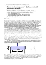
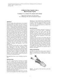
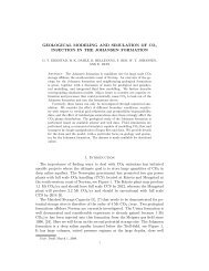
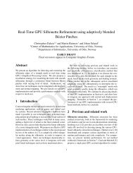
space and for each realization determining the partition it belongs to. Also,when basis functions that correspond to the same interface in the coarse gridare nearly linear dependent, then the number of basis functions may be reduced,e.g., by removing the basis functions that are at a very small angle (with respectto (·(λk) −1 , ·)) to the space spanned by the remaining basis functions associatedwith the same interface. These techniques reduce the computation cost withoutlosing essential information.5.2 Gaussian fieldsFor Gaussian fields, one can reduce the dimension of the uncertainty spacedramatically due to the fast decay of eigenvalues. To sample the realizations thatare used to generate the multiscale basis functions, we use the 1st order Smolyakcollocation points θ k in [−3, 3] L (see e.g., [32]). That is, θ 0 = 0, θ 2i−1 = 3δ ij ,and θ 2i = −3δ ij , i = 1, ..., L. We note that the choice of interpolation pointsdoes not affect the implementation of our approach.Our first results are for isotropic case with l 1 = l 2 = 0.2 and σ 2 = 2. In thiscase we can reduce the dimension of the stochastic permeability to 10. Fromthis stochastic model for the permeability we randomly draw 100 realizationsand perform simulations on the corresponding permeability fields.In Figure 1 we compare breakthrough times and cumulative oil productionat 0.6 PVI. We see that there is nearly a perfect match between the resultsobtained with mixed MsFEM and the corresponding results derived from thereference solutions. Next, in Figure 2, we plot L 2 errors in the saturation fieldfor these realizations as well as the water-cut errors. It can be observed fromthis figure that the saturation errors are mostly below 3%. Finally, we plot inFigure 3 a histogram of the breakthrough times and cumulative oil productionvalues depicted in Figure 1 to demonstrate that the mixed MsFEM essentiallyprovides the same statistics as one obtains from the set of reference solutions.These results suggest that with a few pre-computed basis functions in eachcoarse grid block we can solve two-phase flow equations on the coarse grid foran arbitrary realization and obtain nearly the same results, and hence nearly thesame statistics, as one obtains by doing fine grid simulations for each realization.In our next numerical example, we consider an anisotropic Gaussian fieldwith l 1 = 0.5, l 2 = 0.1 and σ 2 = 2. Due to anisotropy, it requires 12 terms inKLE. Again we sample the realizations that are used to generate the multiscalebasis functions using the 1st order Smolyak collocation points θ k in [−3, 3] L . Forillustration purposes, we plot in Figure 4 one randomly chosen realization andcorresponding saturation profiles at 0.6 PVI obtained by solving the pressureequation on the fine grid, and on the 5 × 5 coarse grid with the mixed MsFEM,respectively. We note that the depicted saturation profiles are approximatelythe same, even though the multiscale method solves the pressure equation on agrid that is coarsened 20 times in each direction.The numerical results obtained for the anisotropic Gaussian fields are qualitativelythe same as the results shown in Figure 1 – Figure 3. We thereforeinclude only the anisotropic equivalent of Figure 3. Histograms of breakthrough13

0.50.4Breakthrough times at producerMultiscale solutionReference solution0.30.20.100 10 20 30 40 50 60 70 80 90 1000.70.6Realization numberCumulative oil−production at 0.6 PVIMultiscale solutionReference solution0.50.40.30.20 10 20 30 40 50 60 70 80 90 100Realization numberFigure 1: Breakthrough time and cumulative oil production at 0.6 PVI for 100random realizations from a Gaussian field with l 1 = l 2 = 0.2 and σ 2 = 2.0.10.090.08Overall saturation error and water cut errorSaturation errorWater−cut error0.070.060.050.040.030.020.0100 10 20 30 40 50 60 70 80 90 100Figure 2: L 2 errors of the saturation field and water-cut errors for 100 randomlychosen realizations. Gaussian field with l 1 = l 2 = 0.2, σ 2 = 2.3530Histogram of breakthrough times at producerMultiscale solutionReference solutionHistogram of cumulative oil−production at 0.6 PVI30Multiscale solutionReference solution25252020151510105500 0.05 0.1 0.15 0.2 0.25 0.3 0.3500.2 0.25 0.3 0.35 0.4 0.45 0.5 0.55Figure 3: Histograms of the breakthrough times and cumulative oil productionvalues shown in Figure 1.14

time and cumulative oil production at 0.6 PVI for 100 randomly chosen realizationsare depicted in Figure 5. The histograms confirm that the multiscalemethod essentially provides the same breakthrough time and cumulative oilproduction statistics as one obtains from the set of reference solutions.5.3 Exponential variogram fieldsFor our second set of results, we consider permeability fields with exponentialcovariance matrix(R(x, y) = σ 2 exp − |x 1 − y 1 |− |x 2 − y 2 |). (5.5)l 1 l 2Because of slow decay of eigenvalues, one usually needs to keep many terms inthe KLE and deal with a large uncertainty space. For instance, for approximatingpermeability fields, KLE may require 300 to 400 eigenvectors depending oncorrelation lengths and variance. The KLE therefore gives a stochastic distributionin which it is very difficult to derive and employ interpolation formulas.Thus, for this problem our approach based on the mixed MsFEM offers a majoradvantage relative to interpolation based approaches. In fact, in our approachwe can simply select a few independent realizations and use these realizationsto build the approximation space V h , and then perform statistical studies ona much larger set of realizations. We note that for independent realizations,we do not have interpolation formula easily available. Moreover, the use of independentrealizations is quite easy and one can use this technique for moregeneral permeability fields since it only requires independent samples of thepermeability field.To demonstrate the performance of the stochastic multiscale method forthese fields, we present results for a case where the permeability fields are drawnfrom an anisotropic exponential variogram distribution with l 1 = 0.5, l 2 = 0.1,and σ 2 = 2 (the results for the isotropic case are similar, and not reported here).The KLE requires 350 eigenvectors to represent this stochastic permeability distribution.From this distribution we sample 20 independent realizations and usethese realizations to generate the multiscale basis functions. Figure 6 displaysone randomly chosen realization and corresponding saturation profiles at 0.6PVI obtained by solving the pressure equation on the fine grid, and on the 5 ×5coarse grid with the mixed MsFEM, respectively.Figures 7, 8, and 9, show; breakthrough time at producer and cumulativeoil production at 0.6 PVI for 100 randomly chosen realizations for both thereference solution and the multiscale solution; relative overall saturation errorand water-cut error; histograms of the breakthrough times and cumulative oilproduction values depicted in Figure 7. Figure 7 demonstrates that there isgenerally a good match between the breakthrough time and cumulative oil productioncurves for the reference and multiscale solutions. However, we nowobserve that there is a slight bias in the multiscale results, e.g., there is a smalltime-lag in the breakthrough times for the multiscale method. The bias canalso be observed from the histograms in Figure 9, but the magnitude of the bias15

Logarithm of permeability1.52040608010010 20 30 40 50 60 70 80 90 10010.50−0.5−1−1.5−2Reference saturation solution at 6.000000e−01 PVI2040608010010 20 30 40 50 60 70 80 90 100Multiscale saturation solution at 6.000000e−01 PVI2040608010010 20 30 40 50 60 70 80 90 100Figure 4: A Gaussian permeability field with l 1 = 0.5, l 2 = 0.1, σ 2 = 2, and acomparison of the reference saturation field and the saturation profile obtainedwith the multiscale method at 0.6 PVI.3025Histogram of breakthrough times at producerMultiscale solutionReference solutionHistogram of cumulative oil−production at 0.6 PVIMultiscale solutionReference solution2020151510105500 0.05 0.1 0.15 0.2 0.25 0.3 0.3500.2 0.25 0.3 0.35 0.4 0.45 0.5 0.55Figure 5: Histograms of breakthrough time and cumulative oil production at0.6 PVI for 100 random Gaussian fields with l 1 = 0.5 and l 2 = 0.1 and σ 2 = 2.16

1020304050Logarithm of permeability43210−11020304050Reference saturation solution1020304050Multiscale saturation solution60−2606070−3707080−4808090−5909010020 40 60 80 10010020 40 60 80 10010020 40 60 80 100Figure 6: An exponential variogram field with l 1 = 0.5, l 2 = 0.1, and σ 2 = 2, anda comparison of the reference saturation field at 0.6 PVI and the correspondingsaturation field obtained using the stochastic multiscale method.is small, and the multiscale solutions are generally quite close to the referencesolution, as is illustrated in Figure 6 and Figure 8.We now demonstrate that the bias in breakthrough time and cumulativeoil production persists, but is efficiently reduced by increasing the number ofrealizations used to generate the multiscale basis functions. Figures 10, 11,and 12 show, respectively, the saturation and water-cut error for each of the100 realization for the stochastic multiscale method with different sample sizes,the cumulative probability distribution of breakthrough times and cumulativeoil production, and the corresponding histograms of the breakthrough timesand the cumulative oil production values. The plots show the following; thesaturation and water-cut errors decay with increasing sample size; the timelag in the breakthrough times (also observed in the cumulative oil production)decays rapidly with increasing sample size, and that using 50 basis functionsfor each coarse grid interface generates statistics that are nearly unbiased, andgenerally match the statistics derived from the set of reference solutions verywell. Observe that a sample size of 50 gives rise to a linear system with 2025unknowns, roughly 1/15 as many as in the fine grid system.5.4 Uncertainty quantificationWe would like to note that the proposed techniques can be effectively used inuncertainty quantification based on methods proposed in [20]. Our goal in [20]is to sample the permeability from the distributionπ(k) ∝ exp(− 1 ∫ Ts 2 (q w (t) − q obs (t)) 2 dt),0where q w is the water-cut corresponding to the permeability field k, q obs isobserved water-cut, T is the time of available history and s is the error precision.In [20], multi-stage Markov chain Monte Carlo methods are proposed, wherethe first stage involves inexpensive simulations. These simulations are used to17

0.40.350.30.250.20.150.1Breakthrough times at producerMultiscale solutionReference solution0.050 10 20 30 40 50 60 70 80 90 100Realization numberCumulative oil−production at 0.6 PVI0.5Multiscale solutionReference solution0.40.30.20 10 20 30 40 50 60 70 80 90 100Realization numberFigure 7: Breakthrough time and cumulative oil production at 0.6 PVI for 100random realizations from an exponential variogram field with l 1 = 0.5, l 2 = 0.1,and σ 2 = 2.0.30.25Overall saturation error and water cut errorSaturation errorWater−cut error0.20.150.10.0500 10 20 30 40 50 60 70 80 90 100Figure 8: L 2 errors of the saturation field and water-cut errors for 100 randomlychosen exponential variogram fields with l 1 = 0.5, l 2 = 0.1, and σ 2 = 2.353025Histogram of breakthrough times at producerMultiscale solutionReference solutionHistogram of cumulative oil−production at 0.6 PVI45Multiscale solution40Reference solution3530202515201051510500 0.05 0.1 0.15 0.2 0.25 0.3 0.3500.2 0.25 0.3 0.35 0.4 0.45 0.5Figure 9: Histograms of the breakthrough times and cumulative oil productionvalues shown in Figure 7.18

Overall saturation error0.50.40.3Sample size = 10Sample size = 20Sample size = 30Sample size = 500.20.100 10 20 30 40 50 60 70 80 90 100Water−cut error0.250.20.15Sample size = 10Sample size = 20Sample size = 30Sample size = 500.10.0500 10 20 30 40 50 60 70 80 90 100Figure 10: Saturation and water-cut error for solutions obtained using differentnumber of permeability realizations to generate the multiscale basis functions.100908070Cumulative distribution function for breakthrough times at producerSample size = 10Sample size = 20Sample size = 30Sample size = 50Reference solution100908070Cumulative distribution function for cumulative production at 0.6 PVISample size = 10Sample size = 20Sample size = 30Sample size = 50Reference solution60605050404030302020101000.05 0.1 0.15 0.2 0.25 0.3 0.35PVI00.25 0.3 0.35 0.4 0.45 0.5PVIFigure 11: Cumulative probability distribution for breakthrough time and cumulativeoil production at 0.6 PVI.403530Histogram of breakthrough times at producerSample size = 10Sample size = 20Sample size = 30Sample size = 50Reference solution403530Histogram of cumulative oil−production at 0.6 PVISample size = 10Sample size = 20Sample size = 30Sample size = 50Reference solution25252020151510105500 0.05 0.1 0.15 0.2 0.25 0.3 0.3500.2 0.25 0.3 0.35 0.4 0.45 0.5 0.55Figure 12: Histograms of the breakthrough times and cumulative oil production.19

2.5Cross plot21.5π(k)10.500 0.5 1 1.5 2 2.5π * (k)Figure 13: Cross plot between π(k) and π ∗ (k).screen the fine-scale runs. Our main goal is to provide such inexpensive coarsescaleruns that are statistically accurate. Our initial numerical results showthat the proposed methods can be efficiently used in these application. One ofthe main criteria for these inexpensive simulations is strong correlation betweenπ(k) and π ∗ (k), where π ∗ (k) is approximate distribution. In Figure 13, we plotthe cross plot of ∫ T0 (q w(t) −q obs (t)) 2 dt for fine-scale and multiscale simulations.The strong correlation suggests that our approach can be successfully used inthese uncertainty quantification problems. One can also test less expensivemethods where the saturation equation is solved on the coarse grid or faststreamline techniques are used. These inexpensive computations are observedto be statistically accurate in [20, 16] when realization based multiscale finiteelement type methods are used. In future, we will study the stochastic mixedMsFEM combined with the upscaled transport equations.6 ConclusionsIn this paper, our goal is to develop mixed multiscale finite element methods(MsFEM) for solving stochastic flow equations described by second order ellipticequations with random coefficients. The proposed approaches computemultiscale basis functions on the coarse spatial grid. The pre-computed basisfunctions are constructed based on selected realizations of the stochastic permeabilityfield, and thus span both spatial scales and uncertainties. These basisfunctions are used to solve the stochastic equation for an arbitrary realizationon the coarse grid.20

We consider mixed formulation of the flow problem. The solution is projectedonto the finite dimensional space spanned by pre-computed basis functions.The proposed method can be regarded as an extension of mixed MsFEM tostochastic porous media flow equations. We employ multiscale methods usinglimited global information since the permeability fields do not have apparentscale separation. The proposed approach does not require any interpolation instochastic space and can accurately predict the solution on the coarse grid. Ingeneral, the uncertainty space can be partitioned into coarse regions where ourapproach can be used in each coarse patch.We present numerical results for two-phase immiscible flow in stochasticporous media. In particular, we consider both Gaussian fields as well as permeabilityfields with exponential variogram. For the former case, due to smalleruncertainty space, we use lowest order interpolation points in uncertainty spacefor computing the basis functions. For the exponential case, due to large uncertainties,we employ randomly selected realizations for constructing basis functions.Numerical results show that for both cases, one can accurately predictthe solutions with the multiscale method using only a few realizations to generatebasis functions. It is particularly encouraging that the proposed multiscalemethods are capable of predicting the stochastic solution with very few basisfunctions in high dimensional uncertainty space. We would like to note thatthe proposed approaches are not restricted to Cartesian grids and can be usedfor unstructured grids [4]. Finally, we would like to note that the proposed approachescan be easily combined with interpolation based approaches in orderto achieve greater flexibility.Although the results presented in this paper are encouraging, there is scopefor further exploration. Our intent here was to demonstrate that one can capturethe spatial and uncertainty variations of the stochastic flow solutions via precomputedbasis functions. In particular, we would like to show that the methodprovides a foundation for fast simulations for a large number of realizationsneeded for the calculation of flow and transport statistics. Our initial numericalresults show that the proposed approaches can be efficiently used to speed-upthe uncertainty quantification problems of subsurface flows. Our future aim isto use the stochastic mixed MsFEM in preconditioning of Markov chain MonteCarlo simulations. In particular, we will study the statistical accuracy of theapproaches where mixed MsFEM combined with both coarse-scale and fine-scalesaturation solvers.7 AcknowledgmentThe research of J. A. is funded by the Research Council of Norway under grantno. 158908/I30 and by Shell and the Research Council of Norway under grant no.175962/S30. The research of Y. E. is partially supported by NSF CMG/DMSgrant 0621113 and DOE grant DE-FG02-05ER25669. We are grateful to PaulDostert for performing initial numerical simulations on uncertainty quantificationusing the proposed mixed multiscale finite element method.21

References[1] J. E. Aarnes, On the use of a mixed multiscale finite element methodfor greater flexibility and increased speed or improved accuracy in reservoirsimulation, SIAM MMS, 2 (2004), pp. 421–439.[2] J. E. Aarnes, Y. Efendiev, and L. Jiang, Analysis of multiscale finiteelement methods using global information for two-phase flow simulations,(submitted to Comp. Geo.)[3] J. E. Aarnes, Y. Efendiev, and L. Jiang,Analysis of Multiscale FiniteElement Methods using Global Information For Two-Phase Flow Simulations,submitted to SIAM MMS.[4] J. E. Aarnes, S. Krogstad, and K.-A. Lie, A hierarchical multiscalemethod for two-phase flow based upon mixed finite elements and nonuniformgrids, Multiscale Model. Simul. 5(2) (2006), pp. 337–363.[5] J. E. Aarnes, S. Krogstad, and K.-A. Lie, Multiscale mixed/mimeticmethods on corner-point grids, To appear in Comput. Geosci.[6] T. Arbogast, Implementation of a locally conservative numerical subgridupscaling scheme for two-phase Darcy flow, Comput. Geosci., 6 (2002),pp. 453–481. Locally conservative numerical methods for flow in porousmedia.[7] T. Arbogast, G. Pencheva, M. F. Wheeler, and I. Yotov, A multiscalemortar mixed finite element method, SIAM J. Multiscale Modelingand Simulation, to appear.[8] I. Babu˘ska, G. Caloz, and E. Osborn, Special finite element methodsfor a class of second order elliptic problems with rough coefficients, SIAMJ. Numer. Anal., 31 (1994), pp. 945–981.[9] I. Babu˘ska and E. Osborn, Generalized finite element methods: Theirperformance and their relation to mixed methods, SIAM J. Numer. Anal.,20 (1983), pp. 510–536.[10] F. Brezzi, Interacting with the subgrid world, in Numerical analysis 1999(Dundee), Chapman & Hall/CRC, Boca Raton, FL, 2000, pp. 69–82.[11] Y. Chen and L. Durlofsky, An ensemble level upscaling approach for efficientestimation of fine-scale production statistics using coarse-scale simulations,SPE paper 106086, presented at the SPE Reservoir SimulationSymposium, Houston, Feb. 26-28 (2007).[12] Y. Chen, L. J. Durlofsky, M. Gerritsen, and X. H. Wen, A coupledlocal-global upscaling approach for simulating flow in highly heterogeneousformations, Advances in Water Resources, 26 (2003), pp. 1041–1060.22

[13] Z. Chen and T. Y. Hou, A mixed multiscale finite element methodfor elliptic problems with oscillating coefficients, Math. Comp., 72 (2002),pp. 541–576 (electronic).[14] C. V. Deutsch and A. G. Journel, GSLIB: Geostatistical softwarelibrary and user’s guide, 2nd edition, Oxford University Press, New York,1998.[15] P. Dostert Uncertainty quantification using multiscale methods for porousmedia flows, Ph.D. thesis, Texas A& M University, 2007.[16] P. Dostert, Y. Efendiev, T. Hou, and W. Luo,, Coarse-gradientLangevin algorithms for dynamic data integration and uncertainty quantification,J. Comp. Physics, 217 (2006), pp. 123-142.[17] W. E and B. Engquist, The heterogeneous multi-scale methods, Comm.Math. Sci., 1(1) (2003), pp. 87–133.[18] Y. Efendiev, V. Ginting, T. Hou, and R. Ewing, Accurate multiscalefinite element methods for two-phase flow simulations, J. Comp. Physics,220 (1), pp. 155-174, 2006.[19] Y. Efendiev, T. Hou, and V. Ginting, Multiscale finite element methodsfor nonlinear problems and their applications, Comm. Math. Sci., 2(2004), pp. 553–589.[20] Y. Efendiev, T. Hou and W. Luo, Preconditioning Markov chain MonteCarlo simulations using coarse-scale models, SIAM. Sci. Comp. 28(2), pp.776-803, 2006.[21] Y. Efendiev, T. Y. Hou, and X. H. Wu, Convergence of a nonconformingmultiscale finite element method, SIAM J. Num. Anal., 37 (2000),pp. 888–910.[22] T. Y. Hou and X. H. Wu, A multiscale finite element method for ellipticproblems in composite materials and porous media, Journal of ComputationalPhysics, 134 (1997), pp. 169–189.[23] T. Hughes, G. Feijoo, L. Mazzei, and J. Quincy, The variationalmultiscale method - a paradigm for computational mechanics, Comput.Methods Appl. Mech. Engrg, 166 (1998), pp. 3–24.[24] P. Jenny, S. H. Lee, and H. Tchelepi, Multi-scale finite volume methodfor elliptic problems in subsurface flow simulation, J. Comput. Phys., 187(2003), pp. 47–67.[25] M. Loève, Probability Theory, 4th ed., Springer, Berlin, 1977.23

[26] F. Nobile, R. Tempone, and C. G. Webster, A sparse grid stochasticcollocation method for elliptic partial differential equations with randominput data, MOX Technical Report 85, Dipartimento di Matematica, submittedto SIAM Journal of Numerical Analysis (2006).[27] D. Oliver, L. Cunha, and A. Reynolds, Markov chain Monte Carlomethods for conditioning a permeability field to pressure data, MathematicalGeology, 29 (1997).[28] H. Owhadi and L. Zhang, Metric based up-scaling, Comm. Pure Appl.Math., 2007.[29] P. Raviart and J. Thomas, A mixed finite element method for secondorder elliptic equations, In: I. Galligani and E. Magenes (eds.): MathematicalAspects of Finite Element Methods. Berlin – Heidelberg – New York:Springer–Verlag, pp. 292–315, 1977.[30] C. Robert and G. Casella, Monte Carlo Statistical Methods, Springer-Verlag, New-York, 1999.[31] E. Wong, Stochastic Processes in Information and Dynamical Systems,MCGraw-Hill, 1971.[32] D. Xiu and J. Hesthaven, High-Order Collocation Methods for DifferentialEquations with Random Inputs, SIAM J. Sci. Comput. Wol. 27, No.3, pp. 1118-1139.24