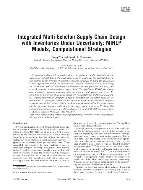
Integrated multi-echelon supply chain design with inventories under ...

Integrated Multi-Echelon Supply Chain Designwith Inventories Under Uncertainty: MINLPModels, Computational StrategiesFengqi You and Ignacio E. GrossmannDept. of Chemical Engineering, Carnegie Mellon University, Pittsburgh, PA 15213DOI 10.1002/aic.12010Published online September 15, 2009 in Wiley InterScience (www.interscience.wiley.com).We address in this article a problem that is of significance to the chemical industry,namely, the optimal design of a multi-echelon supply chain and the associated inventorysystems in the presence of uncertain customer demands. By using the guaranteedservice approach to model the multi-echelon stochastic inventory system, we developan optimization model to simultaneously determine the transportation, inventory, andnetwork structure of a multi-echelon supply chain. The model is an MINLP with a nonconvexobjective function including bilinear, trilinear, and square root terms. Byexploiting the properties of the basic model, we reformulate this problem as a separableconcave minimization program. A spatial decomposition algorithm based on theintegration of Lagrangean relaxation and piecewise linear approximation is proposedto obtain near global optimal solutions with reasonable computational expense. Examplesfor specialty chemicals and industrial gas supply chains with up to 15 plants, 100potential distribution centers, and 200 markets are presented. VC 2009 American Instituteof Chemical Engineers AIChE J, 56: 419–440, 2010Keywords: supply chains, mixed-integer programming, inventory control, Lagrangeandecomposition, industrial gasesIntroductionA recent report released by US Census Bureau shows thatthe total value of inventory in United States is around $1.4trillion (10% of US GDP), 1 of which around 24% are contributedby the chemical process industry. Another report bySmartOps shows that more than 50% of these inventories areinefficient. 2 Thus, there is a great economic incentive tooptimize the inventories across process supply chains. 3,4 Toaccomplish this objective, the main challenge is how toeffectively integrate inventory management with networkdesign for multi-echelon process supply chains, so that decisionson locations to stock the inventory and the associatedamount of inventories can be determined simultaneously tominimize costs. The integration is nontrivial for multi-echelonsupply chains and their associated inventory systems inCorrespondence concerning this article should be addressed to I. E. Grossmann atgrossmann@cmu.eduVC2009 American Institute of Chemical Engineersthe presence of uncertain customer demands. 5 This problemhas not been addressed before.Although inventory management is a very important problemfor the process industry, most of the models in thechemical engineering literature consider inventory managementand supply chain network design separately. On theother hand, there are related works on supply chain optimizationthat take into account the inventory costs, but considerinventory issues coarsely without detailed inventorymanagement policy. 6–10 In these models, the safety stocklevel is given as a parameter and usually treated as a lowerbound of the total inventory level 11–19 or it is considered asan inventory target that would lead to some penalty costs ifviolated. 20 This approach cannot optimize the safety stocklevels, especially when considering demand uncertainty.Thus, it can only provide an approximation of the inventorycost and may lead to suboptimal solutions.Research on integrated supply chain network design andstochastic inventory management is relatively new. Most ofthe existing literature focuses on ‘‘single stage’’ inventoryAIChE Journal February 2010 Vol. 56, No. 2419

structure integrated with supply chain design, but withoutextending it to ‘‘multi-echelon’’ inventory systems addressedin this work. Daskin et al. 21 and Shen et al. 22 present a jointlocation-inventory model, which extends the classical uncapacitatedfacility location model to include nonlinear workinginventory and safety stock costs for a two-stage supplychain network, so that decisions on the installation of distributioncenters (DCs) and the detailed inventory replenishmentdecisions are jointly optimized. To simplify the problem,inventories in the retailers are neglected and they alsoassume that all the DCs have the same constant replenishmentlead time, and the demand at each customer has thesame variance-to-mean ratio. With the same assumptions,Ozsen et al. 23 have extended the model to consider capacitatedlimits in the DCs. Their work is further extended byOzsen et al. (submitted for publication) to compare with thecases in which customers restrict to single sourcing and thecase in which customers allow multi-sourcing. Anotherextension is given by Sourirajan et al. 24 in which theassumption of identical replenishment lead time is relaxed,whereas the assumption on demand uncertainty is stillenforced. Recently, You and Grossmann 6 proposed a mixedintegernonlinear programming (MINLP) approach to study amore general model based on the one developed by Daskinet al. 21 and Shen et al. 22 relaxing the assumption on identicalvariance-to-mean ratio for customer demands.The objective of this work is to develop optimizationmodels and solution algorithms to address the problem ofjoint multi-echelon supply chain network design and inventorymanagement. By using the guaranteed service approachto model the time delays in the material flows in the multiecheloninventory system, 7–10,25–30 we capture the stochasticnature of the product deliveries at each stage (echelon) ofthe supply chain and develop an equivalent deterministicoptimization model. The model determines the supply chaindesign decisions (including the locations of DCs, assignmentsof customer demand zones to DCs, assignments ofDCs to plants), shipment levels from plants to the DCs andfrom DCs to customers, and inventory decisions such aspipeline inventory and safety stock in each node of the supplychain network. The model also captures risk-poolingeffects 31 by consolidating the safety stock inventory ofdownstream nodes to the upstream nodes in the multi-echelonsupply chain. The model is first formulated as a mixedintegernonlinear program (MINLP) with a nonconvex objectivefunction and then reformulated as a separable concaveminimization program after exploiting the properties of thebasic model. To solve the problem efficiently, a tailored spatialdecomposition algorithm based on Lagrangean relaxationand piece-wise linear approximation is developed to obtainnear global optimal solutions within 1% optimality gap withmodest CPU times. Several computational examples forindustrial gases supply chains and specialty chemical supplychains are presented to illustrate the application of the modeland the performance of the proposed algorithm.This article includes several novel features. First, we explicitlymodel the multi-echelon inventory system of a processsupply chain under demand uncertainty and use a holisticapproach to simultaneously optimize the supply chaindesign decisions and multi-echelon stochastic inventory managementdecisions. To the best of our knowledge, the integrationof multi-echelon stochastic inventory with supplychain design has not been addressed before, as most of theliterature on joint supply chain design and inventory managementconsiders only single-echelon inventory system.Capturing the multi-echelon inventory structure allows us toconsider variable replenishment lead times and inventoryallocation issues, both of which can significantly improvethe decision-making across the process supply chains. Second,we develop a novel and efficient global optimizationalgorithm to obtain solutions within 1% global optimalitygap for the resulting large scale nonconvex MINLP instanceswith thousands of discrete and continuous variables, andmore than one million constraints. The proposed algorithm isbased on effective integration of piece-wise linear approximationand Lagrangean relaxation that as far as we knowhas not been considered before. The entire solution processrequires only a mixed-integer linear programming (MILP)solver without the need of an NLP solver. The efficientglobal optimization algorithm that allows large-scale solutionand does not rely on nonlinear solvers is therefore anothercontribution of this work.The outline of this article is as follows. Some basic conceptsof inventory management with risk pooling and theguaranteed service model for multi-echelon inventory systemare presented in Section Multi-Echelon Inventory. The problemstatement is given in Section 3. In Section Model Formulation,we introduce the joint multi-echelon supply chaindesign and inventory management model. Two small illustrativeexamples are given in Section 5. To solve the largescale problem, an efficient decomposition algorithm basedon Lagrangean relaxation and piecewise linear approximationis presented in Section Solution Algorithm. Our computationalresults and analysis are given in Section 7. We concludethis article in the last section.Multi-Echelon Inventory ModelIn this section, we briefly review some inventory managementmodels that are related to the problem addressed inthis work. Detailed discussion about single-stage and multiecheloninventory management models are given by Zipkin 5and Graves and Willem, 27 respectively.Single-stage inventory model under base-stock policyThere are many control policies for single-stage inventorysystems, such as base stock policy, (s,S) policy, (r, Q) policy,etc. 5 Among these policies, the periodic review base stock policyis the most widely used in the practice of inventory control.The reason is based on two facts. As shown by Federgruenand Zipkin, 32 the base stock policy is optimal for singlestageinventory system facing stationary demand. For multiecheloninventory systems, the base stock policy, although notnecessarily optimal, has the advantage of being simple toimplement and close to the optimum. 33 Before introducing themulti-echelon inventory model, we first review the single-stagebase stock policy, which is the common building block formost of the multi-echelon inventory models.Figure 1 shows the inventory profile for a given productin a stocking facility operated under the periodic reviewbase stock policy. As can be seen, the inventory level420 DOI 10.1002/aic Published on behalf of the AIChE February 2010 Vol. 56, No. 2 AIChE Journal

this field is to assume a normal distribution of the demand,although of course other distribution functions can be specified.If the demand at each unit of time is normally distributedwith mean l and standard deviation r, due to the propertyof normal distribution, the demand over review period pand the replenishment lead time l is also normally distributedwith meanpl(p þ l) and variance r 2 (p þ l) (standard deviationrffiffiffiffiffiffiffiffiffiffi p þ l). It is convenient to measure safety stock interms of the number of standard deviations of demanddenoted as safety stock factor, k. Thenpthe optimal basestock level is given by S ¼ lðp þ lÞþkrffiffiffiffiffiffiffiffiffiffi p þ l, as shownin Figure 2.We should note that if a is the Type I service level (theprobability that the total inventory on hand is more than thedemand) used to measure of service level, the safety stockfactor k corresponds to the a-quantile of the standard normaldistribution, i.e., Pr(x k) ¼ a.Figure 1. Inventory profile under base stock policy.(a) Deterministic demand case. (b) Under demand uncertainty.[Color figure can be viewed in the online issue,which is available at www.interscience.wiley.com.]decreases due to the customer demand and increases whenreplenishments arrive. Under the periodic review base stockpolicy, inventory is reviewed at the beginning of eachreview period and the difference between a specified basestock level and the actual inventory position (on-hand inventoryplus in-process inventory minus backorders) is orderedfor replenishment. It is interesting to note that the wellknowncontinuous review (r, Q) policy can be treated as aspecial case of base stock policy with base stock level equalto r þ Q, where r is the reorder point of inventory level andQ is the order quantity.As under the base stock policy, the lengths of the reviewperiod and the replenishment lead time are determined exogenously,the only control variable is the base stock level. Todetermine the optimal base stock level for a single-stage inventorysystem, let us denote the review period as p, thereplenishment lead time as l, and the average demand ateach unit of time as l. Recall that the inventory position isthe total material in the system (on-hand plus on-order), andwe start each review period with the same inventory positionS, which is the base stock level. We must wait p units oftime to review the inventory position again and place anorder for replenishment, and then the order will take anotherl units of time to arrive (Figure 1). Therefore, the inventoryin the system at the beginning of a review period should belarge enough to cover the demand over review period p plusthe replenishment lead time l, i.e., the optimal base stocklevel should be l(p þ l) if demand is deterministic as in Figure1a.Under demand uncertainty, we need more inventory(safety stock) to hedge against stockout before we get achance to reorder as in Figure 1b. The accepted practice inRisk pooling effectFor single-echelon inventory system with multiple stockinglocations, Eppen 31 proposed the ‘‘risk pooling effect,’’which states that significant safety stock cost can be savedby grouping in one central location the demand of multiplestocking locations. In particular, Eppen considers a singleperiod problem with N retailers and one supplier. Eachretailer i has uncorrelated normally distributed demand withmean l i and standard deviation r i . The review periods andreplenishment lead times for all these retailers are the sameand given as p and l, respectively. All the retailers guaranteethe same Type I service level with the same safety stock factork. Eppen compared two operational modes of the N-retailer system: decentralized mode and centralized mode. Inthe decentralized mode, each retailer orders independently tominimize its cost. As in this mode, the optimal safety stockinpretailer i corresponding to the safety stock factor k iskffiffiffiffiffiffiffiffiffiffipp þ lr i , 31 the total safety stock in the system is given bykffiffiffiffiffiffiffiffiffiffi Pp þ l Ni¼1 r i. In the centralized mode, all the retailers areconsidered as a whole and a single quantity is ordered forreplenishment, so as to minimize the total expected cost ofthe entire system. As in the centralized mode, all theFigure 2. Safety stock level for normally distributeddemand over lead time.[Color figure can be viewed in the online issue, which isavailable at www.interscience.wiley.com.]AIChE Journal February 2010 Vol. 56, No. 2 Published on behalf of the AIChE DOI 10.1002/aic 421

Figure 3. Timing relationship in guaranteed serviceapproach.[Color figure can be viewed in the online issue, which isavailable at www.interscience.wiley.com.]retailers are grouped and the demand at each retailer followsa normal distribution N(l i , r 2 i ), the total uncertain demandof the entire system during the order lead time will also followa normal distribution with mean (p þ l) P Ni¼1l i andpffiffiffiffiffiffiffiffiffiffiqffiffiffiffiffiffiffiffiffiffiffiffiffiffiffiffiPstandard deviation p þ l Ni¼1 r2 i . Therefore, the totalsafety stock of the distribution centers in the centralizedpmode is given by kffiffiffiffiffiffiffiffiffiffi qffiffiffiffiffiffiffiffiffiffiffiffiffiffiffiffiPp þ l Ni¼1 r2 i , which is less thanpkffiffiffiffiffiffiffiffiffiffi Pp þ l Ni¼1 r i. Eppen’s simple model illustrates the potentialsaving in safety stock costs because of risk pooling. Forexample, consider a single-echelon inventory system with100 retailers. Each retailer has uncorrelated normal distributeddemand with identical mean l and standard deviationpr. Thus, the total safety stock of this system is 100zr ffiffiffiffiffiffiffiffiffiffi p þ lpunder decentralized mode, and only 10zrffiffiffiffiffiffiffiffiffiffi p þ l under centralizedmode, i.e., 90% safety stocks in this system can besaved by risk pooling.Guaranteed service model for multi-echelon inventoryOne of the most significant differences between singlestageinventory system and multi-echelon inventory systemis the lead time. For single-stage inventory system, leadtime, which may include material handling time and transportationtime, is exogenous and generally can be treated asa parameter. However, for a multi-echelon inventory system,lead time of a downstream node depends on the upstreamnode’s inventory level and demand uncertainty, and thus thelead time and internal service level are stochastic. Based onthis fact, simply propagating the single-stage inventorymodel to multi-echelon system leads to suboptimal solutionsbecause the optimization of a multi-echelon inventory systemis usually nontrivial. 5There are two major approaches to model the multi-echeloninventory system, the stochastic service approach and theguaranteed service approach. 27 For a detailed comparison ofthese two approaches, see Graves and Willems 27 and Humairand Willems. 29 In this work, we choose the guaranteed serviceapproach to model the multi-echelon inventory system.Definitions in guaranteed service approachThe main idea of the guaranteed service approach is thateach node j in the multi-echelon inventory system quotes aguaranteed service time T j , by which this node will satisfythe demands of material flow from its downstream customers.That is, the customer demand at time t must be ready tobe shipped by time t þ T j . The guaranteed service times forinternal customers are decision variables to be optimized,whereas the guaranteed service time for the nodes at the lastechelon (facing external customers) is an exogenous input,which can be treated as a parameter. Besides the guaranteedservice time, we consider that each node has a given deterministicorder processing time, t j , which is independent ofthe order size. The order processing time, t j , which includesmaterial handling time, transportation time, and review period,represents the time from all the inputs that are readyuntil the outputs are available to serve the demand. Therefore,the replenishment lead time, which represents the timefrom when we place an order to when all the goods arereceived, can be determined by the guaranteed service timeof the direct predecessor T j 1 (the time that predecessorrequires to have the chemicals ready to be shipped) plus theorder processing time t j . As we can see from Figure 3, thenet lead time of node j, NLT j , which is the required timespan to cover demand variation using safety stocks at node j,is defined as the difference between the replenishment leadtime of this node and its guaranteed service time to its successor.10 The reason is that not all the customer demand attime t for node j should be satisfied immediately, but onlyneeds to be ready by time t þ T j . Thus, the safety stockdoes not need to cover demand variations over the entirereplenishment lead time, but just the difference between thereplenishment lead time and the guaranteed service time tothe successors, i.e., the net lead time. Therefore, we can calculatenet lead time with the following formula:NLT j ¼ T j 1 þ t j T jwhere node j 1 is the direct predecessor of node j. Note thatthis formula implies that if the service time quoted by node j toits successor nodes equals the replenishment lead time, T j 1 þt j , i.e., NLT j ¼ 0 as shown in Figure 4a, no safety stock isrequired in node j because all products are received from thepredecessors and processed within the guaranteed service time,i.e., this node is operating in ‘‘pull’’ mode. If the guaranteedservice time T j is 0, i.e., NLT j ¼ T j 1 þ t j as shown in Figure4b, the node holds the most safety stock because all the orders,once they are placed, are fulfilled immediately, i.e., this nodeis operating in ‘‘push’’ mode.Figure 4. Extreme net lead times.(a) Zero, no safety stock. (b) Largest, highest safety stock.[Color figure can be viewed in the online issue, which isavailable at www.interscience.wiley.com.]422 DOI 10.1002/aic Published on behalf of the AIChE February 2010 Vol. 56, No. 2 AIChE Journal

PI j ¼ t j l jwhich is not affected by the coverage and guaranteed servicetime decisions.Figure 5. Motivating example of a series inventory systemwith a plant, a DC, and a market withfixed times to illustrate the timing relationships.[Color figure can be viewed in the online issue, which isavailable at www.interscience.wiley.com.]Optimal based stock level and inventory cost ofguaranteed service approachIn the guaranteed service approach, each node in themulti-echelon inventory system is assumed to operate undera periodic review base stock policy with a common reviewperiod. Furthermore, demand over any time interval is alsoassumed to be normally distributed (mean l j and standarddeviation r j for node j) and ‘‘bounded.’’ This does notimply that demand can never exceed the bound, but thisbound reflects the maximum amount of demand that acompany wants to satisfy from safety stock. This interpretationis consistent with most practical applications thatsafety stocks are used to cope with regular demand variationsthat do not exceed a maximum reasonable bound.Larger demand variations are handled with extraordinarymeasures, such as spot-market purchases, rescheduling orexpediting orders, other than using safety stocks. Thus,under these assumptions, each node sets its base stock soas to meet all the orders from its downstream customerswithin the guaranteed service time. That is, for node j thereis an associated safety stock factor k j , which is given andcorresponds to the maximum amount of demand that companywants to satisfy from safety stock. This yields thebase stock level at node j:pffiffiffiffiffiffiffiffiffiffiffiS j ¼ l j NLT j þ k j r j NLT jThis formula is similar but slightly different from the single-stageinventory model in terms of the expression for the lead time. Notethat the review period has been taken into account as part of theorder processing time and considered in the net lead time.With the guaranteed service approach, the total inventorycost consists of safety stock cost and pipeline inventory cost.The safety stock of node j (SS j ) is given by the followingformula as discussed earlier,pffiffiffiffiffiffiffiffiffiffiffiSS j ¼ k j r j NLT jThe expected pipeline inventory is the sum of expected onhand and on-order inventories. Based on Little’s law, 34 theexpected pipeline inventory PI j of node j equals to the meandemand over the order processing time and is given by,Example of a series inventory systemTo illustrate the main idea of guaranteed service approach,let us consider an example of a series inventory system withone plant, one DC, and one market as in Figure 5. In thisexample, the plant has a guaranteed service time of 2 days,which quantitatively represents the worst case supply uncertaintyand production delay. It means that every order from theDC will be satisfied in at most 2 days, regardless of the uncertaintyand delay from supply and production. The guaranteedservice time of the market is zero, which means that everyproduct in the market should be ready to be used immediately.Thus, the guaranteed service time of the plant is usually determinedexogenously based on supply uncertainty and productiondelay, whereas the guaranteed service time of market isalso exogenously determined by the market requirement.In this way, the major decision variable of this system isthe guaranteed service time of the DC. As shown in Figure6a, the summation of plant’s guaranteed service time andorder processing time from plant to DC leads to the DC’sworst case replenishment lead time, 5 days, which is thetime span from the DC receives an order until the order isready to be shipped out from the DC. Therefore, if the DCcommits a guaranteed service time the same as the worstcase replenishment lead time, 5 days, there is no need tohold safety stock in the DC because every order from themarket requires at most 5 days to be fulfilled. In this case,the DC is operated under the ‘‘pull’’ mode and the net leadtime is zero. Another extreme case is that the DC commits azero guaranteed service time. In this case, the optimal safetystock should be able to cover the demand uncertainty overthe worst case replenishment lead time because every orderfrom the market should be satisfied immediately.As the guaranteed service time increases from 0 to 5 days(the worst case replenishment lead time), the net lead time,which is the difference between worst case replenishment leadtime and guaranteed service time, decreases from 5 days to 0,and consequently the optimal safety stock level decreases fromthe maximum level to zero, as in Figures 6b, c. Therefore, theguaranteed service time of the DC is an important decision variablethat can adjust the optimal safety stock level in the DC.Besides, the DC’s guaranteed service time also affects thesafety stock level of the market. As shown in Figure 7, themarket’s net lead time equals to the DC’s guaranteed servicetime plus the order processing time from DC to customer.For instance, if the DC’s guaranteed service time is 4 days,the market should hold sufficient safety stock to hedge thedemand uncertainty over 6 days, which is the worst casereplenishment lead time of the market. Thus, the majorobjective is to find out the optimal guaranteed service time,so as to reduce the total cost based on the adjusting the inventoryallocation decisions between the DC and the market.Problem StatementWe are given a potential supply chain (Figure 8) for agiven chemical product that consists of a set of plants (orAIChE Journal February 2010 Vol. 56, No. 2 Published on behalf of the AIChE DOI 10.1002/aic 423

Figure 7. The timing relationship between plant, DCand market in the motivating example.[Color figure can be viewed in the online issue, which isavailable at www.interscience.wiley.com.]Figure 6. The relationship between times and safetystock level of the DC in the motivatingexample.(a) Replenishment lead time, guaranteed service time andnet lead time of the DC in the motivating example. (b) Conceptualrelationship between safety stock level and guaranteedservice time of DC. (c) Conceptual relationshipbetween safety stock level and net lead time of DC. [Colorfigure can be viewed in the online issue, which is availableat www.interscience.wiley.com.]suppliers) i [ I, a number of candidate sites for distributioncenters j [ J, and a set of customer demand zones k [ K,whose inventory costs should be taken into account. Thecustomer demand zone can represent a distributor, a warehouse,a dealer, a retailer, or a wholesaler, which is usuallya necessary component of the supply chain for specialtychemicals or advanced materials. 25,35 Alternatively, onemight view the customer demand as the aggregation of agroup of customers operated with vendor managed inventory(vendor takes care of customers’ inventory), which is a commonbusiness model in the industrial gases industry andsome chemical companies. 36,37In the given potential supply chain, the location of theplants, potential distribution centers, and customer demandzones are known and the distances between them are given.The investment costs for installing DCs are expressed by acost function with fixed charges. Each retailer i has anuncorrelated normally distributed demand with mean l i andvariance r 2 iin each unit of time. Single sourcing restriction,which is common in industrial gases supply chains 36,37 andspecialty chemicals supply chains, 38 is employed for the distributionfrom plants to DCs and from DCs to customerdemand zones. That is, each DC is only served by one plant,and each customer demand zone is only assigned to one DCto satisfy the demand. Linear transportation costs areincurred for shipments from plant i to distribution center jwith unit cost c1 ij and from distribution center j to customerdemand zone k with unit cost c2 jk . The corresponding deterministicorder processing times of DCs and customerdemand zone, which includes the material handling time,transportation time, and inventory review period, are givenby t1 ij and t2 jk . The service time of each plant and theFigure 8. Supply chain network structure (three echelons).[Color figure can be viewed in the online issue, which isavailable at www.interscience.wiley.com.]424 DOI 10.1002/aic Published on behalf of the AIChE February 2010 Vol. 56, No. 2 AIChE Journal

maximum service time of each customer demand zonesare known. We are also given the safety stock factorfor DCs and customer demand zones, k1 j and k2 k , whichcorrespond to the standard normal deviate of the maximumamount of demand that the node will satisfy from itssafety stock. A common review period is used for the controlof inventory in each node. Inventory costs areincurred at distribution centers and customers, and consist ofpipeline inventory and safety stock, of which the unit costsare given.The problem is then to determine how many distributioncenters (DCs) to install, where to locate them, which plantsto serve each DC, and which DCs to serve each customerdemand zone, how long should each DC quote its servicetime, and what level of safety stock to maintain at each DCand customer demand zone so as to minimize the total installation,transportation, and inventory costs.We should note that the guaranteed service time is only avariable for the DCs, and hence the net lead times are variablesfor the DCs and customer demand zones. Therefore, theproblem corresponds effectively to a three-echelon supplychain with inventories under uncertainty.Model FormulationThe joint multi-echelon supply chain design and inventorymanagement model for a given chemical product can be formulatedas a mixed-integer nonlinear program (MINLP).The definition of sets, parameters, and variables of the modelare given latter.Sets/IndicesI ¼ set of plants (suppliers) indexed by iJ ¼ set of candidate DC locations indexed by jK ¼ set of customer demand zones (wholesaler, regionaldistributor, dealer, retailer, or customers with vendor managedinventory) indexed by kParametersc1 ij ¼ unit transportation cost from plant i to DC jc2 jk ¼ unit transportation cost from DC j to customerdemand zone kf j ¼ fixed cost for installing a DC at candidate location j(annually)g j ¼ variable cost coefficient for installing candidate DC j(annually)h1 j ¼ unit inventory holding cost at DC j (annually)h2 k ¼ unit inventory holding cost at customer demandzone k (annually)R k ¼ maximum guaranteed service time to customers atcustomer demand zone kSI i ¼ guaranteed service time of plant it1 ij ¼ order processing time of DC j if it is served byplant i, including material handling time of DC j, transportationtime from plant i to DC j, and inventory review periodt2 jk ¼ order processing time of customer demand zone kif it is served by DC j, including material handling time ofDC j, transportation time from DC j to customer demandzone k, and inventory review periodl k ¼ mean demand at customer demand zone k (daily)r 2 k ¼ variance of demand at customer demand zone k(daily)v ¼ days per year (to convert daily demand and variancevalues to annual costs)h1 ij ¼ unit cost of pipeline inventory from plant i to DC j(annual)h2 jk ¼ unit cost of pipeline inventory from DC j to customerdemand zone k (annual)k1 j ¼ safety stock factor of DC jk2 k ¼ safety stock factor of customer demand zone kBinary variables (0–1)X ij ¼ 1ifDCj is served by plant i and 0 otherwiseY j ¼ 1 if we install a DC in candidate site j and 0 otherwiseZ jk ¼ 1 if customer demand zone k is served by DC j and0 otherwiseContinuous variables (0 to 1‘)L k ¼ net lead time of customer demand zone kN j ¼ net lead time of DC jS j ¼ guaranteed service time of DC j to its successive customerdemand zonesAuxiliary variables (0 to 1‘)XZ ijk ¼ the product of X ij and Z jkSZ jk ¼ the product of S j and Z jkSZ1 jk ¼ auxiliary variable for linearizationNZ jk ¼ the product of N j and Z jkNZ1 jk ¼ auxiliary variable for linearizationNZV j ¼ auxiliary variable for reformulationu1 j,p1 ¼ auxiliary variable for piecewise linear approximationu2 k,p2 ¼ auxiliary variable for piecewise linear approximationu3 j,k,p3 ¼ auxiliary variable for piecewise linear approximationW j ¼ objective function value of problem (APL j )bW j ¼ objective function value of problem (APLR j )W j ¼ objective function value of problem (APLP j )Auxiliary variables (0–1)v1 j,p1 ¼ auxiliary variable for piecewise linear approximationv2 k,p2 ¼ auxiliary variable for piecewise linear approximationv3 j,k,p3 ¼ auxiliary variable for piecewise linear approximationObjective FunctionThe objective of this model is to minimize the total supplychain design cost including the following items:• Installation costs of DCs.• Transportation costs from plants to DCs and from DCsto customer demand zones.• Pipeline inventory costs in DCs and customer demandzones.• Safety stock costs in DCs and customer demand zones.AIChE Journal February 2010 Vol. 56, No. 2 Published on behalf of the AIChE DOI 10.1002/aic 425

The cost of installing a DC in candidate location j isexpressed by a fixed-charge cost model that captures theeconomies of scale in the investment. The annual expecteddemand of DC j is ( P k[K vZ jk l k ), which equals to the annualmean demand of all the customer demand zones k [ Kserved by DC j. Hence, the cost of installing DC j consistsof fixed cost f j and variable cost (g jPk[K vZ jk l k ), which isthe product of variable cost coefficient and the expecteddemand of this DC in 1 year. Thus, the total installationcosts of all the DCs is given by,Xf j Y j þ X 89X>: g j vZ jk l k >; (1)j2J j2JThe product of the annual mean demand of DC j ( P k[K vZ jk l k ) and the unit transportation cost ( P i[Ic1 ij X ij ) betweenplant i and DC j yields the annual plant to DC transportationcost.89X X X>: c1 ij X ij vZ jk l k >; (2)i2Ij2JSimilarly, the product of yearly expected mean demand ofcustomer demand zone k (vl k ) and the unit transportation cost( P j[Jc2 jk Z jk ) between customer demand zone k leads to theannual DC to customer demand zone transportation cost.X Xc2 jk vZ jk l k (3)j2Jk2KBased on Little’s law, 34 the pipeline inventory PI j of DC jequals to the product of its daily mean demand ( P k[KZ jk l k )and its order processing time ( P i[It1 ij X ij ) which is given interms of days. Thus, the annual total pipeline inventory cost ofall the DCs is given by,89X X X>: h1 j t1 ij X ij Z jk l k >; (4)i2Ij2Jwhere h1 j is the annual unit pipeline inventory holding cost ofDC j.Similarly, the total annual pipeline inventory cost of allthe customer demand zones is given by,k2Kk2Kk2KX Xh2 k t2 jk Z jk l k (5)j2Jk2Kwhere h2 k is the annual unit pipeline inventory holding cost ofcustomer demand zone k and P k[Kt2 jk Z jk l k is the pipelineinventory of customer demand zone k.The demand at customer demand zone k follows a givennormal distribution with mean l k and variance r 2 k . Becauseof the risk-pooling effect, 31 the demand over the net leadtimeP(N j )atDCj is also normally distributed with a mean ofN j k[J kl k and a variance of N jPk[J kr 2 k , in which J k is theset of customer demand zones k assigned to DC j. Thus, thesafety stock required in the DC at candidate location j withpffiffiffiffiffiqffiffiffiffiffiffiffiffiffiffiffiffiffiffiffiffiffiffiffiffiffiffiPa safety stock factor k1 j is k1 j N j k2K r2 k Z jk. Consideringthe annual inventory holding cost at DC j is h1 j , wehave the total annual safety stock cost at all the DCsequals toX pffiffiffiffiffirffiffiffiffiffiffiffiffiffiffiffiffiffiffiffiffiffiffiXk1 j h1 j N j r 2 k Z jk(6)j2JSimilarly, the demand over the net lead time L k of customerdemand zones k is normally distributed with a mean of L k l kand a variance of L k r 2 k. Thus, the annual safety stock cost at allthe customer demand zones is given by,X pffiffiffiffiffik2 k h2 k r k L k(7)k2KTherefore, the objective function of this model (total supplychain design cost) is given byXmin : f j Y j þ X 89X>: g j vZ jk l k >;j2J j2J k2Kþ X 89X X>: c1 ij X ij vZ jk l k >; þ X Xc2 jk vZ jk l ki2I j2Jk2Kj2J k2Kþ X 89X X>: h1 j t1 ij X ij Z jk l k >; þ X Xh2 k t2 jk Z jk l ki2I j2Jk2Kj2J k2Kþ X pffiffiffiffiffirffiffiffiffiffiffiffiffiffiffiffiffiffiffiffiffiffiffiXk1 j h1 j N j r 2 k Z jk þ X pffiffiffiffiffik2 k h2 k r k L kj2Jk2Kk2Kwhere each term accounts for the DC installation cost,transportation costs of plants-DCs and DCs-customer demandzones, pipeline inventory costs of DCs and customer demandzones, and safety stock costs of DCs and customer demand zones.ConstraintsThree types of constraints are used to define the networkstructure. The first one is that if DC j is installed, it shouldbe served by only one plant i. If the DC is not installed, it isnot assigned to any plant. This can be modeled by,XX ij ¼ Y j ; 8j (9)i2IThe second constraint states that each customer demand zone kis served by only one DC,XZ jk ¼ 1; 8k (10)j2JThe third constraint is that if a customer demand zone k isserved by the DC in candidate location j, the DC must exist,k2K(8)Z jk Y j ; 8j; k (11)Two constraints are used to define the net lead time of the DCsand customer demand zones. The replenishment lead time ofDC j should be equal to the guaranteed service time (SI i )ofplant i, which serves DC j, plus the order processing time (t ij ).Note that the guaranteed service time (SI i ) of plant i is treated426 DOI 10.1002/aic Published on behalf of the AIChE February 2010 Vol. 56, No. 2 AIChE Journal

as parameters and represents the worst case supply uncertaintyand production delay of plants. As each DC is served by onlyonePplant, the replenishment lead time of DC j is calculated byi[I(SI i þ t ij ) X ij . Thus, the net lead time of DC j should begreater than its replenishment lead time minus its guaranteedservice time to its successor customer demand zones, S j , whichis a variable.N j X ðSI i þ t1 ij ÞX ij S j ; 8j (12)i2ISimilarly, the net lead time L k of a customer demand zone k isgreater than its replenishment lead time minus its maximumguaranteed service time, R k , which is given by the nonlinearinequalityL k X ðS j þ t2 jk ÞZ jk R k ; 8k (13)j2JNote that in this article we consider R k as parameters, althoughthis formulation can be extended to a bi-criterion optimizationmodel by treating R k as variables to simultaneously minimizethe total cost and responsiveness.Finally, all the decision variables for network structure arebinary variables, and the variables for guaranteed servicetime and net lead time are non-negative variables.MINLP ModelX ij ; Y j ; Z jk 2f0; 1g; 8i; j; k (14)S j 0; N j 0; 8j (15)L k 0; 8k (16)Grouping the parameters, we can rearrange the objectivefunction and formulate the problem as the following mixedintegernonlinear program (P0):Min :s:t:Xf j Y j þ X X XA ijk X ij Z jk þ X XB jk Z jkj2J i2I j2J k2K j2J k2Kþ X rffiffiffiffiffiffiffiffiffiffiffiffiffiffiffiffiffiffiffiffiffiffiffiXq1 j N j r 2 k Z jk þ X p ffiffiffiffiffi (17)q2 k L kj2Jk2Kk2KN j X i2IS ij X ij S j ; 8j (12)q1 j ¼ k1 j h1 jq2 k ¼ k2 k h2 k r kReformulated MINLP ModelThe MINLP model (P0) has nonconvex terms, includingbilinear and square root terms, in its objective function (17)and constraint (13). Because the bilinear terms are the productsof two binary variables (such as X ij Z jk ) or the productsof a binary variable and a continuous variable (such asN j Z jk and S j Z jk ), they can be linearized by introducingadditional variables.To linearize the term (X ij Z jk ) in the objective function(17), we first introduce a new continuous non-negative variableXZ ijk . Then the product of X ij and Z jk can be replacedby this term XZ ijk with the following constraints, 39XZ ijk X ij ; 8i; j; k (19)XZ ijk Z jk ; 8i; j; k (20)XZ ijk X ij þ Z jk 1; 8i; j; k (21)XZ ijk 0; 8i; j; k (22)where constraints (19), (20), and (22) ensure that if X ij or Z jk iszero, XZ ijk should be zero, whereas constraint (21) ensures thatif X ij and Z jk are both equal to one, XZ ijk should be one.The linearization of (S j Z jk ) in constraint (13) requirestwo new continuous non-negative variable SZ jk and SZ1 jk ,and the following constraints, 39SZ jk þ SZ1 jk ¼ S j ; 8j; k (23)SZ jk Z jk S U j ; 8j; k (24)SZ1 jk ð1 Z jk ÞS U j ; 8j; k (25)SZ jk 0; SZ1 jk 0; 8j; k (26:1)where constraints (24), (25), and (26.1) ensure that if Z jk iszero, SZ jk should be zero; if Z jk is one, SZ1 jk should be zero.Combining with constraint (23), we can have SZ jk equivalentto the product of S j and Z jk .Similarly, the product of N j and Z jk in the objective function(17) can be linearized as follows,NZ jk þ NZ1 jk ¼ N j ; 8j; k (27)whereL k X ðS j þ t2 jk ÞZ jk R k ; 8k (13)j2JConstraints ð9Þ ð11Þ; ð14Þ ð16ÞS ij ¼ SI i þ t1 ijA ijk ¼ c1 ij v þ h1 j t1 ij lkB jk ¼ g j v þ c2 jk v þ h2 k t2 jk lkNZ jk Z jk Nj U ; 8j; k (28)NZ1 jk ð1 Z jk ÞNj U ; 8j; k (29)NZ jk 0; NZ1 jk 0; 8j; k (26:2)where NZ jk and NZ1 jk are two new continuous variables, andNZ jk is equivalent to (N j Z jk ).The above linearizations introduce more constraints andvariables, significantly reduce the number of nonlinear termsin the model (P0) and potentially reduce the computationaleffort. To further reduce the nonlinear terms in the objectivefunction (17), the term (N j P k[K r 2 k Z jk) is replaced by aAIChE Journal February 2010 Vol. 56, No. 2 Published on behalf of the AIChE DOI 10.1002/aic 427

secants in the objective function (17) will lead to the MILPproblem (P2) with a linear objective function,Min :Xf j Y j þ X X XA ijk XZ ijk þ X XB jk Z jkj2J i2I j2J k2K j2J k2Kþ X q1 j NZV jqffiffiffiffiffiffiffiffiffiffiffiffiþ X q2 k L kqffiffiffiffiffiffij2J NZVjU k2K L U k(34)Figure 9. Secant of a univariate square root term.[Color figure can be viewed in the online issue, which isavailable at www.interscience.wiley.com.]new nonnegative continuous variable NZV j with the followingconstraint,NZV j ¼ X k2Kr 2 k NZ jk; 8j (30)NZV j 0; 8j (31)Therefore, incorporating the above linearizations, we have thefollowing reformulated MINLP model (P1).Min :Xf j Y j þ X X XA ijk XZ ijk þ X XB jk Z jkj2J i2I j2J k2K j2J k2Kþ X pffiffiffiffiffiffiffiffiffiffiq1 j NZV j þ X p ffiffiffiffiffi (17)q2 k L kj2Jk2Ks:t: L k X SZ jk þ X t2 jk Z jk R k ; 8k (32)j2J j2JConstraints ð9Þ ð11Þ; ð14Þ ð16Þ; and ð18Þ ð31ÞCompared with model (P0), model (P1) is computationallymore tractable because all the constraints in (P1) are linearand the only nonlinear terms are univariate concave terms inthe objective function.Initialization ProcessThe bounds of variables are quite important for nonlinearoptimization problems. Tight upper bounds of the key continuousvariables are given in the Appendix section. Besidesvariable bounds, a good initial solution is another key issuefor numerical optimization of MINLP problems, as it providesa tight upper bound of the objective and consequentlyreduces the search space and computational time. As model(P1) has some special structure (linear constraints, univariateconcave terms in the objective function), we can use a similarapproach as in You and Grossmann 6 to obtain a ‘‘good’’initial solution by solving a (MILP) approximation for initializationpurposes.As introduced bypFalk and Soland 40 for a univariatesquare root termffiffi x , in which the variable p x has lowerbound 0 and upper bound x U , its secant x=ffiffiffiffiffix U representsthe convex envelope and provides a valid lower bound ofthe square root term as shown in Figure 9. As model (P1) isa minimization problem and all the constraints are linear,replacing all the univariate square root terms with theirs.t. all the constraints of (P1)As (P1) and (P2) have the same constraints, a feasible solutionof (P2) is also a feasible solution of (P1). Furthermore,the optimal objective function value of (P2) is a validlower bound of the optimal objective function value of (P1).Therefore, by solving the initialization MILP problem (P2),we can obtain a ‘‘good’’ initial solution for problem (P1)and a tight upper bound of the objective.Note that based on this initialization procedure, a heuristicalgorithm is to first solve problem (P2), then using its optimalsolution as an initial point to solve problem (P1) withan MINLP solver that relies on convexity assumption (e.g.,DICOPT, SBB). This algorithm can obtain ‘‘good’’ solutionsquickly, although global optimality cannot be guaranteed(actually it provides a valid upper bound of the global optimalsolution).Illustrative ExamplesTo illustrate the application of the MINLP model (P1), weconsider two small illustrative examples, an industrial liquidoxygen (LOX) supply chain example and an acetic acid supplychain example.Example A: Industrial LOX supply chainThe first example is for an industrial LOX supply chainwith two plants, three potential DCs, and six customers asgiven in Figure 10. In this supply chain, customer inventoriesare managed by the vendor, i.e., vendor-management-Figure 10. LOX supply chain network superstructurefor Example A.[Color figure can be viewed in the online issue, which isavailable at www.interscience.wiley.com.]428 DOI 10.1002/aic Published on behalf of the AIChE February 2010 Vol. 56, No. 2 AIChE Journal

Table 1. Parameters for Demand Uncertaintyfor Example AMean Demand l i(liters/day)Standard Deviationr i (liters/day)Customer 1 257 150Customer 2 86 25Customer 3 194 120Customer 4 75 45Customer 5 292 64Customer 6 95 30inventory (VMI), which is a common business model in thegas industry. 35–37 Thus, in this example inventory costs fromDCs and customers should be taken into account in the totalsupply chain cost, and the joint multi-echelon supply chaindesign and inventory management model can be used tominimize total network design, transportation, and inventorycosts.In this instance, the annual fixed costs to install the threeDCs (f j ) are $10,000 per year, $8,000 per year, and $12,000per year, respectively. The variable cost coefficient of installinga DC (g j ) at all the candidate locations is $0.01 per liter/year.The safety stock factors for DCs (k1 j ) and customers(k2 k ) are the same and equal to 1.96, which correspondsto 97.5% service level if the demand is normally distributed.We consider 365 days in a year (v). The guaranteed servicetimes of the two plants (SI i ) are 2 days and 3 days, respectively.As the last echelon represents the customers, theguaranteed service time of customers (R k ) are set to 0. Thedata for demand uncertainty, order processing times, andtransportation costs are given in Tables 1–5.We consider two instances of this example. In the firstinstance, we consider zero holding cost for both pipeline inventoryand safety stocks, i.e., the problem reduces to a supplychain network design problem without considering inventorycost. In the second instance, the pipeline inventoryholding cost of LOX is $6 per liter/year for all the DCs(h1 ij ) and customers (h2 jk ), and the safety stock holding costis $8 per liter/year for all the DCs (h1 j ) and customers (h2 k ).Both the initialization MILP model (P2) and the MINLPmodel (P1) involve 27 binary variables, 124 continuous variables,and 256 constraints. As the problem sizes are relativelysmall, we solve model (P1) directly to obtain theglobal optimum with 0% optimality margin by using theBARON solver 41 with GAMS, 42 and the initialization MILPmodel (P2) is solved with GAMS/CPLEX. The resultingoptimal supply chain networks with a minimum annual costof $108,329/year and the flow rate of each transportationlink are given in Figure 11a. We can see that for theinstance without considering inventory costs, all the threeDCs are installed, and each of them serves two customers.The major trade-off is between DC installation costs and thetransportation costs. For the instance taking into account theTable 3. Order Processing Time (t2 jk ) Between DCs andCustomers (Days)Cust. 1 Cust. 2 Cust. 3 Cust. 4 Cust. 5 Cust. 6DC1 2 2 3 3 4 4DC2 4 4 1 1 4 4DC3 4 4 3 3 2 2inventory costs, only two DCs are installed, and each servesthree customers as seen in Figure 11b. The major trade-offis between DC installation costs, transportation costs, and inventorycosts. The minimum annual cost in this instance is$152,107/year with the variable cost items given in Figure12. A comparison between these two instances suggests theimportance of integrating inventory costs in the supply chainnetwork design.The optimal net lead times and guaranteed service timesof DCs and customers for the design in Figure 11b are givenin Figure 13. We can see in Figure 13a that in the path ofmaterial flow from Plant 2 to DC 1 and to Customers 1, 2,and 3, DC 1 has an optimal service time equal to the plant’sservice time plus the deterministic order processing timefrom Plant 2 to DC 1, i.e., 5 days. Note that this servicetime corresponds to the worst case response time from plantto DC, although the most optimistic case is that Plant 2 willfulfill the demand immediately and the minimum responsetime will be the deterministic order processing time, i.e., 2days. We can observe similar phenomena in the path of materialflow from Plant 1 to DC 3 and to Customers 4, 5, and6 from Figure 13b. As both DC 1 and DC 3 have the optimalservice times equal to the summation of plant’s servicetime and the order processing time between plants and DCs,both of them have zero net lead time, i.e., do not hold anysafety stock and work as pure ‘‘pull’’ systems. In Figures14a, b, we can see that all the customers in the optimal solutionhave positive net lead times and hold sufficient safetystocks to ensure their guaranteed service times are zero, i.e.,work as pure ‘‘push’’ system. This interesting phenomenashows that safety stock allocation of the multi-echelon LOXsupply chain leads to a hybrid ‘‘push – pull’’ systems, inwhich each node either does not hold inventory or holdsmaximum required inventory, and the ‘‘pull’’ and ‘‘push’’boundary is between the DCs and the customers. What weobserved in this example is consistent and similar to the onediscovered by Simpson 30 for multistage ‘‘series’’ inventorysystem. It is also interesting to note that all the optimal guaranteedservice times and net lead times happen to be integer,although we do not restrict them to be integer values.Example B: Acetic acid supply chainThe second example is for an acetic acid supply chainwith three plants, three potential DCs, and four customerTable 2. Order Processing Time (t1 ij ) Between Plants andDCs (Days) for Example ADC1 DC2 DC3Plant 1 7 4 2Plant 2 2 4 7Table 4. Unit Transportation Cost (Cl ij ) fromPlants to DCs ($/liter)DC1 DC2 DC3Plant 1 0.24 0.20 0.20Plant 2 0.18 0.19 0.23AIChE Journal February 2010 Vol. 56, No. 2 Published on behalf of the AIChE DOI 10.1002/aic 429

Table 5. Unit Transportation Cost (c2 jk ) from DCs toCustomers ($/liter)Cust. 1 Cust. 2 Cust. 3 Cust. 4 Cust. 5 Cust. 6DC1 0.01 0.03 0.10 0.44 1.60 2.30DC2 1.50 0.25 0.01 0.02 0.25 1.50DC3 2.27 1.73 0.51 0.10 0.01 0.03demand zones, each of which has a wholesaler (Figure 15).On the basis of the conclusion of the previous example, weneed to take into account the inventory costs from DCs andwholesalers when designing the optimal supply chain.In this instance, the annual fixed DC installation cost (f j )is $50,000 per year for all the DCs. The variable cost coefficientof installing a DC (g j ) at all the candidate locations is$0.5 per ton/year. The safety stock factors for DCs (k1 j ) andwholesalers (k2 k ) are the same and equal to 1.96. We consider365 days in a year (v). The guaranteed service times ofthe three plants (SI i ) are 3, 3, and 4 days, respectively. Thepipeline inventory holding cost is $1 per ton/day for all theDCs (h1 ij /v) and wholesalers (h2 jk /v), and the safety stockFigure 12. Cost items of the LOX supply chain inExample A.[Color figure can be viewed in the online issue, which isavailable at www.interscience.wiley.com.]holding cost is $1.5 per ton/day for all the DCs (h1 j /v) andwholesalers (h2 k /v). The guaranteed service time of wholesalersto end customers (R k ) is set to be 8 days. The data forFigure 11. Optimal network structure for the LOX supplychain in Example A.(a) Without considering inventory costs, total cost ¼$108,329. (b) Considering inventory costs, total cost ¼$152,107. [Color figure can be viewed in the online issue,which is available at www.interscience.wiley.com.]Figure 13. Optimal timing relationship of the LOX supplychain for the design in Figure 8b.(a) Plant 2: DC 1 – Customers 1, 2, and 3. (b) Plant 1:DC 3 – Customers 4, 5, and 6. [Color figure can beviewed in the online issue, which is available at www.interscience.wiley.com.]430 DOI 10.1002/aic Published on behalf of the AIChE February 2010 Vol. 56, No. 2 AIChE Journal

Table 6. Parameters for Demand Uncertainty for Example BMean Demandl i (ton/day)Standard Deviationr i (ton/day)Wholesaler 1 250 150Wholesaler 2 180 75Wholesaler 3 150 80Wholesaler 4 160 45Figure 14. Optimal net lead times and safety stock levelsof the LOX supply chain for the design inFigure 8b.(a) Net lead times and guaranteed service times of DCsand customers. (b) Optimal safety stock levels of DCs andcustomers. [Color figure can be viewed in the online issue,which is available at www.interscience.wiley.com.]demand uncertainty, order processing times, and transportationcosts are given in Tables 6–10.The computational study is carried out on an IBM T40laptop with Intel 1.50GHz CPU and 512 MB RAM. Theoriginal model (P0) has 12 discrete variables, 22 continuousvariables, and 27 constraints. Both the initialization MILPmodel (P2) and the MINLP model (P1) involve 24 binaryvariables, 185 continuous variables, and 210 constraints. Wesolve the original model (P0) by using GAMS/BARON with0% optimality margin, and it takes a total of 1376.9 CPUseconds. We then solve the reformulated model (P1) withthe aforementioned initialization process, the CPU timereduces to only 7.6 s and the optimal solutions are the sameas we obtained by solving model (P0). The possible reasonis that initialization process helps BARON to find a ‘‘good’’feasible solution during the preprocessing step. This solutionprovides a tighter upper bound that reduces the search spaceand speeds up the computation.The resulting optimal supply chain network with a minimumannual cost of $1,986,148 per year and the flow ratesof transportation links are given in Figure 16. We can seethat two DCs are selected to install and one of them servesthree wholesalers whereas the other one only serves onewholesaler. The major trade-off is between DC installationcosts, transportation costs, and inventory costs. A detailedbreakdown of the total cost is given in Figure 17.Figure 18 shows the optimal net lead times and guaranteedservice times of DCs and wholesalers. Because themaximum guaranteed service time of the wholesalers is setto be 8 days, whereas the total deterministic time from plant2 to DC 1 and to Wholesaler 1 is only 7 days, it is reasonablethat this path work as pure ‘‘pull’’ system to reduce thetotal inventory cost as in Figure 18a. In Figure 18b, we cansee that for the path from Plant 1 to DC 2 and to Wholesalers2, 3, and 4, Wholesaler 4 requires a significantly longorder processing time (4 days) compared with others (1 dayonly). Therefore, it is understandable that most of the safetystocks are maintained in Wholesaler 1, although other nodesin this path also work as pure ‘‘pull’’ system. As seen inFigure 19, similarly as in the previous example, it can beobserved that most of the nodes in this supply chain holdzero safety stock and work as pure ‘‘pull’’ system. The inventoryallocation in this example also suggests the importanceof incorporating multi-echelon stochastic inventorysystem in the supply chain design. Instead of focusing onthe single-stage inventory only, the proposed approach canlead to an explicit improvement of the decision-making insupply chain design, and in turn reduce the total costs.Solution AlgorithmAlthough small-scale problems can be solved to globaloptimality effectively by using a global optimizer, mediumTable 7. Order Processing Time (t1 ij ) Between Plants andDCs (Days) for Example BFigure 15. Acetic acid supply chain network superstructurefor Example B.[Color figure can be viewed in the online issue, which isavailable at www.interscience.wiley.com.]DC1 DC2 DC3Plant 1 4 4 2Plant 2 2 4 3Plant 3 3 4 4AIChE Journal February 2010 Vol. 56, No. 2 Published on behalf of the AIChE DOI 10.1002/aic 431

Table 8. Order Processing Time (t2 jk ) Between DCs andWholesalers (Days)Wholesaler 1 Wholesaler 2 Wholesaler 3 Wholesaler 4DC1 2 2 3 3DC2 4 4 1 1DC3 4 4 3 3Table 10. Unit Transportation Cost (c2 jk ) from DCs toWholesalers ($/Ton)Wholesaler 1 Wholesaler 2 Wholesaler 3 Wholesaler 4DC1 1.0 3.3 4.0 7.4DC2 1.0 0.5 0.1 2.0DC3 7.7 7.3 5.1 0.1and large-scale joint multi-echelon supply chain design andinventory management problems are often computationallyintractable with direct solution approaches because of thecombinatorial nature and nonlinear nonconvex terms. In thissection, we present an effective solution algorithm based onthe integration of Lagrangean relaxation and piecewise linearapproximation to obtain solutions within 1% of global optimalitygap with reasonable computational expense.Piecewise Linear ApproximationInstead of using the secants in the objective function ofmodel (P1), a tighter lower convex envelope of the univariatesquare root terms is the piecewise linear function thatuses a few additional continuous and discrete variables.Although this may require longer computational times tosolve the initialization MILP problem, with the significantprogress of MILP solvers piecewise linear approximationshave recently been increasingly used for approximating differenttypes of nonconvex nonlinear functions, 43,44 especiallyfor univariate concave functions. 45–48There are several different approaches to model piecewiselinear function for a concave term. 44,47,49 In this work, weuse the ‘‘multiple-choice’’pformulation 47 to approximate thesquare root termffiffi x . Let P ¼ {1,2,3,…,p} denote the set ofintervals in the piecewise linear function u(x), and M 1 ,M 2 ,…, M p , M pþ1 be the lower and upper bounds of x foreach intervalpp. The ‘‘multiple choice’’ formulation ofuðxÞ ¼ffiffi x is given by,uðxÞ ¼mins:t:XðF p v p þ C p u p ÞpXv p ¼ 1pXu p ¼ xpM p v p u p M pþ1 v p ; p 2 Pv p 2 f0; 1g; p 2 PpffiffiffiffiffiffiffiffiffiffipffiffiffiffiffiffiM pþ1 M pwhere C p ¼andM pþ1 M ppF p ¼ffiffiffiffiffiffiM pC p M p ; p 2 P:As can be seen in Figure 20, the more intervals that are used,the better is the approximation of the nonlinear function, butmore additional variables and constraints are required. Usingthis ‘‘multiple-choice’’ formulation pffiffiffiffiffiffiffiffiffiffitopapproximateffiffiffiffiffithe univariateconcave terms NZV j and L k in the objectivefunction of problem (P1) yields the following piecewise linearMILP problem (P3), which provides a tighter lower boundingproblem for (P1).(P3):XMin : f j Y j þ X X XA ijk XZ ijk þ X XB jk Z jkj2J i2I j2J k2K j2J k2Kþ X Xq1 j F1 j;p1 v1 j;p1 þ C1 j;p1 u1 j;p1j2J p 1þ X X (35)q2 k F2 k;p2 v2 k;p2 þ C2 k;p2 u2 k;p2k2K p 2Xs:t: v1 j;p1 ¼ 1; 8j (36:1)p 1Xu1p 1¼ (36:2)j;p1 NZV j ; 8jM1 j;p1 v1 j;p1 u1 j;p1 M1 j;p1þ1v1 j;p1 ; 8j; p 1 (36:3)v1 j;p1 2 f0; 1g; u1 j;p1 0; 8j; p 1 (36:4)Xv2p 2¼ 1; 8k (37:1)k;p2Xp 2u2 k;p2 ¼ L k ; 8k (37:2)M2 k;p2 v2 k;p2 u2 k;p2 M2 k;p2 þ1v2 k;p2 ; 8k; p 2 (37:3)v2 k;p2 2 f0; 1g; u2 k;p2 0; 8k; p 2 (37:4)All the constraints of (P1).Table 9. Unit Transportation Cost (c1 ij ) from Vendors toDCs ($/Ton)DC1 DC2 DC3Vendor 1 1.8 1.6 2.0Vendor 2 2.4 2.2 1.3Vendor 3 2.0 1.3 2.5Figure 16. Optimal network structure for the aceticacid supply chain (Example B).[Color figure can be viewed in the online issue, which isavailable at www.interscience.wiley.com.]432 DOI 10.1002/aic Published on behalf of the AIChE February 2010 Vol. 56, No. 2 AIChE Journal

L jk S1 jk þ t jk Z jk R k Z jk ; 8j; k (41:1)L jk Z jk L U jk ; 8j; k (41:2)S j ¼ S1 jk þ S2 jk ; 8j; k (41:3)S1 jk Z jk S U j; 8j; k (41:4)S2 jk ð1 Z jk ÞS U j ; 8j; k (41:5)S1 jk 0; S2 jk 0; 8j; k (41:6)Figure 17. Cost items of the acetic acid supply chain inExample B.[Color figure can be viewed in the online issue, which isavailable at www.interscience.wiley.com.]Note that any feasible solution obtained from problem(P3) is also a feasible solution of (P1), and for each feasiblesolution the objective value of (P3) is always less than orequal to the objective value of (P1).In summary, the solution obtained by solving (P3) canprovide a ‘‘good’’ initial solution and tight upper bound ofsolving problem (P1). In addition, the optimal objectivevalue of (P3) provides a valid global lower bound to theobjective value of (P1).To obtain an initial point ‘‘close’’ enough to the global solution,we can in principle use piecewise linear functionswith sufficient large number of intervals to approximate theunivariate concave terms in (P1). However, it is a nontrivialtask to solve large-scale instances of (P3). To furtherimprove the computational efficiency, we first exploit someproperties of problem (P1).where S1 jk and S2 jk are two new auxiliary variables.The value of the new continuous variable L jk in (AP) isdefined through two new constraints (39) and (40). It meansthat if customer demand zone k is assigned to DC j, i.e., Z jk¼ 1, then the new variable L jk represents the net lead timeof customer demand zone k, otherwise L jk ¼ 0. Thus, anyfeasible solution of problem (AP) is also a feasible solutionof problem (P1), and vice versa, as stated in the followingproperty:Property 1. If (X * ij, Y * j,Z * jk, S * j,N * j,L * k) is a feasible solutionof problem (P1) with objective function value W * , then(X * ij, Y * j,Z * jk, S * j,N * j,L * jk), where L * jk ¼ 0ifZ * jk ¼ 0 and L * jk ¼L * k if Z * jk ¼ 1, is a feasible solution of problem (AP) and theassociated objective function value of (AP) is W * .If(X * ij, Y * j,Z * jk, S * j,N * j,L * jk) is a feasible solution of problem (AP) withobjective function value W * , then (X * ij, Y * j, Z * jk, S * j, N * j, L * k),where L * k ¼ P j [ JL * jk, is a feasible solution of problem (P1)and the associated objective function value of (P1) is W * .The property can be easily proved and is omitted in thisarticle. This property shows that we can solve either (P1) or(AP) to obtain a feasible or optimal solution, and then algebraicallyderive the solution to another problem with theAlternative FormulationLet us first consider an alternative model formulation (AP)of problem (P1) in which (23)–(25) are excluded and representthe inequality (13) by the disjunction (39),Min :Xf j Y j þ X X XA ijk XZ ijk þ X XB jk Z jkj2J i2I j2J k2K j2J k2Kþ X pffiffiffiffiffiffiffiffiffiffiq1 j NZV j þ X X p ffiffiffiffiffiffi (38)q2 k L jkj2Jj2Jk2Ks.t. Z jk:Z_ jk; 8j; k (39)L jk S j þ t jk R k L jk 0L jk 0; 8j; k (40)Constraints (9)-(11), (14)-(15), (18)-(22), and (27)-(31)Note that each disjunction in (39) is written in terms ofthe disaggregated variable L jk , which is then substituted inthe last term of the objective function (38). Applying theconvex hull reformulation 50,51 to the above disjunctive constraint(39) in (AP) leads to:Figure 18. Optimal timing relationship for the aceticacid supply chain in Example B.(a) Plant 2: DC 1 – Wholesaler 1. (b) Plant 1: DC 2 –Wholesalers 2, 3, and 4. [Color figure can be viewed inthe online issue, which is available at www.interscience.wiley.com.]AIChE Journal February 2010 Vol. 56, No. 2 Published on behalf of the AIChE DOI 10.1002/aic 433

where W is the objective function value. Note that problem(APL) can be decomposed into |J| subproblems, one foreach candidate DC site j [ J, where each one is denoted by(APL j ) and is shown for a specific subproblem for candidateDC site j as follows:W j ¼ Min : f j Y j þ X XA ijk XZ ijki2I k2Kþ X pffiffiffiffiffiffiffiffiffiffiB jk k k Zjk þ q1 j NZV j þ X p ffiffiffiffiffiffi (43)q2 k L jkk2Kk2KFigure 19. Net lead times and guaranteed service timesof DCs and wholesalers for the acetic acidsupply chain in Example B.[Color figure can be viewed in the online issue, which isavailable at www.interscience.wiley.com.]same objective value. Compared with model (P1), model(AP) has more square root terms in the objective functiondue to the introduction of variable L jk , although the linearizationconstraints (23), (24), and (25) for the product of S jand Z jk are not included in (AP).Solving (AP) with the direct solution approach to obtainthe optimal solution of (P1) can be expensive since there aremore nonlinear terms in (AP). However, this model can bedecomposed by using a Lagrangean relaxation algorithm.Furthermore, due to the equivalence of (P1) and (AP), wecan solve (P1) instead of (AP) in the full or reduced variablespace during the solution procedure of the Lagrangean algorithm.In the next section, we describe how to incorporatemodel (AP) and the piecewise linear approximation into aLagrangean relaxation algorithm.Lagrangean Relaxation AlgorithmTo obtain near global optimal solutions to problems (P1)and (AP) with modest computational effort, we propose adecomposition algorithm based on Lagrangean relaxation.s:t:XX ij ¼ Y j ;i2IZ jk Y j ; 8kN j X S ij X iji2IS j ;XZ ijk X ij ; 8i; kXZ ijk Z jk ; 8i; kXZ ijk X ij þ Z jk 1; 8i; kNZ jk þ NZ1 jk ¼ N j ; 8kNZ jk Z jk Nj U ; 8kNZ1 jk ð1 Z jk ÞNj U ; 8kNZV j ¼ X r 2 k NZ jk;k2KL jk Z jk L U jk ; 8kL jk S1 jk þ t jk Z jk R k Z jk ; 8kS j ¼ S1 jk þ S2 jk ; 8kS1 jk Z jk S U j ; 8kS2 jk ð1 Z jk ÞS U j ; 8kS1 jk 0; S2 jk 0; 8kThe decomposition procedureIn this solution procedure, we use a decomposition schemeby dualizing the assignment constraints (10) in (AP) usingthe Lagrange multipliers k k . As a result, we obtain the followingrelaxed problem (APL),W ¼ Min :Xj2Jf j Y j þ X XA ijk XZ ijki2I k2Kþ X pffiffiffiffiffiffiffiffiffiffiðB jk k k ÞZ jk þ q1 j NZV jk2Kþ X p ffiffiffiffiffiffi!q2 k L jk þ Xk2Kk2Kk kð42Þs.t. Constriants (9), (11), (14)–(16), (18)–(22), (27)–(31), and(41)Figure 20. Piecewise linear function to approximatesquare root term.[Color figure can be viewed in the online issue, which isavailable at www.interscience.wiley.com.]434 DOI 10.1002/aic Published on behalf of the AIChE February 2010 Vol. 56, No. 2 AIChE Journal

X ij ; Y j ; Z jk 2f0; 1g;S j 0; N j 0;L jk 0;XZ ijk 0;NZV j 0;8k8i; k8i; kHence, (APL) can be decomposed into |J| subproblems (APL j )and one for each candidate DC site j [ J. Let W j denote theglobally optimal objective function value of problem (APL j ).As a result of the decomposition procedure, the globalminimum of (APL), which corresponds to a lower bound ofthe global optimum of problem (AP), can be calculated by:W ¼ X W j þ X k k : (44)j2J k2KFor each fixed value of the Lagrange multipliers k k ,wesolveproblem (APL j ) for each candidate DC location j. Then, based on(44), the objective function value of problem (APL) can becalculated for each fixed value of k k . Using a standard subgradientmethod 52,53 to update the Lagrange multiplier k k , the algorithmiterates until a preset optimality tolerance is reached.Lagrangean relaxation subproblemsAt each iteration with fixed values of the Lagrange multipliersk k , the binary variables for installing a DC (Y j ) areoptimized separately in each subproblem (APL j ) in the aforementioneddecomposition procedure. For each subproblem(APL j ), we can observe that the objective function value of(APL j ) is 0 if and only if Y j ¼ 0 (i.e., we do not install DCj). In other words, there is a feasible solution that leads tothe objective of subproblem (APL j ) equal to 0. Therefore,the global minimum of subproblem (APL j ) should be lessthan or equal to zero. Given this observation, it is possiblethat for some value of k k (such as k k ¼ 0, k [ K) the optimalobjective function values for all the subproblem (APL j ) arezero (i.e., Y j ¼ 0, j [ J, we do not select any DC). However,the original assignment constraint (8) implies that at leastone DC should be selected to meet the demands, i.e.,XY j 1: (45)j2JOnce constraint (10) is relaxed, constraint (45) becomes ‘‘nonredundant’’and should be taken into account in thealgorithm. 6,54 To satisfy constraint (45) in the Lagrangeanrelaxation procedure, we make the following modifications tothe aforementioned solution step of problem (APL j ).First, consider the problem (APLR j ), which is actually aspecial case of (APL j ) when Y j ¼ 1. The formulation for aspecific j is given as:bW j ¼ Min : f j þ X XA ijk XZ ijki2I k2Kþ X pffiffiffiffiffiffiffiffiffiffiB jk k k Zjk þ q1 j NZV j þ X p ffiffiffiffiffiffi (46)q2 k L jkk2Kk2Ks.t. the same constraints as (APL j ) with Y j ¼ 1.where bW j is denoted as the optimal objective functionvalue of the problem (APLR j ).With a similar scheme as introduced in our previouswork, 6 we use the following solution procedure to deal withthe implied constraint (45): for each fixed value of k k ,wesolve (APLR j ) for every candidate DC location j. Then selectthe DCs in candidate location j (i.e., let Y j ¼ 1), for whichbW j 0. For all the remaining DCs for which bW j > 0, we donot select them and set Y j ¼ 0. If all the bW j > 0, Vj [ J, weselect only one DC with the minimum bW j , i.e., Y j * ¼ 1 forthe j * such that bW j ¼ min j2J f bW j g. By doing this at eachiteration of the Lagrangean relaxation (for each value of themultiplier k i ), we ensure that the optimal solution always satisfiesP j2J Y j 1. Thus, the globally optimal objective functionof (APL j ) can be recalculated as:W ¼Xj2J;Y j ¼1bW j þ X k k : (57)k2KAs (APLR j ) includes |K| þ 1 univariate concave terms in theobjective function, solving it to global optimality might becomputationally expensive if |K| is large. To improve thecomputational efficiency, piecewise linear approximations canbe used. Similarly as in (P3), we use the ‘‘multiple-choice’’formulation to approximate the concave terms in (APLR j ), andobtain the following MILP model (APLP j ),W j ¼ Min : f j þ X XA ijk XZ ijki2I k2KXþ q1 j F1 j;p1 v1 j;p1 þ C1 j;p1 u1 j;p1p 1j;p1þ X B jk k k Zjkk2Kþ X Xq2 k F3 j;k;p3 v3 j;k;p3 þ C3 j;k;p3 u3 j;k;p3 ð48Þk2K p3Xv1 ¼ 1; (36:1)s:t:p 1Xu1p 1(36:2)j;p1 ¼ NZV j ;M1 j;p1 v1 j;p1 u1 j;p1 M1 j;p1þ1v1 j;p1 ; 8p 1 (36:3)v1 j;p1 2 f0; 1g; u1 j;p1 0; 8p 1 (36:4)Xv3 j;k;p3p 3¼ 1; 8k (49:1)Xp 3u3 j;k;p3 ¼ L jk ; 8k (49:2)M3 j;k;p3 v3 j;k;p3 u3 j;k;p3 M3 j;k;p3 þ1v3 j;k;p3 ; 8k; p 3 (49:3)v3 j;k;p3 2 f0; 1g; u3 j;k;p3 0; 8k; p 3 (49:4)All the constraints of (APLR j Þ:where W j is the optimal objective function value of problem(APLP j ).As discussed earlier, W j provides a valid ‘‘global’’ lowerbound of bW j . Thus, the globally optimal objective functionAIChE Journal February 2010 Vol. 56, No. 2 Published on behalf of the AIChE DOI 10.1002/aic 435

optimal solution of (P3) is a feasible solution of (P1). Thus,the objective function value of (P1) obtained by functionevaluation yields an upper bound of the global minimum ofproblem (AP). By using this approach, we avoid using anNLP solver and improve the computational efficiency androbustness without sacrificing the solution quality.Figure 21. Algorithmic flowchart for the proposed algorithmbased on the integration of Lagrangeandecomposition and piecewise linearapproximation.[Color figure can be viewed in the online issue, which isavailable at www.interscience.wiley.com.]The solution algorithmTo summarize, the proposed solution algorithm based onthe integration of Lagrangean relaxation and piece-wise linearapproximation is as follows (also given in Figure 21):Step 1: (Initialization).Use an arbitrary guess as the initial vector of Lagrangemultipliers k 0 , or else the dual of constraint (10) of a localoptimum of the NLP relaxation of model (P1). Let the incumbentupper bound be UB ¼ þ1, incumbent lowerbound be LB ¼ 1, global lower bound be GLB ¼ 1,value of problem (AP) has a globally lower bound W, whichcan be calculated by:W ¼XW j þ X k k : (50)j2J;Y j¼1 k2KOn the basis of this result, instead of solving each (APLR j )toglobally optimality, we can use the optimal solution of(APLP j ) as an initial point to solve (APLR j ) with an MINLPsolver that relies on convexity assumptions, such as DICOPT,SBB, etc., so as to improve the computational efficiency. Inthis way, the optimal objective function of (APL j ), calculatedby W ¼ P j2J;Y j¼1 b W j þ P k2K k k, is no longer a valid globallower bound of the optimal objective function value ofproblem (AP). However, the lower bound W, obtained frompiecewise linear lower bounding problem (APLP j ), stillprovides a ‘‘globally’’ lower bound to the optimal objectivefunction value of problem (AP).Upper boundingA feasible solution of problem (AP) naturally provides avalid upper bound to its global optimal objective functionvalue. To obtain a feasible solution, a common approach isto fix the values of the binary variables (X ij , Y j , and Z jk ) andsolve (AP) in the reduced variable space with an NLPsolver. However, solving a large-scale NLP problem can becomputationally expensive.Based on Proposition 1, we can solve problem (P1)instead of (AP) with fixed values of the binary variables (X ij ,Y j , and Z jk ) to reduce the computational effort because (P1)has fewer nonlinear terms than (AP). To avoid solving thelarge scale NLP problem, we first solve the piecewise linearlower bounding MILP problem (P3) with fixed binary variables,and then substitute the optimal solution into the objectivefunction of problem (P1) to calculate the associatedobjective function value. As discussed in Section 6.1, theFigure 22. Bounds of each iteration of the proposedalgorithm for instance with 3 plants, 50potential DCs, and 150 customer demandzones.(a) Bounds for Iteration 1 to Iteration 33 (the last iteration).(b) Bounds for Iteration 13 to Iteration 33 (the lastiteration). [Color figure can be viewed in the online issue,which is available at www.interscience.wiley.com.]436 DOI 10.1002/aic Published on behalf of the AIChE February 2010 Vol. 56, No. 2 AIChE Journal

Plants iDCs jCustomerDemand Zones kTable 11. Problem Sizes for the Medium and Large Scale InstancesOriginal Formulation (P0)MINLPMINLP Reformulation (P1) &MILP Initialization Model (P2)Decomposed Subproblem(APLP j ), MILP, 20 Intervals forPiecewise Linear Approx.Dis. Var. Con. Var. Const. Dis. Var. Con. Var. Const. Dis. Var. Con. Var. Const.2 20 20 460 60 480 460 2,480 5,300 442 563 1,1655 30 50 1,680 110 1,660 1,680 13,640 33,190 1,105 2,658 3,35510 50 100 5,550 200 5,300 5,550 70,250 185,350 2,210 5,813 8,20520 50 100 6,050 200 5,300 6,050 120,250 335,350 2,220 6,823 11,2053 50 150 7,700 250 7,900 7,700 52,800 120,450 3,300 4,353 9,15515 100 200 21,600 400 20,500 21,600 300,400 1,040,700 11,603 42,103 11,245Dis. Var., discrete variables; Con. Var., continuos variable; Const., constraints; NL-NZ, nonlinear nonzeros.and iteration number be t ¼ 1. Set the step length parameterh ¼ 2.Step 2With fixed Lagrange multipliers k t , first solve the piecewiselinear lower bounding problem of the modified Lagrangeanrelaxation subproblem (APLP j ) with an MILP solver.Then fix the value of the binary variables X ij and Z jk , use theoptimal solution as the initial point, and solve the modifiedLagrangean relaxation subproblem (APLR j ) with an NLPsolver (not necessary global optimizer) or calculate theobjective function value of (APLR j ) directly using the optimalsolution of (APLP j ).Denote the optimal objective function value of (APLP j )asW ðkt ÞjbW ðkt Þj, the optimal objective function value of (APLR j ) as, and the optimal solutions of (APLR j )as(bX ðk tÞij ; bZ ðk tÞjk).If all bW ðkt Þj > 0, Vj [ J, let Y ðktÞj ¼ 1, X ðk tÞij ¼ bX ðk tÞ ij n o, for j*with bW ðkt Þj ¼ min j2JbW ðkt ÞjElse, let y ðk tÞjand Y ðktÞj¼ 0, X ðktÞij.¼ 0, X ðk tÞij¼ 0 for all j such that bW ðkt Þ¼ bX ðk tÞij for all j with bW ðkt Þj 0,j > 0.W ðktÞ ¼ P W b j2J;Y ðktÞj ¼1 j þ P k2K k k, W ðkt Þ¼CalculatePj2J;Y ðk tÞj ¼1 W j þ P k2K k k.If W (kt) [ LB, update lower bound by setting LB ¼ W (kt) .If more than 2 iterations of the subgradient procedure 52 areperformed without an increment of LB, then halve the steplength parameter by setting h ¼ h 2 .If W(k t ) [ GLB, update lower bound by setting GLB ¼W(k t ).Note that the strictly global lower bound is given by GLBinstead of LB, if (APLR j ) is not solved with a global optimizer.Step 3Fixing the design variable values as X ij ¼ X ðktÞij ,Y j ¼ Y ðktÞj . and using bZ ðktÞjkas the initial values of the binaryvariables Z jk , solve the piecewise linear lower boundingproblem (P3) in the reduced space with fixed X ij , Y j , and k tusing an MILP solver. Denote the optimal solution as(Z ðktÞjk; S ðktÞj ; N ðktÞj ; L ðktÞk.). Substitute the optimal solutionðX ðk tÞij ; Y ðk tÞj ; Z ðk tÞjk; S ðk tÞj ; N ðk tÞj ; L ðk tÞkÞ into problem (P1) andcalculate its objective function value, which is denoted as bW ðkt ÞIf bW ðktÞ \ UB, update the upper bound by settingUB ¼ bW ðktÞ .Step 4Calculate the subgradient (G k )usingG t j ¼1 P b j2JZ ðk tÞjk, Vk.Compute the step size T, 52,53 T t ¼ hðUB LBÞPk2K ðGt k Þ2 .Update the multipliers, k tþ1 ¼ k t þ T t G t .Step 5If gap ¼ UB LBUB \ tol (e.g., 10 3 ), or kk t þ1 k t k 2 \ tol(e.g., 10 2 ) or the maximum number of iterations has beenreached, set UB as the optimal objective function value, andset ðX ðktÞij ; Y ðktÞj ; Z ðktÞjk; S ðktÞj ; N ðktÞj ; L ðktÞkÞ as the optimal solution.Else, increment t as t þ 1, go to Step 2.We should note that the entire procedure requires only anMILP solver. An NLP solver can be used to solve problem(APLR j ) in the reduced variable space in Step 2, but it is notrequired. The reason is that the solution of the nonlinearoptimization problem (APLR j ), which reduces to an NLPfrom MINLP after X ij and Z jk are fixed, can be substitutedby simple function evaluation as stated in Step 2, althoughthe solution quality may be sacrificed. Also, the above algorithmis guaranteed to provide rigorous global lower boundsTable 12. Comparison of the Performance of the Algorithms for Medium and Large Scale InstancesSolve (P2) with CPLEX for at MostSolve (P0) Directly with BARON1 h, Then Solve (P1) withDICOPT or SBBProposed Algorithm (Lagrangean Decompositionþ Piecewise Linear Approximation)DICOPTSBBi j k Solution LB Gap Time (s) Solution Time (s) Solution Time (s) Solution Global LB Global Gap Time (s) Iter.2 20 20 1,889,577 1,159,841 63.2% 360,000 1,820,174 140.3 1,813,541 163.6 1,776,969 1,775,957 0.06% 175.0 115 30 50 –* –* –* 360,000 – † 360,000 – † 360,000 4,417,353 4,403,582 0.31% 3,279 2410 50 100 –* –* –* 360,000 – † 360,000 – † 360,000 7,512,609 7,507,354 0.07% 27,719 4220 50 100 –* –* –* 360,000 – † 360,000 – † 360,000 5,620,045 5,597,846 0.39% 27,748 533 50 150 –* –* –* 360,000 – † 360,000 – † 360,000 12,291,296 12,276,483 0.12% 16,112 3215 100 200 –* –* –* 360,000 – † 360,000 – † 360,000 23,565,443 23,294,310 0.01% 35,612 69i, number of plants; j, number of DCs; k, number of customer demand zones.*No solution or bounds were returned due to solver failure.†No solution was returned after 100 hours.AIChE Journal February 2010 Vol. 56, No. 2 Published on behalf of the AIChE DOI 10.1002/aic 437

y GLB as discussed in Step 2. Thus, the gap for the globaloptimum is given by G gap ¼ (UB GLB)/GLB. Because ofthe duality gap, this algorithm stops after a finite number ofiterations. As will be shown in the computational results, theglobal gaps are quite small.Computational ResultsTo illustrate the application of the proposed solution strategies,we present computational experiments for problemswith up to 15 plants, 100 potential DCs and 200 customerdemand zones on an IBM T40 laptop with Intel 1.50 GHzCPU and 512 MB RAM. The proposed solution procedure iscoded in GAMS 22.8.1. The MILP problems are solvedusing CPLEX 11.0.1, the NLP problems in Step 2 of theLagrangean solution approach are solved with solver CON-OPT 3.3, and the global optimizer used in the computationalexperiments is BARON 8.1.4.Input parametersAs we consider large scale problems, most of the inputdata are generated randomly. The safety stock factors forDCs (k1 j ) and customers (k2 k ) are the same and equal to1.96, which corresponds to 97.5% service level is demand isnormally distributed. We consider 365 days in a year (v).The guaranteed service time of the last echelon customerdemand zones (R k ) are set to 0. The annual fixed costs ($/year) to install the DCs (f j ) are generated uniformly onU[150,000,160,000] and the variable cost coefficient (g j , $per ton/year) are generated uniformly on U[0.01, 0.1]. Theguaranteed service times of the plants (SI i , days) are set asintegers uniformly distributed on U[1,5]. The order processingtime (t1 ij , days) between plants and DCs are generatedas integers uniformly distributed on U[1,7], and the orderprocessing time (t2 jk , days) between DCs and customerdemand zones are generated as integers uniformly distributedon U[1,3]. The unit transportation cost from plants to DCs(c1 ij , $/ton) and from DCs to customer demand zones (c2 jk ,$/ton) are set toc1 ij ¼ t1 ij U½0:05; 0:1Š; c2 jk ¼ t2 jk U½0:05; 0:1ŠThe expected demand (l i , ton/day) is generated uniformlydistributed on U[75,150] and its standard deviation (r i ,ton/day) is generated uniformly distributed on U[0,50]. The dailyunit pipeline and safety stock inventory holding costs (h1 ij /v,h2 jk /v, h1 j /v, and h2 k /v) are generated uniformly distributed onU[0.1, 1].In this instance, the annual fixed DC installation cost (f j )is$50,000 per year for all the DCs. The variable cost coefficientof installing a DC (g j ) at all the candidate locations is $0.5 perton/year. The safety stock factors for DCs (k1 j ) and wholesalers(k2 k ) are the same and equal to 1.96. We consider 365 days in ayear (v). The guaranteed service times of the three vendors (SI i )are 3, 3, and 4 days, respectively. The pipeline inventory holdingcost is $1 ton/day for all the DCs (h1 ij /v) and wholesalers(h2 jk /v), and the safety stock holding cost is $1.5 per ton/dayfor all the DCs (h1 j /v) and wholesalers (h2 k /v).The number of intervals P 1 , P 2 , P 3 , which are required pffiffiffiffiffiffiffiffiffiffitopapproximateffiffiffiffiffi pffiffiffiffiffiffieach of the univariate concave terms NZV j ,, and in (P3) and (APLPj ), are all set to 20. AllL kL jkthe breakpoints of the piecewise linear function are evenlydistributed between the lower and upper bound of the variablesto be approximated.PerformanceThe problem sizes for the six instances we considered inthis example are given in Table 11. The numbers in i, j, kcolumns stand for the number of plants, potential DCs, andcustomer demand zones of each instance. The computationalresults of the six instances are given in Table 12. We solveeach instance with three solution approaches. The firstapproach is solving the original MINLP problem (P0)directly with the global optimizer BARON. The secondapproach is to first solve the initialization MILP problem(P2) with at most 1 h computational time, then use the bestsolution obtained from (P2) as the initial solution to solvethe MINLP problem (P1) with DICOPT and SBB solvers.The third approach is the proposed algorithm presented inSection 6.3.4. In the proposed algorithm, we solve the NLPrelaxation of model (P1) to obtain the initial vector ofLagrange multipliers in Step 1 and solve the modifiedLagrangean relaxation subproblem (APLR j ) with CONOPT3.3 in Step 2. As we can see, global optimal solutions couldnot be obtained for 10 hours by solving these problemsdirectly with BARON or solving the reformulated problem(P1) with the initialization scheme. However, optimal solutionswithin 1% global optimality are obtained for the instancesby using the proposed algorithm.Furthermore, we can see from Table 12 that only the mediumsize instance with 2 plants, 20 potential DCs, and 20customer demand zones, can be solved directly withBARON to obtain a feasible solution (63% gap). For all theother instances, BARON fails to return any bounds or feasiblesolutions due to the large size of these problems. By solvingthe reformulated problem (P1) of the medium scaleinstance with convex MINLP solvers DICOPT and SBB afterthe initialization scheme, we can see that a better feasible solutioncan be obtained with smaller global optimality gap andmuch shorter computational times (140.3 and 163.6 CPU seconds,respectively). In contrast, the proposed Lagrangeanrelaxation and decomposition algorithm can obtain a muchbetter solution ($1,776,969 vs. $1,889,577 and $1,820,174)within 0.06% of global optimality in much shorter time(175.0 CPU seconds). For the other large scale instances,BARON cannot finish preprocessing after 100 h when solvingthe reformulated problem (P1). In contrast the proposedLagrangean relaxation algorithm can solve all the instanceswithin 1% optimality in less than 10 h of computational timeas shown in Table 12. Therefore, we can see the significantadvantage of using the proposed Lagrangean relaxation algorithmfor solving medium and large scale instances.The change of bounds during the Lagrangean relaxationand decomposition algorithm for a large scale instance with 3plants, 50 potential DCs, and 150 customer demand zones aregiven in Figure 22. We can see that as iterations proceed, theupper bound, which is the objective function value of a feasiblesolution, keeps decreasing, and both the incumbent lowerbound and the global lower bound keep increasing, until thetermination criterion is satisfied. We should note that theglobal optimality gap is given by the upper bound and theglobal lower bound instead of the incumbent lower bound.438 DOI 10.1002/aic Published on behalf of the AIChE February 2010 Vol. 56, No. 2 AIChE Journal

39. Glover F. Improved linear integer programming formulations ofnonlinear integer problems. Manage Sci. 1975;22:455–460.40. Falk JE, Soland RM. An algorithm for separable nonconvex programmingproblems. Manage Sci. 1969;15:550–569.41. Sahinidis NV. BARON. A general purpose global optimization softwarepackage. J Glob Optim. 1996;8:201–205.42. Brooke A, Kendrick D, Meeraus A, Raman R. GAMS—A User’sManual. Washington, DC: GAMS Development Corp., 1998.43. Croxton KL, Gendron B, Magnanti TL. A comparison of mixed-integerprogramming models for nonconvex piecewise linear cost minimizationproblems. Manage Sci. 2003;49:1268–1273.44. Wicaksono DS, Karimi IA. Piecewise MILP under- and overestimatorsfor global optimization of bilinear programs. AIChE J. 2008;54:991–1008.45. Bergamini ML, Grossmann IE, Scenna N, Aguirre P. An improvedpiecewise outer-approximation algorithm for the global optimizationof MINLP models involving concave and bilinear terms. ComputChem Eng. 2008;32:477–493.46. Lin X, Floudas CA, Kallrath J. Global solution approach for a nonconvexMINLP problem in product portfolio optimization. J GlobOptim. 2005;32:417–431.47. Magnanti TL, Shen Z-JM, Shu J, Simchi-Levi D, Teo C-P. Inventoryplacement in acyclic supply chain networks. Oper Res Lett.2006;34:228–238.48. Vidyarthi N, Celebi E, Elhedhli S, Jewkes E. Integrated productioninventory-distributionsystem design with risk pooling: model formulationand heuristic solution. Transp Sci. 2007;41:392–408.49. Padberg MW. Approximating separable nonlinear functions viamixed zero-one programs. Oper Res Lett. 2000;27:1–5.50. Raman R, Grossmann IE. Modeling and computational techniques forlogic-based integer programming. Comput Chem Eng. 1994;18:563–578.51. Balas E. Disjunctive programming and a hierarchy of relaxations fordiscrete continuous optimization problems. SIAM J Algebr DiscreteMethods. 1985;6:466–486.52. Fisher ML. The Lagrangean relaxation method for solving integerprogramming problems. Manage Sci. 1981;27:1–18.53. Fisher ML. An application oriented guide to Lagrangian relaxation.Interfaces. 1985;15:2–21.54. Beasley JE. Lagrangean heuristics for location problems. Eur J OperRes. 1993;65:383–399.55. You F, Grossmann IE. Optimal design and operational planning ofresponsive process supply chains. In: Papageorgiou L, GeorgiadisM, editors. Process System Engineering: Volume 3: Supply ChainOptimization. Weinheim: Wiley-VCH, 2007:107–134.56. You F, Grossmann IE. Design of responsive supply chains underdemand uncertainty. Comput Chem Eng. 2008;32:2839–3274.Appendix: Variable BoundsIn this Appendix, we derive the upper bounds of variablesin the models. All the upper bounds of variables are denotedwith the superscript U.The maximum net lead time (N U j )ofDCj is the maximumvalue of the sum of service time of plant i and the orderprocessing time from plant i to DC j. It means that when theguaranteed service time of DC j is zero and it is served byplant i that has the maximum (SI i þ t ij ), the net lead time N jequals to the maximum value,N U j¼ maxi2I SI i þ t ij ¼ max S ij ; 8j (A1)The maximum value of guaranteed service time of DC j isequal to the maximum value of its net lead time. It meansthat when the net lead time of DC j is zero and it is assignedto plant i that has the maximum (SI i þ t ij ), the net lead timeS j equals to the maximum value,S U j¼ N U j¼ maxi2IS iji2I; 8j (A2)From constraints (13) and (16), it is easy to see that themaximum net lead time of customer demand zone k is asfollows,L U k( )n o¼ max 0; max S U jþ t jk R k ; 8j (A3)j2JThe upper bounds of the auxiliary variables are easy toderive,SZjk U ¼ SU j ; SZ1U jk ¼ SU j ; 8j; k (A4)NZ U jk ¼ NU j; NZ1 U jk ¼ NU j; 8j; k(A5)NZV U j ¼ X k2Kr 2 k NU j ; 8j (A6)Manuscript received Nov. 30, 2008, and revision received May 16, 2009.440 DOI 10.1002/aic Published on behalf of the AIChE February 2010 Vol. 56, No. 2 AIChE Journal