interannual variations in zooplankton biomass in the gulf of alaska ...

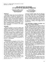
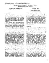
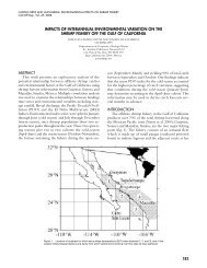
BRODEUR ET AL.: VARIABILITY IN ZOOPLANKTON BIOMASSCalCOFl Rep., Vol. 37, 199670N60504030WINTER 197265N605550454035201 40E 160 180 160 140 120WWINTER 1977N iio ria 150 iio iio iio3025I65N60msn COLUMBIA55504540201140E 160 180 160 140 120W w ti0 Ih 150 li0 ,io 120Figure 2. Winter mean sea-level pressure from Emery and Hamilton (1985) for two contrasting years, and the alternate states of atmospheric and oceanic circulationpatterns in the eastern North Pacific Ocean proposed by Hollowed and Wooster (1992).353025Iinflux of water from the same source-the SubarcticCurrent. We examine physical data relevant to regimeshiftchanges in flow between the Alaska Current andCalifornia Current. Finally, we discuss implications ofregime shifts to higher trophic levels and suggest newhypotheses and further studies that could be undertakento address these hypotheses.DATA SOURCES AND METHODSZooplankton Data SetsZooplankton biomass data from 24 years (1 956-80)of vertical net sampling at Station P were used in ouranalyses (figure 1). Before 1969, sampling was conductedover alternate 6-week periods, but after this time, samplingwas continuous (Fulton 1983). Sampling frequencyvaried from 1 to 29 samples per month over 8 to 12months of the year (Frost 1983). Hauls were mainly doneduring daytime, and all were from 150 m to the surface.Sampling gear was changed from a 0.42-m-diameterNORPAC net to a 0.57-m SCOR net in August 1966,although the mesh size remained the same (0.351 mm).Fulton (1983) estimated that the catching efficiency ofthe SCOR net was 1.5 times greater than the NOR-PAC net, based on a series of intercalibration tows. Buta new estimation based on the original data presentedby Fulton (1983) suggests that the correction factor shouldbe higher, somewhere in the range of 1.6-2.1~, with1.77~ being the most likely value (Waddell and McKmnel1995; Frost, Ware, and Brodeur, unpubl. data), whichis what we used in this analysis.Zooplankton displacement volumes from the centralpart of the CalCOFI grid (lines 77-93) over a longertime frame (1951-94) were provided by Paul Smith(NMFS, SWFC, La Jolla). The gear and maximum hauldepths changed during this period from a bridled l-mdiameterring net fished obliquely to 140 m (1951-68)or to 212 m (1969-78) to an unbridled bongo net fished82

BRODEUR ET At.: VARIABILITY IN ZOOPLANKTON BIOMASSCalCOFl Rep., Vol. 37, 1996down to 212 m (1978-94). An analysis by Ohnian andSmith (1995) has determined that the deeper tows withthe 1-ni net are low by a factor of 1.366 compared withthe shallower 3-m nets and the deep bongo tows withoutbridles, and we adjusted the data accordingly.Since we were interested in advective rather than localproduction processes (Chelton et al. 1982), we trimmedthe data set to include only those stations farther than60 km offshore. We initially aggregated the data in severalways, such as by the northern (north of CalCOFIline SO), middle (line 80 to line 90), and southern (southof line 90) parts of the region, as well as by working withonly the most frequently sampled transects (lines 80 and90). We found, however, that the time series utilizingall the data was highly correlated with alniost all othercombinations of data. Therefore, the CalCOFI data fora given year were combined spatially for all analyses. Inadhtion, the number of missing data points was reduced,though large gaps still existed.Additional zooplankton biomass data from oceanicareas of the Northeast Pacific Ocean besides Station Pexist for two time periods (1956-62 and 1980-89, exceptfor 1986), and are more fully described in Brodeurand Ware (1992). In this analysis, we extended the geographicrange of values to 40"N to include the transitionregion south of the subarctic boundary (Pearcy 1991)for both time periods (see figure 3 for sampling locations).Contour maps of zooplankon biomass (g/l,OOOm3) were generated for both time periods with a rasterbasedGIS program (Compugrid, Geo-spatid Ltd.). Yearlyinterpolated means were computed for each year. Sincethe earlier analysis, an additional 5 years (up to 1994)of data collected by Hokkaido University have becomeavailable. Although there is not enough coverage for thislater period to map the overall distribution of biomass,many of the same transects were sampled each year sothat the interannual variability can be examined. Asbefore, only biomass data collected from 15 June to theend of July and in the same geographic area describedby Brodeur and Ware (1992) were included.Time Series AnalysesWe examined the temporal relationship between theStation P zooplankton data and the offshore CalCOFIdata using tinie series cross-correlation analyses (Box andJenkins 3 976). We investigated monthly, seasonal, andannual lagged relationships. The time series of availabledata for each region shows incomplete temporal overlap,especially for the CalCOFI region, which was intermittentlysampled during the 1970s and 1980s (figure4). The dstribution ofboth the Station P and offshoreCalCOFI zooplankton data was highly skewed, and alog-transformation of the data was performed before thetime-series analysis. In addition, a pronounced seasonal'IOcean Station P111951 ' 1957 1963 ' 1969 ' 1975 ' 1981 ' 1987 ' 19931954 1960 1966 1972 1978 1984 1990CalCOFl offshore831 , , , , , , , , , , , , , , I1951 1957 1963 1969 1975 1981 1987 19931954 1960 1966 1972 1978 1984 1990Figure 4. Log-transformed zooplankton biomass time series for OceanStation P and offshore CalCOFl sampling areas.signal is evident in each region (figure 4). This signalwas removed by calculating a yearly average biomassfor each month and season (spring = March-May; sumnier= June-August; fall = September-November; winter= December-February). Both monthly time seriesexhibited substantial lag-1 autocorrelation, which canresult in spurious cross-correlations (Box and Jenkins1976; Myers et al. 1995). Therefore it was necessary tofilter both series by a process known as prewhitening(sensu Box and Jenluns 1976) before computing the crosscorrelationfunction (CCF) at lagged period$.Ocean Surface Current SimulationsDue to a lack of tinie series of open-ocean currentdata, we used a model developed for the North PacificOcean which provided a continuity of surface mixedlayercurrents through space and time. The OSCURS(Ocean Surface CURrent Simulations) model uses griddeddaily sea-level pressure fields to conipute daily winds,and from them to conipute daily ocean surface currents(Ingraham and Miyahara 1988). The long-termmean geostrophic current vectors computed from existingtemperature and salinity versus depth data are added84

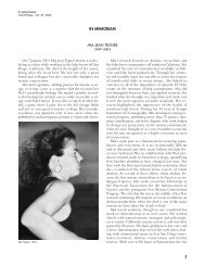
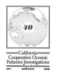
BRODEUR ET AL.: VARIABILITY IN ZOOPLANKTON BIOMASSCalCOFl Rep., Vol. 37, 1996Figure 10. Large-scale distribution of zooplankton biomass from sampling during the 6-week period beginning June 1for 1956-62 and 1980-89. See figure 1 for locations of sampling stations for each period. The insets show the zooplanktonbiomass pixel distributions as a percentage of the total number of pixels for each time period. The overall meanand standard deviation of biomass for the time period are given.87

BRODEUR ET AL.: VARIABILITY IN ZOOPLANKTON BIOMASSCalCOFl Rep., Vol. 37, 1996ANALYSIS OF COVARIATION INSTATION P AND CALCOFI DATA SETSThe magnitude of anonialous values was similar inboth regions, but the CalCOFI data showed an apparentlong-term decline in zooplankton biomass over thelast two decades (figure 4). Autocorrelation plots wereexamined to determine whether serial autocorrelationexists within each region (figure 11). Both monthly timeseries show significant autocorrelation. The CalCOFIdata are significantly autocorrelated up to 12 months, andall correlations up to 24 nionths are positive. Conversely,the Station P data show that anomaly events are muchmore short-lived (lasting 2-3 months), and little teniporalpattern is evident after this time.The cross-correlation between the autocorrelated datasets shows highly significant lagged correlations in bothdirections (figure 12). The presence of autocorrelationwithin both time series, however, renders this relationshiphighly suspect (Katz 1988; Newton 1988). To ascertainwhether there is a real relationship, it is necessaryto prewhiten both series-that is, remove theautocorrelation structure-and then plot the CCF of theresidual series. Both series were adequately described bya lag-1 autoregressive (AR1) model. Separate filters wereused for the two series (“double prewhitening”), and thecoefficients were approximately equal to the lag-1 autocorrelationvalues-0.412 for CalCOFI and 0.524 forStation P. After filtering, alniost all the significant lagcorrelations disappeared (figure 12). The only one thatremained (CalCOFI leading Station P by 2 months) wasquite small (-0.203) and possibly spurious.The effect of prewhitening, while statistically justified,may also have the side effect of overcompensatingfor autocorrelation and removing evidence of an actualsignal. As an alternative to prewhitening, an “effectivedegrees of freedom” is sometimes employed when calculatingthe confidence intervals around the crowcorrelationestiniates (Trenberth 1984). In the case of twoAR1 time series, the true standard deviation at lag 0 isinflated over the no autocorrelation case by.f= [(I + +x*+y)/(1 - +‘y*+y)1°.59where +x and +y are the lag-1 autocorrelation coefficients(Katz 1988). Thus at lag 0, the standard deviationis approximately 1.25 times greater than that cornputedon an assumption of independent data points.i nOcean Station P8 .” , I._95% c. I.c- m ........................................................................??‘0 0.0..............................................................................0-Before prewhitening1 P leads CalCOFl CalCOFl leads P‘J”c 0 ,251._ ............................................................................m-1 .o I2 4 6 8 10 12 14 16 18 20 22 24Lag (months)-.SO] , , p p1 2 1 0 8 6 4 2 0 2 4 6 8 1 0 1 2Lag (months)CalCOFl offshoreAfter prewhitening-c .5-._ 095% c. I.- m................................................m5 0.0-Illillllmrlm I -G .................................................................................0-. O - 1-.5-c .25* s.25..................................................................................-1.01 , , , , , , , , , , , , I2 4 6 8 10 12 14 16 18 20 22 24Lag (months)Figure 11. Serial autocorrelation of Station P and offshore CalCOFl zooplanktonbiomass at various time lags. Upper and lower 95% confidenceintervals are indicated as dashed lines.-.soJ , , , , , , , . , , , , , I12 10 8 6 4 i 0 2 4 6 8 10 i2Lag (months)Figure 12. Cross-correlation between Station P and offshore CalCOFl zooplanktonbiomass at various time lags before and after prewhitening. Theupper and lower 95% confidence intervals are indicated as dashed lines.88

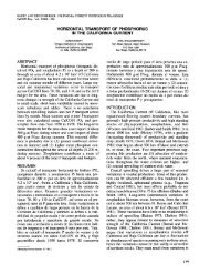
BRODEUR ET AL.: VARIABILITY IN ZOOPLANKTON BIOMASSCalCOFl Rep., Vol. 37, 1996for all years from 1946 to 1994. A substantial divergenceof the tracks occurred in the eastern part of the gulf,with some tracks going north into the Alaska Currentand others heading into shore or turning south. Whenthe tracks are partitioned into pre-1975 and 1975 andlater, some decadal changes become evident (figure 14).In the earlier period, flow into the Alaska Current wasmore relaxed, and a substantial number of the trajectoriesveered southward. The later period appeared to showstronger flow into the Gulf of Alaska, and relatively fewtrajectories went south. The occurrence of either northwardor southward flow tends to run in series of variouslengths (table 3). Simulations started 5" south ofStation P (45"N, 345"W) showed more directed eastwardand southward flow but again showed some differencesbetween the two time periods (figure 15).The model was then used to simulate the north-southdivergence of the Subarctic Current along its easternboundary for equivalent 5-year time periods before andafter the regime shift (1971-75 vs. 1976-80) in order toassess changes in circulation between the two regimes.Long-term mean flow tracks begun in January along145"W showed a more southern diversion before theregime shift than after, with the primary differences inthe trajectories starting at or north of 4S"N (track 5 infigure 16).DISCUSSIONFor oceanic waters of the eastern subarctic PacificOcean, direct evidence for interannual and decadal variationsin biological production-that is, phytoplanktonproduction-is weak. However, zooplankton standingstock, when viewed on a basinwide scale, has varied andseems to be higher since the 1976-77 regime shift.Recognizing that primary production might not havechanged between the regimes, Brodeur and Ware (1992)hypothesized a causal link between increased wind stressand increased zooplankton stock and production, in thatintensified wind mixing would result in deeper mixedlayerdepths (MLD) in winter. This would slow thegrowth rate of the phytoplankton, retard the spring increasein primary production, and allow grazers to makemore efficient use of phytoplankton production. Experimentswith an ecosystem niodel (Frost 1993) do notprovide support for such a mechanism. Indeed, just theopposite effect should occur. A deeper mixed layer inwinter should result in decreased balance between phytoplanktongrowth and grazing in spring, when the surfacelayer restratifies. Phytoplankton production shouldbe less efficiently utilized by grazers, and more productionshould be lost to mixing and sinking below the surfacelayer.But, in fact, there is not much interannual variationin MLD at Station P because of the halocline, and overTABLE 3Yearly Anomalies of Simulated OSCURS Trajectoriesfrom Ocean Station P North or South of the Long-TermMean Trajectory, in Three-Month (Dec.-Feb.)Trajectories for 1946 to 1994North475253575859606263676 9757677787980828385868990919391Souththe observed interannual range of winter MLD (80-130m), Frost's (1993) model suggests that such variationswould have relatively little effect on biological productionor zooplankton biomass at Station P (Frost, unpubl.data). Using a 1-D dynamic mixed-layer model (rnodifiedGanvood model) coupled to a nitrate-phytoplankton-zooplankton(NPZ) model, McClain et al. (1996)found surprisingly little interannual variation in phytoplanktonproduction rate at Station P.464849505154555661646.566687071727374818487889290

BRODEUR ET At.: VARIABILITY IN ZOOPLANKTON BIOMASSCalCOFl Rep., Vol. 37, 199645O40'45'40'Figure 15.Same as figure 14 but with the simulations started 5" south of Station P (45"N, 145'W).92

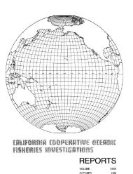
BRODEUR ET AL.: VARIABILITY IN ZOOPLANKTON BIOMASSCalCOFl Rep., Vol. 37, 199660' 50' N 40a140'W1 zoo30'30'Figure 16. Mean simulated flow trajectories for OSCURS model runs for the 5-year period before (upper) and after (lower) the regimeshift. Model runs were started at 145"W on January 1 and run for 12 months. The size of the arrow head and the length of the shaft indicatethe relative current speed. Each trajectory is marked with a circle after 6 months.93

BRODEUR ET AL.: VARIABILITY IN ZOOPLANKTON BIOMASSCalCOFl Rep., Vol. 37, 1996It is likely that events at Station P are not generallyrepresentative of the entire open Gulf of Alaska, dueboth to the singularity of the station and its location.Polovina et al. (1995) reported on interannual changesin winter-spring mixed-layer depth throughout the NorthPacific Ocean. There was considerable spatial variationin change in MLD, with the region of Station P showinglittle long-term change but other areas showing ratherlarge changes (eg, the northeast Gulf of Alaska). Poloviriaet al. (1995) used an NPZ model to look at the effectsof their modeled changes in MLD. The niodel predictsthat large changes in MLD will have little effect on phytoplanktonstock, but potentially large effects on phytoplanktonproduction rate and zooplankton stock inthe mixed layer. Thus, spatial variation in the processescontrolling production rate may explain the apparent increasein zooplankton stock evident on a large spatialscale in the eastern subarctic Pacific Ocean during the1980s. This hypothesis is difficult to test because thereare no basinwide data on nutrient concentrations andbiological observations.To our knowledge, there is no extensive time seriesof phytoplankton standing stock for the CaliforniaCurrent region comparable to the data set from Station€? However, the analysis by Fargion et al. (1993) of CoastalZone Color Scanner data and in situ chlorophyll measurementsindicates little seasonal variation in phytoplanktonstock in the offshore area represented by thezooplankton data presented here (30” to 35”N). Moreover,phytoplankton pigment concentrations are similarto those at Station P (cf. Chavez 1995). Because theCalifornia Current region covered by the zooplanktondata is at considerably lower latitude than Station P, it isprobable that higher phytoplankton production accountsfor the higher zooplankton standing stock observed (figure7).Two factors hinder definitive identification of a lead/lagor “out-of-phase” relationship between zooplanktonproductivity at Station P and the CalCOFI region. First,as noted earlier, there is a great deal of missing data inboth regions. Secondly, the high observed autocorrelation,the robust estimation of which is also hindered bydata gaps, needs to be removed. Despite these difikulties,there is evidence that the two regions are negativelyrelated. It is less clear whether there is a consistent lagtime between the two regions. The evidence points moretoward anomalies at Station P leading anomalies atCalCOFI. It is possible that the inverse relationship isdue to differential (i.e., inverse) flow from the SubarcticCurrent, but that the flow speed within each regime ishighly variable, hence the lack of a consistent lag relationship.El Nifio-Southern Oscillation (ENSO) events areanother factor that may play a role in the timing and in-tensity of anomalous zooplankton production. DuringENSO events. positive SST anomalies are propagatedpoleward in the form of coastally trapped Kelvin waves.Roemmich and McGowan (1995a, b) attributed the declinein CalCOFI region zooplankton biomass to seasurfacewarming, part of which resulted from a largenumber of ENSO events since the mid-1970s. Whilesea-surface temperature anomalies associated with ENSOevents have occurred in the Gulf of Alaska (Wooster andFluharty 1985), as often as not, there has not been anyNorth Pacific Ocean response (Freeland 1990; Baileyet al. 1995). Thus, depending on the magnitude andnorthward extent of the ENSO event and the StationP zooplankton response to surface warming, there is thepotential for a Station P response to lag a CalCOFI response.At the very least, the ENSO factor serves tocloud the relative effects on zooplankton productivityfrom variations in the Subarctic Current.It niay not be coincidental that the increase in zooplanktonshown here in the Subarctic Pacific is oppositeto the trend for California Current zooplankton reportedby Roemmich and McGowan (1 995a, b). Althoughthere is some indirect biological evidence for the oceancirculationmodel proposed by Hollowed and Wooster(1992), the hydrographic evidence is more limited.However, several recent papers shed some light on theissue and suggest considerable modification to the model.Tabata (1991), in reexamining the Chelton and Davis(1982) premise, found a correlation between the coastalcomponent of the Alaska Current and California coastalsea levels, particularly during El Niiio years. He attributedthis correlation, however, to the coastal currentsbeing in phase from Canada to California rather than tochanges in the bifurcation of the Subarctic Current. Kellyet al. (1993) analyzed sea-surface height anomalies forthe Northeast Pacific Ocean over a 2.5-year period. Theirresults tended to support those of Chelton and Davis(1982) that the California and Alaska Current systemsfluctuate “out of phase,” coinciding with variations inwind-stress curl in the North Pacific Ocean and subsequentdiversion of flow from the Alaska Gyre into theCalifornia Current, as well as with some correlation withENSO dynamics. Van Scoy and Druffel (1993), in ananalysis of tritium (‘H) concentrations in seawater fromOcean Station P and a station in the southern CaliforniaCurrent, suggest that there is increased advection of subpolarwater into the California Current during non-ElNifio years and that ventilation of the Alaska Gyre (intensification)occurs during El Nifio years.Lagerloef (1995), in his analysis of dynamic topographyin the Alaska Gyre during 1968-90, suggested thatafter the well-documented climatic regime shift of thelate 1970s, the Alaska Gyre was centered more to the eastand that its circulation appeared weaker after the shift94

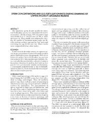
BRODEUR ET AL.: VARIABILITY IN ZOOPLANKTON BIOMASSCalCOFl Rep., Vol. 37, 1996than before. The implication is that the intensificationof the winter Aleutian Low associated with the regimeshift did not result in a spin-up of the Alaska Gyre.Finally, Miller (1996) reviews some recent advancesin large-scale modeling of the California Current andits interaction with basin-scale circulation and forcing.He reports the significant deepening of the thermoclineoff California after the 1976-77 regime shift similar tothat described by Roemrnich and McGowan (1995a)and attributes this to basin-scale changes in wind stresscurl. This is achieved at two time scales-the first at thedecadal and North Pacific Gyre scale, forced by significantdeepening and weakening of the Aleutian Low, andthe second at the interannual ENSO scale, forced bywaves propagating through the ocean from the tropics.Miller (1996) also reported that after the 1976-77 regimeshift there appeared to be a stronger than normal northwardflow into the central Gulf of Alaska but little changein the flow into the California Current system.If zooplankton biomass is advected preferentially toeither region, as the current-simulation model suggests,then this allochthonous biomass should be higher thanthat produced locally for our results to be valid. Thereare few coniparable measurements of zooplankton biomassin both the Transition Doniain and SubarcticDoniain. Our data for the large-scale sampling duringthe 1980s suggest that levels were high in the TransitionDomain and are somewhat higher than in the centralpart of the Alaska Gyre. Data taken in summer for severalyears from north-south transects in the western subarctic(155"E, 170"E, 175.5"E, and 180"E) show elevatedzooplankton wet weights in the transition zonecompared with those in the subarctic (Shiga et al. 1995).Sampling along 180" and in the Gulf of Alaska duringJune and July of 1987 revealed higher zooplankton biomassin transition zone waters than in the central SubarcticDomain, especially in the 150-300-ni depth strata(Kawaniura 1988).An alternative explanation for the inverse relationshipin zooplankton might be that similar large-scale changesin thermal structure of the western North Pacific (Venricket al. 1987; Royer 1989; Roemmich and McGowan1995a; Miller 1996) could have radically different effectson biological production in the two regions. At StationP, the slightly warmer temperature of the mixed layercould directly affect increased zooplankton productionrate and standing stock, as suggested by Conversi andHameed (1996). The same warming and associated deepeningof the upper mixed layer (Miller 1996) could causedecreased zooplankton production and standing stock inthe California Current region by impeding the supplyof nutrients to the surface layer (Roemmich andMcGowan 1995a). Our data are not sufficient to allowexamination of this alternate hypothesis.IMPLICATIONS FOR HIGHER TROPHIC LEVELSThe dramatic increase and change in distribution ofmesozooplankton biomass seen in the subarctic PacificOcean between the periods 195642 and 1980-89 wouldbe expected to have important ramifications for highertrophic levels dependent on these food sources. Brodeurand Ware (1995) documented substantial increases in thecatch rates of most pelagic nekton (fishes, squids, andelasmobranchs) caught in research gill nets over roughlythe same time periods. The only species that showed adecline in catch rates (jack mackerel, Tvachuvus symmetvirus)is primarily a California Current species which migratesinto the Gulf of Alaska only during periods ofpeak abundance. Although these authors were not ableto convert catch rates to abundance or biomass becauseof the paucity of collaborative time series of abundancesfor the noncommercial species, Brodeur and Ware (1 995)estimated that total salmon abundance nearly doubledbetween these two periods.For the present study, we combined catch data ofthe 14 species examined by Brodeur and Ware (1995)and plotted nekton catch-rate distributions for roughlythe same two time periods over the same geographicrange examined previously for zooplankton. Althoughthere are differences between them, the nekton distributionplots (figure 17) showed some similarities to thezooplankton distribution in that most concentrations areoffshore in the Alaska Gyre during the 1950s and occurin a band around the outside of the gyre in the 1980s.The magnitude of the increase in catch rate (figure 17inset) is also similar to that of the plankton. Althoughthis is not cogent evidence of a strong link between thesetrophic levels, since there is often an additional trophiclevel (macrozooplankton and micronekton) between themesozooplankton and the larger nekton, there is enoughcommonality in the distribution patterns to suggest thatthe distribution and abundance of zooplankton is positivelyrelated to that of higher-level predators.Coastal fishes in the Gulf of Alaska would be expectedto benefit most from the increase in zooplankton bioinassthat we observed during the 1980s. High rates ofupwelling in the center of the Alaska Gyre would pushnutrients and subsequent phytoplankton and zooplanktonproduction onto the shelf along the edge of the gulf,thereby stimulating coastal production. Cooney (1986)has suggested that large oceanic species of copepods(Neocalanus spp. and Eircalanus buugii) are transportedonto the shelf in the northern Gulf of Alaska, providingrich food resources for the coastal community. Adirect link between atmospheric circulation, oceaniccopepod production, and sablefish (Anol?lol70n~a-finzbvia)recruitment has been hypothesized by McFarlane andBeamish (1992), but such mechanisms have not beenexplored for other demersal fishes.95

BRODEUR ET AL.: VARIABILITY IN ZOOPLANKTON BIOMASSCalCOFl Rep., Vol. 37, 1996Figure 17. Large-scale catch-rate distribution for 14 species of nekton commonly caught in research gill nets duringthe periods indicated. See Brodeur and Ware (1995) for sampling methodology, locations of sampling stations, andspecies included. Insets show nekton biomass pixel distributions as a percentage of the total number of pixels for eachtime period. The overall mean and standard deviation of biomass for the time periods are given.

BRODEUR ET AL.: VARIABILITY IN ZOOPLANKTON BIOMASSCalCOFl Rep., Vol. 37, 1996For an investigation of ocean effects on fish species,Pacific salmon are an attractive group to study, since theyhave a relatively short life span, show substantial interannualvariability in marine survival, and can be reliablycensused at least several times during their life history.As discussed previously, Pacific salmon stocks have substantiallyincreased in abundance since the mid-1970s inAlaska waters, whereas southern stocks have shown oppositetrends (Pearcy 1992; Beaiiiish 1994; Hare andFrancis 1995). In some cases, the inverse relation betweenstocks in the two domains is striking (Francis andSibley 1991). Our analyses suggest that zooplankton biomassin the subarctic region is inversely related to thatin the California Current region. A conlbination of increasedtransport into the Alaska Current and advectionof nutrients and zooplankton onto the shelf would probablyincrease the carrying capacity for juvenile salmonentering Alaska coastal waters (Cooney 1984).By studying time lags between atmosphere/ocean andsalmon statistics, Francis and Hare (1994) indicated thatthis regime-scale effect on Alaska sahiion production ismost likely to be felt during the early ocean life history.If salmonid production and survival are liniited by factorsoccurring early in their marine life history, then therelative flow into the California Current and AlaskaCurrent may profoundly affect their dynamics by eiihancingprey production for siiiolts in the coastal zone.However, the increasing number of salmon surviving tomaturation in the open ocean after the regime shift mayhave imposed an excess burden upon the oceanic zooplankton,which did not appear to increase as dramaticallyas those in the coastal zone (figure 10). It is likelythat the amount of zooplankton available per individualsalmon has decreased over this period, as suggestedby Peterman (1987), which may be manifested in thelong-term decreases in size at age and the older age ofmaturity witnessed in several salmon stocks (Ishida et al.1993; Helle and Hoffiiian 1995).SUGGESTIONS FOR FURTHER STUDY1. Examine taxonomic composition of zooplanktonover time to see if shifts in species coinposition haveoccurred along with the decadal-scale biomass shifts.This objective has been facilitated by the entry ofthe entire Station P detailed zooplankton data setin digital format that may be amenable to analyses(Waddell and McKinnel 19‘95).2. Construct more spatially-explicit coupled physicaland NPZ models to account for geographic variabilityin ocean condtions, nutrient input, and phytoplanktonand zooplankton species composition(eg, as in McGillicuddy et al. 1995).3. Use models to examine potential top-down controlon phytoplankton and Zooplankton populations,extendng-if possiblesonie of the presently availablemodels (e.g., Frost 1993) to include nekton.Establish new oceanic sampling sites for coniparisonwith Station P to see whether processes occurringat Station P are representative of the subarcticregion as a whole.Continue any present time series sampling, andifpossible-revive discontinued sampling. It is inperativethat the methodology does riot changesubstantially during any time series. If it becomesnecessary to make changes, then at least a sufficientnumber of intercalibration studies between old andnew methodologies should be coiiducted to providea seamless time series.Examine factors that control the production ufphytoplanktonin the open subarctic Pacific. A majoruncertainty concerns the rate of supply of iron,which may stimulate the growth rate of large phytoplanktonspecies, enhance the growth rate oflarge zooplankton, and produce favorable feedingand growth conditions for pelagic fish.ACKNOWLEDGMENTSWe thank Michael Mullin of the Scripps Institutionof Oceanography for inviting us to participate in thesymposium. Paul Smith of the La Jolla NMFS laboratorygenerously provided the CalCOFI data. Earlier draftsof the manuscript were reviewed by Art Kendall andMichael Mullin. This is NOAA’s Fisheries OceanographyCoordiiiated Iiivestigations Contribution FOCI-0273.97

BRODEUR ET AL.: VARIABILITY IN ZOOPLANKTON BIOMASSCalCOFl Rep., Vol. 37, 1996Chelton, D. B. 1984. Short-term climate variability in the Northeast PacificOcean. 61 The influence of ocean conditions on the production of salmonidsin the North Pacific, W. G. I’earcy, ed. Corvallis: Oregon State Univ. SeaGrant Rep. W-83-001, pp. 87-99.Chelton, D. B., and R. E. Davis. 1982. Monthly nieaii sea level variabilityalong the western coast of North America. J. Phy!. Oceaiiog. 12:757-784.Chelton, D. U., 1’. A. Bernal, and J. A. McGowan. 1982. Large-scale interannualphysical aiid biological interaction in the California Current. J. Mar.Kes. 40:1095-1125.Chiversi, A., and S. Hameed. 1996. Quasi-biennial component of zooplanktonbiomass variability in the subarctic Pacific. J. Geophyc. Res.Cooney, K. T. 1984. Some thoughts on the Alaska Coastal Current as afeeding habitat for juvenile salnioii. In The influence of ocean conditionson the production of salmonids in the North Pacific, W. G Pearcy, ed.Corvallis: Oregon State Univ. Sea Grant Rep. W-83-001, pp. 256-268.. 1986. The seasonal occurrence of Riwralaniij crisratio, Seocalanusybnrclinrs, and Eiicalanur 6ro1,qii over the thelf of the northern Gulf of Alaska.Cont. Shelf Res. 5:541-553.Emery, W. J., aiid K. Hamilton. 1985. Atmospheric forcing of interannualvariability in the Northeast Pacific Ocean: connections with El Nirio. J.Geophys. Res. 90:857-868.Fargion, G. S., J. A. McGowan, and R. H. Stewart. 1993. Seasoiiality ofchlorophyll concentrations in the California Current: a comparison of twomethods. Calif. Coop. Ocemic Fish. Invest. Rep. 34:35-50.Fashani, M. J. K. 1995. Variations in the seasonal cycle of biological productionin subarctic oceans: a model sensitivity analysis. Deep-Sea Res.421111-1149.Francis, R. C. 1993. Cliinate change and salnioiiid production in the NorthPacific Ocean. [ti Proceedings of the Ninth Annual Pacific Climate (PA-CLIM) Workshop, K. T. Iiedmond and V. L. Tharp, eds. Calif. Dcp.Water Res. Tech. Rep. 34, pp. 33-43.Francis, R. C. and S. R. Hare. 1994. Ilecadal-scale regime shifts in thelarge marine ecosytenis of the North-east Pacific: a case for historical science.Fish. Oceanog. 3:279-291.Francis, R. C. aiid T. H. Sibley. 1991. Climate change and fisheries: whatare the real issues? NW Eiiviron. J. 7:295-307.Freeland, H. J. 1990. Sea surface temperatures along the coast of BritishCklunibia: regional evidence for a wariiiing trend. Can. J. Fish. Aquat.SCI. 47:346-350.Frost, B. W. 1983. lnterannual variation of zooplankton standing stock inthe open Gulf of Alaska. 117 From year to year: interannual variability ofthe environnient and fisheries of the Gulf ofAlask3 aiid the Eastern HeringSea, W. S. Wooster, ed. Seattle: Washington Sea Grant, pp. 146-157.. 1993. A modelling study of processes regulating plankton standingstock and production in the open rubarctic Pacific Ocean. Prog. Oceanogr.32: 17-56.Fulton, J. 1983. Seasonal and annual variations of net zooplankton at OceanStation “P”, 1956-1980. Can. Ilata Rep. Fish. Aquat. Sci. 374, 65 pp.Grahaiii, N E. 1995. Simulation of recent global temperature trends. Science267:666-671.Hare, S. li., and K. C. Francis. 1995. Cliniate change and salnioii productionin the Northeast Pacific Ocean. 1i1 Climate change and northern fishpopulations, K. Beaiiirh, ed. Can. Spec. Pub. Fish. Aquat. Sci. 121:357372.Helle, J. H., and M. S. Hoffiiian. 1995. Size decline and older age at iiiaturityof two chum salmon (Oncorhyidictr kcfa) xocks in western NorthAmerica, 1972-92. Jii Climate change and northern fish populations, K.Beaiiiish, ed. Can. Spec. Pub. Fish. Aquat. Sci. 121 :245-260.Hollowed, A. B., and W. S. Woo\ter. 1992. Variability ofwinter ocean conditionsand strong year classes of Northeast Pacific groundfish. ICESMar. Sci. Synip. 195:433-444.Hrieh, W. W., arid G. J. Boer. 1992. Global climate change and ocean upwelling.Fish. Ocranogr. 1333-338Ingraham, W. J.,Jr., and R. K. Miyahara. 1988. Ocean surface current \inulationsin the North I’asific Ocean and Benng Sea (OSCURS- NumericalModel). US. Llep. Conimer., NOAA Tech Memo. NMFS F/NWC-130,15.5 pp.Ishida, Y., S. lto, M. Kaeriyama, S. McKinnell, and K. Nagasawa. 1993.Recent changes in age and size of chum salmon (Oricorliyrirhr~s keta) 111the North Pacific Ocesn and possible causes. Can. J. Fish. Aquat. Sci..50: 2Y0-295.Katz, K. W. 1988. Use of cross correlations in the search for teleconnectioiis.J. Climatology 8:241-2.53.Kawatnura, A. 1988. Characteristics of the zooplankton biomass distributionin the standard NORPAC net catches in the North Pacific regon. Bull.Plankton Soc. Jpn. 35:175-177.Kelly, K. A,, Caruso, M. J., and J. A. Austin. 1993. Wind-forced variationin sea surface height in the Northeast Pacific Ocean. J. Phys. Oceanogr.232392-241 I.Lagerloef, G. S. E. 1095. liiterdecadal variation\ in the Alaska Gyre. J. Phys.Oceanogr. 252242-22.58,Martin, J. H., and S. Fitzwater. 1988. Iron deficiency limits phytoplanktongrowth in the Northeast Pacific subarctic. Nature 331:341-343.McAllister, C. 11. 1962. Data record, photosynthesis and chlorophyll measureiiientsat Ocean Weather Station “l’”, July 1959 to November 1961.Fish. Res. Board Can., Manuscript Rep. Ser. (Oceanogr. Limnol.), No.126, 14 pp.McAllistrr, C. D., T R. Parsons, and J. D. H. Strickland. 19.59. Data record,oceanic fertility and productivity tiiea~ureiiients at Ocean Weather Station“P”, July and August lY59. Fish. Res. Board Can., Manuscript Rep. Ser.(Oceanogr. Limnol.), No. 5.5, 31 pp.McClain, C. R., K. Arrigo, K. Tal, arid D. Turk. 1996. Observations andsimulations of physical and biological processes at Ocean Weather StationP, 1951-1980. J. Geophys. Res. 101:3697-3713.McFarlane, G. A,, and R. J. Heaniisli. 1992. Cliiiiatic influence linkiiig copepodproduction with mong year-classes in sablefish, An‘ip~iipo,iiaiii,Ihr?’a.Can. J. Fish. Aquat. Sci. 59743-753.McGillicuddy, 11. J., Jr., A. R. Robinson, and J. J. McCarthy. 1995. Coupledphysical and biologcal modelling ofthe spring bloom in the North Atlantic(11): three diniensioiid bloom and post-bloom processes. Deep-sea Res.421359-1398,Miller, A. J. 1996. Recent advances in California Current modeling: decadaland iiiteratinual thermocline variations. Cali6 Chp. Oceanic Fish. Invest.Rep. 37 (this volunie).Miller, A. J., D. R. Cayan, T. P. Baniett, N. E. Graham, and J. M. Oberhuber.1994. The 1976-77 climate shift of the Pacific Ocean. Oceanography7:21-26.Myers, I

BRODEUR ET AL.: VARIABILITY IN ZOOPLANKTON BIOMASSCalCOFl Rep., Vol. 37, 1996Shiga, N., K. Nuniata, and K. Fujita. 1995. Long-term variations in zooplanktoncommunity and biomass in the Subarctic Pacific transition domain.Mar. Sci. 17:408-414 (in Japanete).Stephens, K. 1964. Data record, productivity measurenients in the NortheastPacific with associated chemical and physical data, 1958-1964. Fish. Res.Board Can., Manuscript Rep. Ser. (Oceanogr. Limnol.) No. 179, 168 pp.. 1966. Data record. Primary production data from the NortheastPacific, January 1964 to December 1965. Fish. Res. Board Can., ManuscriptRep. Ser. (OceanobT. Limnol.) No. 209, 14 pp.. 1968. Data record. Primary production data from the NortheastPacific, January 1966 to Deceniber 1967. Fish. Res. Board Can., ManuscnptRep. Ser. (Oceanogr. Limnol.) No. 957, 58 pp.1977. Primary production data from weatherships occupying OceanStation “P” 1969 to 1975. Fish. Mar. Serv. Data Rep. 38, 88 pp.Tabata, S. 1991. Annual and interannual \wiability of baroclinic transportsacross Line P in the Northeast Pacific Ocean. Deep Sea Res. 38 (Suppl.l):S221-S245.Trenberth, K. E. 1984. Some effects of finite sample size and persistence onmeteorological statistics. Part I: autocorrelations. Man. Weather Kev.112:2359-2368.. 1990. Recent observed interdecadal climate changes in the NorthernHemisphere. Bull. Am. Meteorol. Soc. 71 :988-993.Trenberth, K. E. and J. W. Hurrell. 1994. Decadal atmosphere-ocean variationsin the Pacific. Clim. Dynamics 9:303-319.Van Scoy, K. A,, and E. K. M. Druffel. 1993. Ventilation and transport ofthermocline and intermediate waters in the Northeast Pacific during recentEl Nirios. J. Geophys. Kes. 98:18,083-18,088.Venrick, E. L., J. A. McGowan, D. R. Cayan, and T. L. Hayward. 1987.Climate and chlorophyll a: long-term trends in the central North PacificOcean. Science 238:70&72.Waddell, B. J., and S. McKinnell. 1995. Ocean Station “Papa” detailed zooplanktondata: 1956-1980. Can. Tech. Rep. Fish. Aquat. Sci. 2056, 21 pp.Ware, D. M., and G. A. McFarlane. 1989. Fisheries production domains inthe Northeast Pacific Ocean. In Effects of ocean variability on recruitmentand an evaluation of parameters used in stock assessment models, R. J.Beamish and G. A. McFarlane, eds. Can. Spec. Publ. Fish. Aqudt. Sci.108:359-379.Welschmeyer, N. A., S. Strom, R. Goericke, G. DiTullio, M. Belvin, andW. Petersen. 1993. Primary production in the subarctic Pacific Ocean:Project SUPER. Prog. Oceanogr. 32:lOl-135.Wickett, W. P. 1967. Ekman transport and zooplankton concentration inthe North Pacific Ocean. J. Fish. Res. Board Can. 24:581-594.Wiebe, P. H. 1988. Functional regression equations for zooplankton displacementvolume, wet weight, dry weight, and carbon: a correction. Fish.Bull. U.S. 86:833-835.Wong, C. S., F. A. Whitney, K. Iseki, J. S. Page, and J. Zeng. 1995. Analysisof trends in primary productivity and chlorophyll-a over two decades atOcean Station P (50”N, I45’W) in the Subarctic Northeact Pacific Ocean.In Climate change and northern fish populations, R. Beamish, ed. Can.Spec. Pub. Fish. Aquat. Sci. 121:107-117.Wooster, W. S., and D. L. Fluharty. 1985. El Nifio north. Seattle: WashingtonSea Grant, Univ. Wash., 312 pp.99