Structured Markov chain solver: MATLAB tool extensions

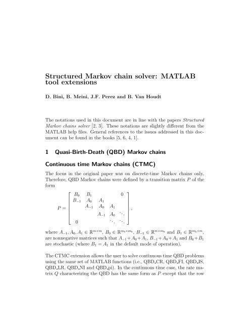
Structured Markov chain solver: MATLABtool extensionsD. Bini, B. Meini, J.F. Perez and B. Van HoudtThe notations used in this document are in line with the papers StructuredMarkov chains solver [2, 3]. These notations are slightly different from theMATLAB help files. General references to the issues addressed in this documentcan be found in the books [5, 6, 4, 1].1 Quasi-Birth-Death (QBD) Markov chainsContinuous time Markov chains (CTMC)The focus in the original paper was on discrete-time Markov chains only.Therefore, QBD Markov chains were defined by a transition matrix P of theform⎡⎤B 0 B 1 0B −1 A 0 A 1P =A −1 A 0 A 1,⎢⎣A −1 A 0.. .⎥⎦.0.. . ..where A −1 , A 0 , A 1 ∈ R m×m , B 0 ∈ R m b×m b, B−1 ∈ R m×m b and B1 ∈ R m b×m ,are nonnegative matrices such that A −1 +A 0 +A 1 , B −1 +A 0 +A 1 and B 0 +B 1are stochastic (where B 1 = A 1 in the default mode of operation).The CTMC extension allows the user to solve continuous time QBD problemsusing the same set of MATLAB functions (i.e., QBD CR, QBD FI, QBD IS,QBD LR, QBD NI and QBD pi). In the continuous time case, the rate matrixQ characterizing the QBD has the same form as P except that the row

2 M/G/1-type Markov chains 2sums of Q equal zero, while P is stochastic. Moreover, the only negativeentries of Q appear on the main diagonal of A 0 and B 0 .In the continuous time case the R, G and U matrices solve the following setof equations:0 = A −1 + A 0 G + A 1 G 2 ,0 = A 1 + RA 0 + R 2 A −1 ,U = A 0 + A 1 (−U) −1 A −1 .(1)Furthermore, one has G = (−U) −1 A −1 , R = A 1 (−U) −1 . When the input isa continuous time QBD, it is automatically transformed to a discrete timeproblem (via a uniformization) such that the ˜G, ˜R and Ũ solution of thediscrete time problem obeys: G = ˜G, R = ˜R and U = λ(Ũ − I) (withλ = max(−diag(A 0 ))). The G, R and U matrix of the continuous time problemare returned as output.If the continuous time QBD is positive recurrent, the following set of equationsholdπ n = π 1 R n−1 ,π 0 B 0 + π 1 B −1 = 0,π 0 B 1 + π 1 (A 0 + RA −1 ) = 0,π 0 e + π 1 (I − R) −1 e = 1,for n > 1. The QBD pi function automatically detects the continuous natureof the problem and will solve it by transforming it to a discrete time problem,having ˜π as a solution, such that ˜π = π.2 M/G/1-type Markov chainsAlternate Shift: ShiftType optionThe computation of the G matrix is accelerated (in the default mode) by theMG1 CR, MG1 NI and MG1 FI functions by applying the shift technique.Assume that A i = 0 for (i > M). The default shift technique (ShiftType =’one’) makes use of the following blocks Ãi, i ≥ −1. If the chain is positive

2 M/G/1-type Markov chains 3recurrent, setà −1 = A −1 (I − Q),à i = A i − ( ∑ ij=−1 A j − I)Q, 0 ≤ i ≤ M,where Q = eu T and u is any vector such that e T u = 1. Otherwise, setà −1 = A −1à 0 = A 0 + EA −1à i = A i − E(I − ∑ i−1j=−1 A j), 1 ≤ i ≤ M,where E = uv T , with u being any nonzero vector, and v such that v T u = 1and v T ( ∑ Mi=−1 A i) = v T .It has been proved that the roots of the polynomials ã(z) = det(λI −∑ Mi=−1 zi+1 à i ), and a(z) = det(λI − ∑ Mi=−1 zi+1 A i ), are the same exceptfor the root z = 1 of a(z) which is shifted to zero or to the infinity for ã(z)according to the recurrent or transient nature of the chain under consideration.We can also accelerate the convergence by shifting the largest root 0 ≤ τ 1, ˆτ ∈ Rto infinity (in the positive recurrent case). Setting the ShiftType = ’tau’,causes this type of shift operation. The τ and ˆτ roots are computed efficientlythrough a bisection algorithm. Whether the ’one’ or ’tau’ shift is themost effective depends on the numerical example at hand.Finally, the double shift (activated by setting the ShiftType option to ’dbl’)combines both the ’one’ and the ’tau’ shift and typically requires the leastnumber of iterations. In the positive recurrent case, the smallest root ˆτ >1, ˆτ ∈ R is first shifted to infinity, afterwards the zero in z = 1 is shifted tozero. In the transient case, we first shift the zero in z = 1 to infinity andnext shift the the largest root 0 ≤ τ < 1, τ ∈ R to zero.Newton iterationThe computation of the matrix G via a Newton iteration is now also supported(via the function MG1 NI) and relies on a fast version of Newton’s

3 GI/M/1-type Markov chains 4iteration for M/G/1-type Markov chains [7]. At each iteration a linear systemof the following form needs to be solvedM+1∑j=1B j XA j−1 = C,where M is the the largest integer such that A M > 0 and m is the block size.Such a system can be solved using a direct sum approach (which happenswhen the option Mode is set to DirectSum), but this results in a time complexityof O(m 6 + m 4 M), as is the case for the Newton iteration discussed in[1]. By relying on a Schur decomposition of A in the linear system above, thetime complexity per iteration can be reduced to O(Mm 4 ). The modes RealSchurand ComplexSchur implement this approach using a real and complexSchur decomposition, respectively. Additionally, each of these modes can alsobe combined with a shift operation, the RealSchurShift mode is the defaultmode for the MG1 NI function.Two more functions: MG1 NI LRA0 and MG1 NI LRAi further exploit potentiallow rank properties of the matrices A i . The MG1 NI LRA0 functionreduces the time complexity per iteration to O(Nm 2 r 2 + m 3 r) when A −1 canbe decomposed as A −1 = Â−1Γ, where Â−1 is of size m × r and Γ of sizer ×m, with r < m. The MG1 NI LRAi function reduces the time complexityper iteration to O(Nm 2 r 2 + Nm 3 ) when A i , for i ≥ 0, can be decomposedas A i = ΓÂi, where Âi is of size r × m and Γ of size m × r.3 GI/M/1-type Markov chainsNew parameter ’Dual’In the first edition of this tool, the R matrix of a GI/M/1-type Markov chainwas computed by computing the G matrix of its Ramaswami dual, fromwhich R can be obtained easily. In the current version of the tool, the usercan select one of two duals: the Ramaswami or Bright dual, by setting the’Dual’ parameter to ’R’ or ’B’, respectively. Setting the ’Dual’ parameterto ’A’ (Automatic) causes the software to select the Bright dual for positiverecurrent chains and the Ramaswami dual for transient ones as this choice is

3 GI/M/1-type Markov chains 5typically the most efficient (for null recurrent chains, both duals are identical).The Ramaswami dual of a GI/M/1-type Markov chain characterized by(A i ) i≥−1 is an M/G/1-type Markov chain characterized by the series of matrices(A (r)i ) i≥−1 withA (r)i = (∆ (r) ) −1 A ′ i(∆ (r) ),for i ≥ −1 and ∆ (r) = diag(π), where π is the stochastic left-invariant vectorof A = ∑ i≥−1 A i.The Bright dual of a GI/M/1-type Markov chain characterized by (A i ) i≥−1 isan M/G/1-type Markov chain characterized by the series of matrices (A (b)i ) i≥0withA (b)i = (∆ (b) ) −1 A ′ i(∆ (b) )τ i ,for i ≥ −1 and ∆ (b) = diag(w), where w is the positive stochastic lefteigenvectorof A(τ) with eigenvalue τ, where A(z) = ∑ ∞i=0 A i−1z i . The scalarτ depends on whether the chain is positive recurrent or transient. In the positiverecurrent case we have: τ = sp(R) < 1 the spectral radius of R, whilein the transient case τ > 1 is the smallest zero of det(zI − A(z)) outside theunit circle.The G matrix of the Ramaswami or Bright dual, denoted as G (r) and G (b)respectively, satisfy the following relation with the R matrix of the originalGI/M/1-type Markov chain:R = (∆ (r) ) −1 (G (r) ) ′ (∆ (r) ) = (∆ (b) ) −1 (G (b) ) ′ (∆ (b) )τ,allowing us to obtain R from the G matrix of its dual.Newton iterationAs for the M/G/1-type Markov chains, a fast Newton iteration is also incorporatedinto the tool. It can be used to compute R by calling the GIM1 Rfunction with the Algor parameter set to NI.

3 GI/M/1-type Markov chains 6The two new functions GIM1 NI LRA0 and GIM1 NI LRAi exploit potentiallow rank properties of the matrices A i . These functions rely on their M/G/1-type counterparts using either the Bright or Ramaswami dual. Notice, inorder to use the GIM1 NI LRAi function the matrices A i must be expressedas ÂiΓ, for i ≥ 0 (as opposed to ΓÂi as in the M/G/1-type case).References[1] D. A. Bini, G. Latouche, and B. Meini. Numerical methods for structuredMarkov chains. Numerical Mathematics and Scientific Computation. OxfordUniversity Press, New York, 2005. Oxford Science Publications.[2] D. A. Bini, B. Meini, S. Steffé, and B. Van Houdt. Structured Markovchains solver: algorithms. In SMCtools Workshop, Pisa, Italy, 2006. ACMPress.[3] D. A. Bini, B. Meini, S. Steffé, and B. Van Houdt. Structured Markovchains solver: software tools. In SMCtools Workshop, Pisa, Italy, 2006.ACM Press.[4] G. Latouche and V. Ramaswami. Introduction to matrix analytic methodsin stochastic modeling. ASA-SIAM Series on Statistics and Applied Probability.Society for Industrial and Applied Mathematics (SIAM), Philadelphia,PA, 1999.[5] M. F. Neuts. Matrix-geometric solutions in stochastic models, volume 2of Johns Hopkins Series in the Mathematical Sciences. Johns HopkinsUniversity Press, Baltimore, Md., 1981. An algorithmic approach.[6] M. F. Neuts. Structured stochastic matrices of M/G/1 type and theirapplications, volume 5 of Probability: Pure and Applied. Marcel DekkerInc., New York, 1989.[7] J. Perez, M. Telek, and B. Van Houdt. A fast Newton’s iteration forM/G/1-type and GI/M/1-type Markov chains. Submitted, 2011.