The New Silicon Strip Detectors for the CMS Tracker ... - HEPHY

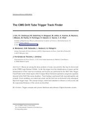
DissertationThe New Silicon Strip Detectors for the CMSTracker Upgradeausgeführt zum Zwecke der Erlangung des akademischen Grades eines Doktors dertechnischen Wissenschaften unter der Leitung vonUniv.Doz. Dipl.-Ing. Dr. techn. Manfred KRAMMERInstitut für Hochenergiephysikder Österreichischen Akademie der WissenschaftenundAtominstitut der Österreichischen Universitäteneingereicht an der Technischen Universität WienFakultät für PhysikvonDipl.-Ing. Marko DragicevicMatrikelnummer: 9627193Mittersteig 2A/DG11040 WienWien, am 21. Dezember 2010

KurzfassungIm einleitenden Teil der Arbeit werden zuerst die wichtigsten Grundkonzepte des CMS Experimentsbeschrieben.Die Aufgaben der einzelnen Detektorsysteme werden erklärt sowie deren technischeRealisierung in CMS.Um die Funktionsweise von Silizium Streifensensoren zu verstehen, werden die dafür wichtigstenGrundlagen der Halbleitertechnologie, insbesondere von Silizium, besprochen. Die notwendigenProzessschritte zur Herstellung von Streifensensoren im sogenannten Planarprozess werden ausführlichbeschrieben. Anschließend werden die möglichen Auswirkungen von Strahlenschäden aufdie Funktion der Sensoren diskutiert.Als Abschluss des allgemeinen Teils, wird das Design der Silizium Streifensensoren des CMSTrackers genauer beschrieben. Die Wahl des Grundmaterials sowie die komplexe Geometrie derSensoren werden eingehend besprochen. Weiters werden die Massnahmen zur Qualitätssicherungwährend der Herstellung der Sensoren diskutiert, sowie das Design und die Konstruktion der Detektormodule.Im Kernteil der Arbeit werden zunächst die Anforderungen an den Spurdetektor diskutiert, diedurch eine Erhöhung der Designluminosität des LHC Beschleunigers (sLHC) bedingt sind. DiesesKapitel motiviert die von mir durchgeführten Arbeiten und erklärt warum die von mir vorgeschlagenenLösungen einen wichtigen Beitrag zur Entwicklung des CMS Tracker Upgrades darstellen.In den folgenden Kapitel werden jene Konzepte präsentiert, die den Betrieb von Silizium Streifensensorenbei sLHC Luminositäten ermöglichen, sowie einige weitere Verbesserungen beim Bau undder Qualitätssicherung der Sensoren und Detektormodule. Die wichtigsten Konzepte und Arbeitensind:• Entwicklung eines Software-Frameworks zum schnellen und flexiblen Design von Teststrukturenund Sensoren.• Auswahl geeigneter Sensormaterialien, welche ausreichend Strahlenresistent sind.• Design, Implementation und Herstellung eines Sets von Teststrukturen zur Qualitätssicherungvon strahlenharten Sensoren und möglichen zukünftigen Entwicklungen.• Elektrische Charakterisierung der Teststrukturen und Analyse der gewonnen Daten.• Design, Implementation und Herstellung von Sensoren mit integriertem Routing der Sensorstreifenzur Ausleseelektronik.• Elektrische Charakterisierung der Sensoren und Analyse der gewonnen Daten.• Funktionstests der integrierten Sensoren in einem Teststrahl Experiment.

• Analyse der gewonnen Daten des Teststrahl Experiments.Alle verwendeten Sensoren und ein Teil der Teststrukturen wurden von mir entworfen und mittelsvon mir entwickelter Werkzeugen implementiert. Der Herstellungsprozess der Sensoren und Teststrukturenwurde in enger Zusammenarbeit mit dem Hersteller von mir konzipiert und begleitet.Weiters wurde die notwendige Analyse der Daten unter meiner Leitung durchgeführt und die Ergebnissein dieser Arbeit erstmals präsentiert.iv

AbstractThe first introductory part of the thesis describes the concept of the CMS experiment. The tasks ofthe various detector systems and their technical implementations in CMS are explained.To facilitate the understanding of the basic principles of silicon strip sensors, the subsequent chapterdiscusses the fundamentals in semiconductor technology, with particular emphasis on silicon. Thenecessary process steps to manufacture strip sensors in a so-called planar process are described indetail. Furthermore, the effects of irradiation on silicon strip sensors are discussed.To conclude the introductory part of the thesis, the design of the silicon strip sensors of the CMSTracker are described in detail. The choice of the substrate material and the complex geometry of thesensors are reviewed and the quality assurance procedures for the production of the sensors are presented.Furthermore the design of the detector modules are described.The main part of this thesis starts with a discussion on the demands on the tracker caused by theincrease in luminosity which is proposed as an upgrade to the LHC accelerator (sLHC). This chaptermotivates the work I have conducted and clarifies why the solutions proposed by myself areimportant contributions to the upgrade of the CMS tracker.The following chapters present the concepts that are necessary to operate the silicon strip sensorsat sLHC luminosities and additional improvements to the construction and quality assurance of thesensors and the detector modules. The most important concepts and works presented in chapters 7to 9 are:• Development of a software framework to enable the flexible and quick design of test structuresand sensors.• Selecting a suitable sensor material which is sufficiently radiation hard.• Design, implementation and production of a standard set of test structures to enable the qualityassurance of such sensors and any future developments.• Electrical characterisation of the test structures and analysis of the measurements.• Design, implementation and production of sensors with integrated routing of signals from thesensor strip to the readout electronics.• Electrical characterisation of the sensors and analysis of the measurements.• Operational tests of the integrated sensors in a test beam experiment.• Analysis of the data recorded during the test beam experiment.

All the sensors and a part of the test structures were solely designed by me and implemented usingtools which were created by myself as well. The manufacturing process for the sensors and teststructures was implemented in close collaboration with the manufacturer. Furthermore, the necessaryanalysis of the data was supervised by me and the results are presented in this thesis for thefirst time.vi

ContentsI. Theoretical and Technical Background Information 11. The CMS Experiment 51.1. Tracking System . . . . . . . . . . . . . . . . . . . . . . . . . . . . . . . . . . . 81.1.1. Pixel Tracker . . . . . . . . . . . . . . . . . . . . . . . . . . . . . . . . . 91.1.2. Strip Tracker . . . . . . . . . . . . . . . . . . . . . . . . . . . . . . . . . 101.2. Calorimeter System . . . . . . . . . . . . . . . . . . . . . . . . . . . . . . . . . . 111.2.1. Electromagnetic Calorimeter . . . . . . . . . . . . . . . . . . . . . . . . . 111.2.2. Hadronic Calorimeter . . . . . . . . . . . . . . . . . . . . . . . . . . . . . 121.3. Muon System . . . . . . . . . . . . . . . . . . . . . . . . . . . . . . . . . . . . . 131.4. Trigger System . . . . . . . . . . . . . . . . . . . . . . . . . . . . . . . . . . . . 142. Basics on Silicon Semiconductor Technology 172.1. Intrinsic Properties of Silicon . . . . . . . . . . . . . . . . . . . . . . . . . . . . . 182.2. Extrinsic Properties of Doped Silicon . . . . . . . . . . . . . . . . . . . . . . . . 212.3. Carrier Transport . . . . . . . . . . . . . . . . . . . . . . . . . . . . . . . . . . . 242.3.1. Drift . . . . . . . . . . . . . . . . . . . . . . . . . . . . . . . . . . . . . . 252.3.2. Diffusion . . . . . . . . . . . . . . . . . . . . . . . . . . . . . . . . . . . 252.4. Carrier Generation and Recombination . . . . . . . . . . . . . . . . . . . . . . . . 262.4.1. Thermal Generation . . . . . . . . . . . . . . . . . . . . . . . . . . . . . 262.4.2. Generation by Electromagnetic Excitation . . . . . . . . . . . . . . . . . . 272.4.3. Generation by Charged Particles . . . . . . . . . . . . . . . . . . . . . . . 272.4.4. Charge Carrier Lifetime . . . . . . . . . . . . . . . . . . . . . . . . . . . 292.5. Basic Semiconductor Structures . . . . . . . . . . . . . . . . . . . . . . . . . . . 312.5.1. The p-n Junction or Diode . . . . . . . . . . . . . . . . . . . . . . . . . . 312.5.2. The n+-n or p+-p Junction . . . . . . . . . . . . . . . . . . . . . . . . . . 372.5.3. The Metal - Semiconductor Contact . . . . . . . . . . . . . . . . . . . . . 382.5.4. The Metal - Oxide - Semiconductor Structure . . . . . . . . . . . . . . . . 382.5.5. The Polysilicon Resistor . . . . . . . . . . . . . . . . . . . . . . . . . . . 452.6. Radiation Damage and the NIEL hypothesis . . . . . . . . . . . . . . . . . . . . . 452.6.1. Bulk and Surface Damage . . . . . . . . . . . . . . . . . . . . . . . . . . 472.6.2. Changes in Properties due to Defect Complexes . . . . . . . . . . . . . . . 482.6.3. Annealing . . . . . . . . . . . . . . . . . . . . . . . . . . . . . . . . . . . 502.6.4. Reverse Annealing . . . . . . . . . . . . . . . . . . . . . . . . . . . . . . 513. Silicon Strip Sensors 533.1. Working Principle . . . . . . . . . . . . . . . . . . . . . . . . . . . . . . . . . . . 53vii

Contents3.2. Design Basics of a Silicon Strip Sensor . . . . . . . . . . . . . . . . . . . . . . . 563.2.1. Strip Geometry . . . . . . . . . . . . . . . . . . . . . . . . . . . . . . . . 563.2.2. DC to AC coupled Strips . . . . . . . . . . . . . . . . . . . . . . . . . . . 573.2.3. Biasing of the Strips . . . . . . . . . . . . . . . . . . . . . . . . . . . . . 583.2.4. Breakdown Protection . . . . . . . . . . . . . . . . . . . . . . . . . . . . 593.2.5. Contact Pads . . . . . . . . . . . . . . . . . . . . . . . . . . . . . . . . . 613.3. Manufacturing of Silicon Sensors . . . . . . . . . . . . . . . . . . . . . . . . . . 633.3.1. Silicon for Silicon Sensors . . . . . . . . . . . . . . . . . . . . . . . . . . 633.3.2. General Process Steps in Planar Technology . . . . . . . . . . . . . . . . . 653.3.3. A Showcase Process Sequence . . . . . . . . . . . . . . . . . . . . . . . . 704. The CMS Silicon Strip Sensors 794.1. Sensor Design . . . . . . . . . . . . . . . . . . . . . . . . . . . . . . . . . . . . . 794.1.1. Choice of Bulk Material . . . . . . . . . . . . . . . . . . . . . . . . . . . 794.1.2. Sensor Geometry . . . . . . . . . . . . . . . . . . . . . . . . . . . . . . . 814.1.3. Strip Geometry . . . . . . . . . . . . . . . . . . . . . . . . . . . . . . . . 814.2. Sensor Quality Assurance . . . . . . . . . . . . . . . . . . . . . . . . . . . . . . . 824.3. Detector Module Design . . . . . . . . . . . . . . . . . . . . . . . . . . . . . . . 83II. Sensor Design for the new CMS Tracker 855. Super LHC and the CMS Upgrade 895.1. Super LHC: a luminosity upgrade . . . . . . . . . . . . . . . . . . . . . . . . . . 895.2. Challenges for the Strip Tracker . . . . . . . . . . . . . . . . . . . . . . . . . . . 935.2.1. Increase in granularity . . . . . . . . . . . . . . . . . . . . . . . . . . . . 935.2.2. Increase in Radiation . . . . . . . . . . . . . . . . . . . . . . . . . . . . . 965.2.3. Tracking Trigger . . . . . . . . . . . . . . . . . . . . . . . . . . . . . . . 985.3. Summary . . . . . . . . . . . . . . . . . . . . . . . . . . . . . . . . . . . . . . . 996. New Bulk Materials and Process Technologies 1016.1. Combined Results from RD50 . . . . . . . . . . . . . . . . . . . . . . . . . . . . 1016.1.1. Full Depletion Voltage and Effective Doping Concentration . . . . . . . . 1036.1.2. Charge Collection Efficiency . . . . . . . . . . . . . . . . . . . . . . . . . 1066.1.3. Reverse Bias Current . . . . . . . . . . . . . . . . . . . . . . . . . . . . . 1076.1.4. Charge Multiplication in Silicon . . . . . . . . . . . . . . . . . . . . . . . 1086.2. Summary . . . . . . . . . . . . . . . . . . . . . . . . . . . . . . . . . . . . . . . 1106.3. Outlook . . . . . . . . . . . . . . . . . . . . . . . . . . . . . . . . . . . . . . . . 1117. SiDDaTA - Silicon Detector Design and Teststructures using AMPLE 1137.1. Motivation for SiDDaTA . . . . . . . . . . . . . . . . . . . . . . . . . . . . . . . 1137.2. Software Architecture . . . . . . . . . . . . . . . . . . . . . . . . . . . . . . . . . 1147.2.1. Integration of SiDDaTA . . . . . . . . . . . . . . . . . . . . . . . . . . . 1157.2.2. Defining a Device . . . . . . . . . . . . . . . . . . . . . . . . . . . . . . 1157.3. Design Guidelines . . . . . . . . . . . . . . . . . . . . . . . . . . . . . . . . . . . 1177.3.1. Directory Structure of the AMPLE Code . . . . . . . . . . . . . . . . . . 1177.4. Applications for SiDDaTA . . . . . . . . . . . . . . . . . . . . . . . . . . . . . . 1197.4.1. Collaborations with IFCA Santander and CNM Barcelona . . . . . . . . . 119viii

Part I.Theoretical and Technical BackgroundInformation

IntroductionTo understand the work performed for this thesis and to put the developments in silicon strip technologyinto perspective, it is important to review the basic principles of semiconductor theory andthe current technological status of silicon strip sensors.The first part of this thesis starts with an overview of the CMS experiment and its detector systems.The second chapter provides an in-depth review on semiconductor theory, focusing on topics whichare relevant to understand sensors for ionizing radiation. The following third chapter explains thegeneral layout and the manufacturing technology of standard silicon strip sensors and is concludedby an in-depth description of the sensors and detector modules designed for and operated within thetracking system of the CMS experiment.3

The Compact Muon Solenoid (CMS) experiment is one of two large generalpurposeparticle physics detectors built on the proton-proton Large Hadron Collider(LHC) at CERN in Switzerland and France. Approximately 3,600 peoplefrom 183 scientific institutes, representing 38 countries form the CMS collaborationwho built and now operate the detector. It is located in an undergroundcavern at Cessy in France, just across the border from Geneva.Wikipedia on Compact Muon Solenoid1The CMS ExperimentThe Compact Muon Solenoid (CMS) is one of the four large experiments at the Large HadronCollider (LHC). Similar to the ATLAS experiment[1], it was designed as a multi-purpose discoverydetector assigned to tackle many of todays unanswered questions where the answers are5

1. The CMS Experimentaccessible by the LHC for the first time. The main topics which drove the design choices of theCMS experiment are:• Search for the Higgs Boson• Search for supersymmetric particles• Search for new massive vector bosons• Search for extra dimensions• Standard model measurements• Heavy ion physicsTo exhibit adequate performance on the mentioned activities, the requirements of the CMS detectorcan be summarised as follows:• Good muon identification and momentum resolution over a wide range of momenta in theregion |η| < 2.5, good dimuon mass resolution (≈ 1% at 100 GeV/c 2 ), and the ability todetermine unambiguously the charge of muons with p < 1 TeV/c.• Good charged particle momentum resolution and reconstruction efficiency in the inner tracker.Efficient triggering and offline tagging of τ’s and b-jets, requiring pixel detectors close to theinteraction region.• Good electromagnetic energy resolution, good diphoton and dielectron mass resolution (≈1% at 100 GeV/c 2 ), wide geometric coverage (|η| < 2.5), measurement of the direction ofphotons and/or correct localization of the primary interaction vertex, π 0 rejection and efficientphoton and lepton isolation at high luminosities.• Good ETmiss and dijet mass resolution, requiring hadron calorimeters with a large hermeticgeometric coverage (|η| < 5) and with fine lateral segmentation (∆η × ∆φ < 0.1 × 0.1).These requirements led to the some of the outstanding features of the CMS detector concept, like thehigh-field superconducting solenoid, the all silicon tracker and the fully active scintillating crystalelectromagnetic calorimeter.As most collider experiments, the general design of CMS resembles a barrel shaped onion: severalcylindrical detector layers with discs covering both ends as seen in figure 1.1. The layeredapproach enables particles to be measured and identified using specialised detector systems at eachof the layers. Although concentric spheres would be the optimal geometry, giving the most homogeneouscoverage, it is technically not feasible. Therefore the barrel-like shape proves to be the bestcompromise.Figure 1.2 illustrates the path of the most important particles types when they traverse the detector.The task of the innermost detector system is to determine the particle’s origin (vertex) andto measure the precise track of the particle, hence the name tracker. Thanks to the high magneticfield inside the tracker volume, the curvature of the particle tracks indicate the momentumand the sign of the electric charge of the incident particle. The calorimeters are measuring thekinetic energy of the particles and they are fully hermetic with only muons and neutrinos being6

Figure 1.1.: 3D-view of the CMS experiment showing the location of the detector systems.7

1. The CMS Experimentable to pass through. The superconducting coil creates the magnetic field needed for the trackingsystem and the muon chambers for momentum measurement. The iron return yoke shapesthe field in the outer part of the detector, where muon chambers determine the curved tracks ofmuons.Figure 1.2.: Slice of the CMS detector showing the signals that different particles are inducing in the individual detectorsystems.The CMS detector is 22 m long, has a diameter of 15m and a mass of 12,500 tons. Compared tothe Eiffel Tower in Paris which has a total mass of 10,000 tons, the CMS experiment is a rathercompact structure, hence the term compact in its name.1.1. Tracking System8

1.1. Tracking SystemThe first detector that particles are traversing is the full silicon tracking system. It consists of twodifferent technologies, a pixel tracker and a strip tracker. While both give precise spatial informationon particle tracks, they are optimised to satisfy slightly different demands[2].1.1.1. Pixel TrackerThe pixel or vertex tracker is the innermost detector of CMS covering a mean radii of 4.4 cm to10.2 cm from the beam pipe. Being so close to the interaction point exposes the detector and itsaccompanying electronics to high irradiation as seen in figure 1.3.Fluence (cm -2 )Fluence (cm -2 )Dose (Gy)R=4.3 cmR=7.1 cm10 15 0 10 20 30R=4.3 cmR=7.1 cmR=11 cm10 14 0 10 20 30Pixel BarrelAbsorbed dose10 6 0 10 20 30R=4.3 cmR=11 cmR=7.1 cmR=11 cmPixel BarrelCh. hadron & K0 fluencePixel BarrelNeutron fluence (E>100 keV)10 5z (cm)z (cm)z (cm)! z=32.5 cm" z=46.5 cm! z=32.5 cm" z=46.5 cmPixel EndcapAbsorbed dose! z=32.5 cm" z=46.5 cm10 6 10 1510 15 10 1510 14 10 15Pixel EndcapCh. hadron & K0 fluencer (cm)Pixel EndcapNeutron fluence (E>100 keV)r (cm)10 5r (cm)Figure 1.3.: Simulation results of the energy-integrated charged hadron and neutron fluences and absorbed dose in thepixel detector. All values are for an integrated luminosity of 5 × 10 5 pb −1 [2].While having to cope with the high fluences, the pixel tracker should provide precise vertex positionin the order of 10-20 µm. This is achieved by using silicon pixel sensors with 100 µm× 150 µm pixelsand the ReadOut Chip (ROC) directly bump bonded onto it (see figure 1.4).9

1. The CMS ExperimentFigure 1.4.: Illustration of the CMS pixel sensor and thereadout chip, which is directly bump bondedonto the sensor.Figure 1.5.: The layout of the pixel detector with its barreland endcap regions.These detector modules are integrated into larger support structures. The full detector consists ofthree barrel layers with a total of 768 modules and four forward or endcap disks with a total of 672modules (see figure 1.5). This results in over 65 million readout channels.1.1.2. Strip TrackerThe Silicon Strip Tracker (SST) covers the mean radii from 20 cm to 110 cm. It comprises 15.148detector modules with 24,244 silicon strip sensors each with 512 or 768 strips. This amounts toa total of 9,316,352 readout channels or a silicon area of 206 m 2 and makes it the largest silicondevice today (2010).The SST is divided into four sub detectors, called the Tracker Inner Barrel (TIB), the Tracker OuterBarrel (TOB), the Tracker EndCaps (TEC) and the Tracker Inner Disks (TID).The TIB covers the radii from 20 cm to 64 cm with four layers using sensors with a thickness of 320µm and a strip pitch of 80 µm to 120 µm. The first two layers provide measurements in r − φ andr −z simultaneously using two modules which are mounted back to back where one of the moduleshas a slightly rotated sensor (stereo module). The TOB consists of six layers and covers the radiiup to 110 cm. Its sensors are 500 µm thick with a pitch of 120 to 180 µm . The thicker sensorsshould ensure a good signal-to-noise ratio as each module contains two daisy-chained sensors andtherefore longer strips which exhibit higher noise. Again, the first two layers are equipped withstereo modules. The endcaps are divided into the smaller TID which covers the ends of the TIBand the TEC which extends to fully cover both ends of the tracker. The TID consists of 3 smalldisks with 3 rings of modules where the first two rings are again equipped with stereo modules.The two TECs are composed of 9 disks where each disk needs 12 different types of modules tofully cover the circular shaped area. The rings one, two and five are again equipped with stereomodules.The full tracker provides coverage up to |η| < 2.4 while giving a minimum of 5 hits per track (seefigure 1.6.10

1.2. Calorimeter SystemFigure 1.6.: Layout of the CMS tracker. This two-dimensional view is rotationally symmetric with respect to the beamrunning horizontally through the center. Each single line represents a sensor plane. Layers equipped withstereo modules and therefore providing two-dimensional hit coordinates, are easily spotted by two parallellines close together.1.2. Calorimeter SystemThe calorimeter systems measure the energy of the incident particles by fully stopping them in adense material and measuring the deposited energy. The CMS detectors uses two different kinds ofcalorimeters, as it is common for most collider experiments - an electromagnetic calorimeter and ahadronic calorimeter. The former is placed immediately after the tracking system while the lattersurrounds the electromagnetic calorimeter.1.2.1. Electromagnetic CalorimeterThe Electromagnetic CALorimeter (ECAL) measures the energy of particles which are mainlyinteracting by the electromagnetic force like electrons, positrons and photons. It is a hermetic and11

1. The CMS Experimenthomogeneous calorimeter made of more than 61,000 lead tungsten crystals (PbWO 4 ) in the barrelpart and a further 14,648 crystals in the two endcaps[3].Particles entering the crystals produce scintillating light by electromagnetic interaction. The leadtungsten crystals have excellent properties in terms of short radiation length (X 0 = 0.80 cm) andsmall Moliere radius (R M = 2.2 cm), the light emittance is fast (80% within 25 ns) and the materialis radiation hard. On the downside, the light yield is low (about 30 γ/MeV) which requires highlysensitive photodetectors.To reliably detect the small amount of scintillating light produced inside the crystal, photodetectorswith high intrinsic gain are used. The barrel section uses Avalanche Photo Diodes (APD) while inthe forward parts Vacuum PhotoTriodes (VPT) provide the light measurement.1.2.2. Hadronic CalorimeterIn contrast to the electronic calorimeter, the Hadronic CALorimeter (HCAL) measures the energyof the incident particle using strong interaction. CMS uses a sampling calorimeter, where platesof brass are used as absorber material interleaved with plastic scintillator as the active detectormaterial[4].A particle entering the hadronic calorimeter will interact with the nucleus of the absorber materialcreating hadronic showers. The particles in the shower will induce light in the plastic scintillatorswhich is then transported by wavelength-shifting fibres to multi-channel Hybrid PhotoDiodes(HPD). The HPDs convert photons to electrons and direct them onto silicon sensors where thesephotoelectrons are detected.Most of the HCAL material is inside the magnetic coil to minimize the non-Gaussian tails in the energyresolution and to provide a good containment and hermeticity for the measurement of the missingenergy (ETmiss ). Only a small additional layer of scintillators, the Outer Hadron (HO) calorimeter,is placed beyond the magnet, lining the outside of the vacuum vessel to catch the tails still leakingthrough the calorimeters. This increases the effective thickness of the HCAL to over 10 interactionlengths.12

1.3. Muon SystemCoverage for pseudorapidities of 3 < |η| < 5 is maintained by the Hadron Forward (HF) calorimeter.Its main objective is to improve the measurement of the missing transverse energy and and toenable identification and reconstruction of very forward jets. As the available space in the forwardregion is much more cramped, the design had to be slightly different. To produce shorter andnarrower showers the HF uses steel plates as absorbers and Cherenkov light emitted by quartzfibres embedded in the absorber plates as active detector element. The light is then transferred tophotomultipliers for signal amplification and measurement.1.3. Muon SystemAs the calorimeters are fully hermetic to hadrons and most leptons, the only particles that need to bemeasured past the HCAL are the muons. The muon systems should increase the momentum resolutionfor high momentum muons and provide fast information to the trigger. To achieve these tasks,three types of gaseous detectors are used for the measurement of muons[5].Cathode Strip Chambers (CSC) are used in the endcaps, as the neutron background, the muon rateand the residual magnetic field is high in this region. For the barrel region, where the requirementsare much lower, Drift Tube (DT) chambers are used. Both regions also employ ResistivePlate Chambers (RPC) to provide good timing resolution to identify the correct bunch crossing.The CSCs consist of arrays of positively charged anode wires and and negatively charged cathodestrips made from copper. The wires and strips are perpendicular and embedded in a gas volume.Muons, or any charged particle, ionize the gas and the electrons will move towards the anode wirewhile the ions will drift to the cathode strips. This gives spatial information in two coordinates foreach passing muon and, because of the fast response of the closely space wires, the CSCs are alsoproviding information to the trigger.A 4 cm tube filled with a mixture of argon and CO 2 gas and a thin stretched wire placed along thecenter of the tube, are the basic components of the DTs. Electrons created by ionization from anincident particle drift towards the thin wire where they are registered. By calculating the distanceof the ionization to the wire and the location of the induced signal along the wire, the DTs providetwo coordinates for the position of the incident muon.13

1. The CMS ExperimentThe RPCs can provide a high timing resolution in the order of nanoseconds. They consist of twoparallel plates which are separated by a gas volume. These plates are made of a high resistiveplastic material and are used as positively charged anode and negatively charged cathode. Theelectric field between the plates accelerates the electrons and ions created by ionizing particlestowards the respective electrodes. The full charge created by the incident muon is collected by ametallisation at the backside of the plastic electrodes. As one of the metallisations is patterned intostrips, the RPCs provides a spatial measurement which is used to estimate the muon momentum forthe trigger.1.4. Trigger SystemThe LHC provides collisions every 25 ns or at 40 MHz 1 where the full detector information ofa single event amounts to approximately 1 MB. This would yield a sustained data rate of 40TB/s which is not feasible to write to a storage system in terms of transfer speed and data capacity.Most of the interactions do not involve any new physics processes, as the interaction cross-sectionsfor interesting processes are rather small. Such events which show only well known physics canbe discarded, leaving only those events for storage which might exhibit new physics. Nevertheless,this decision has to be made within a very small timeframe and at the high rate at which the LHCdelivers the events.The CMS experiment choose to implement a two level trigger system with a fully hardware implementedLevel-1 trigger (L1) and an online filter system implemented in software running on aprocessor farm which is called High Level Trigger (HLT)[6].The decision of the L1 trigger, whether to keep an event or discard it, is based on the presenceof certain trigger primitives such as photons, electrons, muons and jets above certain E T and p Tthresholds. This information is collected from the fast detectors in the calorimeters and the muonsystems and only if the event is accepted by the L1, the complete detector information is read out andpassed to the HLT. The L1 has a small time frame of 3.2 µs to make its decision which is based onthe size of the buffers in the front-end electronics inside the detector . This timeframe is reduced bythe transit time of the detector signals from the front-end electronics inside the detector to the servicecavern housing the L1 trigger logic and the return back to initiate the readout of the full detector. Theremaining time allocated for the L1 decision is less than 1 µs! To reach the required performance,while still retaining a high level of flexibility of the used algorithms, the L1 trigger logic is mainlyimplemented in Field Programmable Gate Arrays (FPGA). The achieved data reduction factor is inthe order of 1:10 3 resulting in a L1 data rate of 100 kHz.The HLT is implemented in software where an identical instance of the algorithms is run on severalthousands of CPU cores of a computer farm. For each event accepted by the L1 trigger, the full1 This is not entirely correct, as not all possible bunch locations inside he accelerator are filled. Certain locations are leftvacant to allow the beam dump system enough time to ramp up the extraction magnets and safely extract the beam.Therefore the average collision rate is somewhat lower than 40 MHz.14

1.4. Trigger Systemdetector information is passed to a processor of the HLT. A fast reconstruction of the event, similarto the full offline analysis but with less accuracy, is made to decide whether the event will be storedon disc or discarded.15

Silicon, (Latin: silicium) is the most common metalloid. It is a chemical element,which has the symbol Si and atomic number 14. The atomic mass is28.0855. A tetravalent metalloid, silicon is less reactive than its chemical analogcarbon. As the eighth most common element in the universe by mass, siliconvery rarely occurs as the pure free element in nature, but is more widelydistributed in dusts, planetoids and planets as various forms of silicon dioxide(silica) or silicates. On Earth, silicon is the second most abundant element (afteroxygen) in the crust, making up 25.7% of the crust by mass.Wikipedia on Silicon2Basics on Silicon Semiconductor TechnologyMost modern high energy physics experiments use silicon strip sensors for tracking the trajectoriesof charged particles. Such detectors can be built with a very moderate material budget, offering precisespatial resolution and robust performance even after high irradiation. Costs can be kept withinreasonable amounts, as the production technology of the sensors follows common processes developedin the IC industry. The following chapters review the basic fundamentals needed to understandthe operation of such sensors and how they are manufactured.17

2. Basics on Silicon Semiconductor Technology2.1. Intrinsic Properties of SiliconSilicon is the 14th element in the periodic table of elements and belongs to group IV. It hasfour covalently bound electrons and forms a face-centered cubic structure with a lattice spacingof 5.430710 Å (0.5430710 nm) which is shown in figure 2.1. The most important propertiesof silicon are noted in table 2.1. To comprehend the chemical and electronic properties ofsolid silicon, it is important to understand the energy band structure of solids as seen in figure2.2Figure 2.1.: The face-centered cubic structure of silicon which is the same as for diamond.Substance Si Ge GeAs Diamondlattice diamond diamond zinc blende diamondatomic number 5.4307 5.657 5.653 3.5668average atomic mass 14 32 31+33 6density [g/cm 3 ] 2.329 5.323 5.317 3.515melting point [°C] 1415 937 1238 3907thermal expansion coefficient [10 −6 /K] 2.56 5.90 6.86 1.0thermal conductivity [W/cmK] 1.56 0.60 -.45 10intrinsic resistivity 230 kΩ cm 47 Ω cmradiation length [cm] 9.36 2.30 12.15refractive index 3.42 3.99 3.25 2.42dielectric constant 11.9 16.2 12.9 5.7breakdown field [V/cm] ≈ 3 × 10 5band gap 1.12 0.67 1.42 5.48intrinsic carrier concentration [1/cm 3 ] 1.45 × 10 10 2.33 × 10 13 2.1 × 10 6mean energy for e − /h + creation [eV] 3.63 2.96 4.35 13.1drift mobility electrons [cm 2 /Vs] 1450 3900 8800 1800drift mobility holes [cm 2 /Vs] 505 1800 320 1600Table 2.1.: Important properties of silicon and other commonly used semiconductor material[7].18

2.1. Intrinsic Properties of SiliconThe valence band is the highest band filled with electrons at absolute zero temperature with theupper energy border E V . Electrons from this band are bound to its nucleus and cannot move alongthe crystal. At a temperature of T = 0 K the valence band would be fully occupied. The lowestenergy band that is not occupied and would be empty at a temperature of T = 0 K is the conductionband with its lowest energy border E C . Electrons in the conduction band can move freely betweenatoms of the crystal. The forbidden area in between the two bands E g = E c − E v is called bandgap.Electron EnergyFermiLevelConduction Band(completely empty)BandValence Band(completely filled)E CConduction Band(almost empty)E GE CE VGap E GEValence BandV(almost filled)Conduction BandValence BandHole EnergyInsulator Semiconductor MetalFigure 2.2.: A simplified model of the electron energy band structure in solids.Depending on the size of E g three types of solids can be distinguished:E g >> 0: Insulator If the band gap is very large the conduction band is almost completely emptyand no charge carriers are available to transport an electric current. Such solids are calledinsulators.E g > 0: Semiconductor If the band gap is only small, electrons can be easily excited into theconduction band. The conduction band at room temperature is therefore sparsely populatedby thermally excited electrons. The maximum size of the band gap, still categorizing a materialas semiconductor, is arbitrarily chosen whereas in literature it is usually specified as5 eV < E g < 3 eV.E g < 0: Metal If there is no band gap, but the valence and the conduction band are overlapping,the material is called a metal. Enough electrons are available to transport electric currents.= 1.12 eV, therefore silicon is classified as semiconduc-For intrinsic silicon the band gap EgSitor.In a semiconductor, the electrons can transit from the valence to the conduction band through excitationby phonons. Phonons are quasi-particles related to the quantised vibration modes of the19

2. Basics on Silicon Semiconductor Technologycrystal lattice. The number of charge carriers (electrons and holes) can be estimated under equilibriumconditions. The occupation probability for an electronic state is given by Fermi-Diracstatistics:1F(E) =1 + exp( E−E f ermik B T) (2.1)where T is the temperature, k B is he Boltzmann constant and E f ermi is the Fermi energy level atwhich the occupation probability is one half. For electrons with |E − E f ermi | > 3k B T the Fermi-Dirac function can be approximated by:(F e (E) ≈ exp − E − E )f ermik B TThe same can be done for the non occupied states or holes which can be treated as quasi-particles.With F e + F h = 1:(F h (E) = 1 − F e (E) ≈ exp − E )f ermi − E(2.3)k B TThe state density near the bottom of the conduction bad is given by:(2m e f fe) 32(2.2)N(E) =2π 2¯h 3√ (2.4)E − E cwhere the effective electron mass m e ef f = 0.32 m e and depends on the orientation of the siliconlattice. Convoluting the state density N(E) with the corresponding occupation probability F e (E)gives the free electron density n:∫ ∞n =N(E)F(E)dE = 2¯h (2πme f fE 3 ec= N c expk B T ) (32exp)(− E c − E f ermik B T− E c − E f ermik B T)(2.5)(2.6)and the free hole density respectively:(p = N v exp − E )f ermi − E vk B T(2.7)For an intrinsic semiconductor at thermal equilibrium, the free electron density and the free holedensity are equal and is given by:n i = √ np = n = p = √ (N c N v exp − E )g2k B TFor intrinsic silicon this results in n i = n = p ≈ 1.45 × 10 10 cm −3 at T = 300 K and the Fermienergy level is given by:E f ermi,i = E c + E v2+ 3k BT4 ln (mpm n)which is usually located close to the middle of the band gap for small temperatures.(2.8)(2.9)20

2.2. Extrinsic Properties of Doped Silicon2.2. Extrinsic Properties of Doped SiliconThe intrinsic electric properties of pure silicon as discussed in the previous section, can be manipulatedby replacing silicon atoms from the crystal lattice with foreign atoms, so-called dopands.Elements from group III, which have one electron less than silicon or elements from group V, whichhave an additional electron, can be used to alter the number of charge carriers as seen in figure 2.3.The former elements are then called acceptors (as they can accept an additional electron at theirplace in the crystal lattice) and the later ones are called donors (as they can donate an additionalelectron).Figure 2.3.: The crystal lattice of silicon doped with phosphorus becomes n-type material (left), and silicon doped withboron becomes a p-type material (right).The doping of silicon with a donator, usually phosphorus (P) or arsenic (As), leads to an increase ofnegative charge carriers. These weakly bond valence electrons introduce energy states slightly belowthe lower conduction band edge E c as seen in figure 2.4. For phosphorus (E C −E D = 0.045 eV)or arsenic (E C −E D = 0.054 eV) in silicon, these states are almost fully ionized at room temperatureand the electrons will be pushed into the conduction band due to the many states with similar energyin the conduction band, with which the donor states have to share their electrons. Doped siliconwith an excess of negative charge carriers is called n-type silicon.If silicon is doped with an acceptor, usually boron (B), the missing electrons will act like a positivecharge, thus increasing the number of positive charge carriers. These holes introduce energy statesslightly above the upper valence band energy E v as seen in figure 2.4. For boron (E A − E V = 0.045eV) in silicon, these states are almost filled completely at room temperature and holes will be left inthe valence band. This type of silicon is also called p-type silicon.The Fermi level E f ermi of a doped semiconductor is shifted towards the conduction band in n-type material and towards the valence band in p-type material as seen in figure 2.5. The newFermi level can be derived from equations 2.6 and 2.7 for n-type and p-type silicon respectively.With the approximation that the electron and hole densities are equal to the number of donator and21

2. Basics on Silicon Semiconductor TechnologyElectron EnergyConduction BandValence BandE fermiE i,fermiConduction BandValence BandE i,fermiE fermiHole Energyn-typep-typeFigure 2.4.: Band structure for doped semiconductors. The n-type material on the left has donor states slightly below theconduction band (left), while for p-type materials, the acceptor states are slightly above the valence band.acceptor atoms or n = N D for n-type silicon and p = N A for p-type silicon the new Fermi levelgets:( )NcE f ermi,n = E c − k B T ln , for n-type (2.10)N D( )NvE f ermi,p = E v − k B T ln , for p-type (2.11)N Aand the charge carrier concentration is:(n = n i exp − E )f ermi − E ik B T(p = n i exp − E )i − E f ermik B T(2.12)(2.13)According to the mass action law, an increase in majority charge carriers must be accompanied bya decrease of minority carriers so that n· p = n 2 i . In case of n-type material, the majority carriersare electrons while for p-type material they are the minority carriers and the holes are the majoritycarriers.The temperature dependence of the charge carrier concentration in n-type silicon is seen in figure2.6. The extrinsic behaviour of doped silicon is only apparent at medium temperatures, while forhigh temperatures it becomes intrinsic again. This is caused by the increase of electrons populatingthe conduction band due to thermal excitation where the intrinsic electron concentration gets similaror higher then the concentration of donator atoms.22

2.2. Extrinsic Properties of Doped SiliconEEEEConduction Bandn = n iE CE C(a)E VBandGap E GFermiLevelE fermiE VValence Bandp = n i000 0.5 1N(E) F(E) n,pEEEEConduction Bandn(b)(c)E CE FermiDN DEBandLevelfermi2np=n iGap E GE E VVValence Bandp000 0.5 1N(E) F(E) n,pnConduction BandE E CC2BandFerminp=n iE Gap E E fermiA GN A LevelE VEE VEEE CEValence Bandp000 0.5 1N(E) F(E) n,pFigure 2.5.: State density, Fermi levels and free charge density in silicon. The density of states N(E) is the same forintrinsic (a) and doped silicon (b and c). The Fermi levels E f ermi for n-type (b) and p-type (c) silicon andthe final free charge densities change. 23

2. Basics on Silicon Semiconductor TechnologyThe resistivity of an extrinsic semiconductor is defined by the concentration of majority charge carriers.At medium temperatures, within the extrinsic region, this is equal to the doping concentrationand we get:ρ = 1 , for N D ≪ N Aqµ n N D(2.14)ρ = 1 , for N A ≪ N Dqµ p N A(2.15)Figure 2.6.: Electron density in n-type silicon as function of temperature [8]. At low temperature the thermal energyis to low to ionise the donator atoms. For medium temperatures the concentration of electrons in the conductionband is equal to the number of donators atoms. At high temperatures (k B T ≈ E G ) the intrinsicelectron concentration is similar to the number of donator atoms and the doped semiconductor shows intrinsicbehaviour.2.3. Carrier TransportIn the previous sections we discussed semiconductors in equilibrium without any external fields appliedto the material and homogeneous distribution of charge carriers. The following sections will24

2.3. Carrier Transportreview the phenomena occurring in semiconductors in a non-equilibrium state.Electrons in the conduction band and holes in the valence band can move freely within the semiconductoras they are not bound to a specific lattice site. Their mean kinetic energy is 3/2k B T whichgives them a velocity of about 10 7 cm/s at room temperature. The free charge carriers can scatter onimperfections of the crystal lattice due to thermal vibrations, on impurities and on defects. The meanfree path is about 10 −5 cm with a mean free time of τ C ≈ 10 −12 s.2.3.1. DriftThe average displacement of a charge carrier in the field free case is zero. If an electrical field E isapplied, the carriers will drift according to their charge and the field orientation. If the accelerationbetween two random collisions is small enough that the resulting velocity change is small comparedto the thermal energy, the average drift velocity can be calculated by:We can now calculate the current density:ν n = − qτ Cm nE = −µ n E (2.16)ν p = qτ Cm pE = µ p E (2.17)J n = −qnν n = qnµ n E (2.18)J p = qnν p = qnµ p E (2.19)If the field is high enough, strong deviations from linearity can be observed and the drift velocities finallybecome independent of the applied electric field with saturation at µ n,s and µ p,s .The carrier mobilities µ n and µ p depend on temperature and doping concentration due to the scatteringmechanism on imperfections and defects of the crystal lattice and on impurities like dopingatoms. For a more detailed description see [8].2.3.2. DiffusionDiffusion describes the transport of particles from a region of higher concentration to a regionof lower concentration by random particle movement. To describe the process of charge carrierdiffusion in a semiconductor, we consider an inhomogeneous distribution of charge carriers whilewe neglect any effects due to electric fields, even the fields created due to the doping atoms andthe inhomogeneous distribution of charge carriers themselves. Basically electrons and holes areconsidered neutral.The movement of charge carriers can then be described by the diffusion equation:F n = −D n ∇n (2.20)F p = −D p ∇p (2.21)25

2. Basics on Silicon Semiconductor Technologywhere F n (F p ) is the flux of carriers and D n (D p ) is the diffusion constant.By combining equations 2.18, 2.19 with 2.20, 2.21, we obtain the current densities for drift anddiffusion:J n = qnµ n ε + qD n ∇n (2.22)J p = qpµ p ε − qD p ∇p (2.23)To derive Einsteins equation from equations 2.22 and 2.23, we consider a system at equilibriumwhere the current densities have to be zero at any point of the system and get:D n = k BTq µ n (2.24)D p = k BTq µ p (2.25)2.4. Carrier Generation and RecombinationFree charge carriers are generated by lifting electrons from the valence band up to the conductionband, which creates a free electron and a free hole simultaneously. The necessary energy for theexcitation can be acquired from a number of mechanisms like thermal agitation, optical excitationor ionisation by charged particles.Another possibility to influence the number of charge carriers is the injection of charge using a forwardbiased diode or deplete the number of charge carriers using a reverse bias diode. Basic semiconductorstructures like diodes will be discussed in section 2.5 while the mechanisms for chargecarrier generation and recombination will be discussed in the following sections.2.4.1. Thermal GenerationThermally generated charge carriers are to be considered as a noise source for semiconductorsensors. If the band gap is small enough in relation to the thermal voltage at room temperature(k B T/q = 0.0259 V for T = 300 K) electrons get excited into the conduction band creating a electron- hole pair. In a sensor, this randomly created charge would overlay the charge created by the signalto be measured.For silicon, the band gap is large and therefore the probability of direct excitation is low at roomtemperature. The excitation usually occurs by intermediate states within the band gap which are createdby imperfections and impurities inside the crystal lattice. For indirect semiconductors such assilicon, the required energy for the transfer is not only given by the size of the band gap. Additionalenergy has to be supplied as the maximum energy in the valence band and the minimum energy inthe conduction band are located at different local momenta. For silicon the energy required to lift avalence electron into the conduction band is 3.6 eV.26

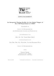
ons to a variable fraction ofpredominantly lose energy in matter by bremsstrahlung, andscatterers [33], and achievehigh-energy photons by e + e − pair production. The characteristicamount of matter traversed for these related interactions is calledthe radiation length X 0 , usually measured in g cm −2 . It is both(a) the mean distance over which a high-energy electron loses allbut 1/e of its energy by bremsstrahlung, 2.4. and Carrier (b) Generation 7 9of the mean and Recombinationfree path for pair production by a high-energy photon [35]. Itis also the appropriate scale length for describing high-energy2.4.2. Generation electromagnetic by Electromagnetic cascades. X 0 has Excitation been calculated and tabulatedby Y.S. Tsai [36]:Ψ 1plane y plane Electrons can be excited =4αr from the 2 N{}valence Ae Z 2 [Linto rad the − f(Z)] conduction + ZL band ′ rad by . absorbing (27.20) a photon with anXenergy larger than the band 0 Agap. This effect is used in photo detectors and solar cells.θ For A = 1 g mol −1 ,4αr planee 2N A/A = (716.408 g cm −2 ) −1 . L rad andIf the energy L supplied ′ radare by given the in photon Tableis27.2. largerThe thanfunction the bandf(Z) gap, the is an electron infinite and the hole willgradually move sum, towards but the forband elements gap edges up to by uranium emitting the canexcess be represented energy into the to crystal lattice asescribe multiple Coulombphonons. The4-place absorption accuracy of energies by smaller than the band gap is possible if intermediate states insidethe band gap are created by impurities f(Z) =a 2 or [(1 imperfections + a 2 ) −1 +0.20206 of the crystalin the plane of the figure.lattice.rojected (plane) angular−0.0369 a 2 +0.0083 a 4 − 0.002 a 6 ] , (27.21)y by [31]⎫2.4.3. Generation where a by = αZ Charged [37]. Particles⎪⎭ dΩ , (27.13)ce20e⎫Charged particles traversing a material lose part of their kinetic energy by electromagnetic interactionswith the electrons and nuclei of the material. rad and LTable 27.2: Tsai’s LThis ′ rad, for use in calculating⎪⎭ dθ plane , (27.14)effect is different for electrons and positronsthe radiation length in an element using Eq. (27.20).compared to heavier particles.n this approximation,Element Z L rad L ′ radx and y axes are orthogonalH 1 5.31 6.144Ω ≈ dθ plane,x dθ plane,y Electrons . and positronsHe 2 4.79 5.621y are independent andLi 3 4.74 5.805quantities sometimes Highusedenergy electrons and Be positrons 4 predominantly 4.71 lose their kinetic 5.924 energy by bremsstrahlungring. They are while at low energiesOthers main > loss 4 isln(184.15 due to ionisation, Z −1/3 ) although ln(1194 Zother −2/3 ) effects like Møller andBhabha scattering contribute as well. The individual contributions for different incident energies= √ 1 θ 0 , (27.15)3 can be seen in figure 2.7= √ 1 x θ 0 , (27.16)3= 10.204 √ 3 x θ Positrons0 . (27.17)Lead (Z = 82)Electrons1.0his section apply only in the0.15nce of large-angle scatters.Bremsstrahlungθ in a given plane aresee Sec. 31.1 of this Reviewcoefficient). Obviously,Ionization0.10the correlation coefficient0.5 Møller (e − )rlo generation of a jointher calculations, it may beBhabha (e + )0.05endent Gaussian randomvariance one, and then setPositronannihilation−1 dE (X −1E dx 0 )3+z 2 ρ yθ x θ 0 / √ 30110 100 1000E (MeV)0/2 ; (27.18)Figure 27.10: Fractional energy loss per radiation lengthFigure (27.19) 2.7.: Fractional in lead energyas loss a function per radiation oflength electron in leador aspositron a function of energy. electronElectronor positron energy [9]. Electron(positron) scattering is considered as ionization when the energy loss per collision is below 0.255 MeV, andane equals x θ plane /2 and (positron) scattering is considered as ionization whenas Møller (Bhabha) scattering when it is above.uld have occurred had theingle point x/2.oulomb scattering hasth various theoreticalthe energy loss per collision is below 0.255 MeV, and asMøller (Bhabha) scattering when it is above. Adapted fromFig. 3.2 from Messel and Crawford, Electron-Photon ShowerDistribution Function Tables for Lead, Copper, and AirAbsorbers, Pergamon Press, 1970. Messel and Crawford useX 0 (Pb) = 5.82 g/cm 2 , but we have modified the figures toreflect the value given in the Table of Atomic and NuclearProperties of Materials (X 0 (Pb) = 6.37 g/cm 2 ).(cm 2 g −1 )27

2. Basics on Silicon Semiconductor TechnologyThe overall energy loss of high energy electrons and positrons can be characterised by the radiationlength X 0 , which describes the average amount of matter that is traversed by the particleswhile loosing 1/e of its kinetic energy by bremsstrahlung. According to [9] a compact fit to datayields:X 0 =716.4·AZ(Z + 1)ln(287 √Z)g cm −2 (2.26)where the atomic number Z > 4 and A is the mass number. For silicon with a density of ρ =2.33 g/cm 3 the radiation length according to equation 2.26 is X 0 = 9.36 g/cm −2 .Other charged particlesThe mean rate of energy loss (or stopping power) of particles other than electrons and positrons isdescribed by the famous Bethe-Bloch equation [9]:where the symbols represent− dEdx = Z [1 1 Kz2 A β 2 2 ln 2m ec 2 β 2 γ 2 T maxI 2− β 2 − δ(βγ) ]2(2.27)Symbol Definition Units or ValueZ atomic number of absorberA atomic mass of absorberK 4πN A rem 2 e c 2 /A 0.307075 MeV cm −1ze charge of incident particlem e c 2 electron mass ×c 2 0.511 keVvβcγ (1 − β 2 ) − 1/2T kinetic energy MeVI mean excitation energy eVδ(βγ) density effect correctionand T max is the maximum kinetic energy which can be imparted to a free electron in a single collision.Figure 2.8 shows the stopping power for positive muons in copper for a wide range of energies.The minimum ionization loss of a muon is located at approximately 350 MeV. For other particlesthe minimum ionisation energy is different, e.g. for pions it is around 470 MeV and for protonsat around 3.2 GeV. Such particles with an energy located at the minimum are called MinimumIonising Particle (MIP). In high energy physics, most particles have mean energy loss rates closeto the minimum and can be considers as MIPs.For a particle detector, MIPs are an important benchmark, as they deposit only a minimum amountof their kinetic energy in the active sensor material. To assess if a sensor is still able to reliablydetect a MIP, the ratio of the induced signal to the noise of the sensor is an important performanceparameter. Therefore, the Signal-to-Noise Ratio (SNR), defined as the ratio of the signal created by28

27.4.5. Bremsstrahlung and pairproduction at very high energies . . . . . . . . 27527.5. Electromagnetic cascades . . . . . . . . . . . 27627.6. Muon energy loss at high energy . . . . . . . . 27727.7. Cherenkov and transition radiation . . . . . . . 278E µc Critical energy for muons GeVE s Scale energy √ 4π/α m e c 2 21.2052 MeVR M Molière radius g cm −2(a) For ρ in g cm −3 .2.4. Carrier Generation and RecombinationStopping power [MeV cm 2 /g]100101Lindhard-ScharffNuclearlossesµ −Anderson-ZieglerBethe-Blochµ + on CuRadiativeeffectsreach 1%[GeV/c]Muon momentumRadiativeRadiativelossesWithout δ0.001 0.01 0.1 1 10 100 1000 10 4 10 5 10 6βγ0.1 110 100 1 10 100 110 100[MeV/c]MinimumionizationE µc[TeV/c]Fig. 27.1: Stopping power (= 〈−dE/dx〉) for positive muons in copper as a function of βγ = p/Mc over nine ordersof magnitude Figurein2.8.: momentum Stopping power (12 orders (〈−dE/dx〉) of magnitude for positive inmuons kineticinenergy). copper asSolid a function curves of indicate βγ = p/mcthe over total ninestopping orders of power.Data below the break magnitude at βγ ≈in0.1 momentum are taken (12from orders ICRU of magnitude 49 [2], in and kinetic dataenergy) higher [9]. energies Solid curves are indicate from Ref. the 1. total Verticalbands indicate boundaries stoppingbetween power. Vertical different bands approximations indicate boundaries discussed between indifferent the text. approximations.The short dotted lines labeled “µ − ”illustrate the “Barkas effect,” the dependence of stopping power on projectile charge at very low energies [3].a single particle to the intrinsic noise of the sensor, caused by MIP-like particles is the most relevantdescription of the sensitivity of a sensor.Equation 2.27 describes only the mean energy loss of a particle in matter, while the actual energyloss of each particle is fluctuating. The statistics of the measurable signal caused by charged particlesis described by the Landau distribution as further discussed in chapter 3.1.2.4.4. Charge Carrier LifetimeThe lifetime of charge carriers in a semiconductor can be described by two parameters, the generationand the the recombination lifetime. They describe the transient behaviour from a state of nonequilibrium,created either due to removal of charge carriers (creation lifetime) or due to injection ofadditional charge carrier (recombination lifetime), back to equilibrium.An excess of minority charge carriers can be created by exposing a semiconductor to a light pulseor to ionising radiation. After this initial event creating the additional charge carriers, it will takesome time to settle back into equilibrium, where the excess minority charge carriers will recombinewith the majority carriers. We assume the overall recombination rate R to be proportional to theproduct of electron and hole concentration:R = βnp = βn 2 i (2.28)A charged particle or a light pulse would cause an additional generation rate G rad . As electrons andholes are created in pairs, it would increase the thermal equilibrium concentration of the minority29

2. Basics on Silicon Semiconductor Technology(n 0 ) and majority (p 0 ) charge carriers by the same amount ∆n = ∆p = ∆. The recombination ratewill increase:R = β(n 0 + ∆)(p 0 + ∆). (2.29)For a direct semiconductor at thermal equilibrium, the average concentration of holes and electronsis constant in time. Nevertheless the thermal creation (G th ) and recombination (R th ) of charge carriersis occurring continuously but the rates for both processes are equal:G th = R th = βn 0 p 0 . (2.30)We can now define an excess recombination rate U which is zero at thermal equilibrium:U = R − R th = β(np − n 0 p 0 ). (2.31)The additional generation rate created by ionising radiation G rad must be compensated by excessrecombination rate U, thus giving:G rad = U = R − R th = β(n 0 + ∆)(p 0 + ∆) − βn 0 p 0 (2.32)= β(n 0 p 0 + n 0 ∆ + p 0 ∆ + ∆ 2 − n 0 p 0 ) (2.33)= β∆(n 0 + p 0 + ∆) (2.34)For low injection levels, were the number of additional charge carriers is small compared to thenumber of majority carriers (∆n ≪ p 0 for p-type and ∆p ≪ n 0 for n-type material), equation 2.34simplifies to:G rad = β p 0 ∆n = ∆nτ rfor p-type material with τ r = 1β p 0(2.35)G rad = βn 0 ∆p = ∆pτ rfor n-type material with τ r = 1βn 0(2.36)The recombination lifetime τ r is a time constant defining the duration until the minority carrierdensity will return to thermal equilibrium.We will now consider the opposite situation, where all charge carriers are removed from the semiconductor,for example by applying an external voltage. In this case, the initial recombinationrate is zero and the generation rate will be equal to the thermal generation rate. With similarconsiderations as before, the time constant for the return to equilibrium is the generation lifetimeτ g :τ g = n i= 1 , (2.37)G th βn iwhich is different from the recombination lifetime.For indirect semiconductors, such as silicon, the relationship between the two lifetimes is more complicated.This is due to the different crystal momentum for holes at the maximum of the valenceband and electrons at the minimum of the conduction band, as already explained in the previoussection. To enable the transfer of momentum to the crystal lattice, recombination in indirect semiconductorshappens in a two step process, involving additional energy states in the forbidden bandgap. These states are created by impurities and defects in the crystal lattice, which can capture andsubsequently release an electron or hole depending on their type.30

2.5. Basic Semiconductor StructuresThe process of capturing a hole or electron is called trapping and the defects in the silicon crystalenabling such processes are referred to as trapping centers. They cause a reduction of thesignal induced by ionising radiation in a silicon sensor, as the trapped charges are captured andonly emitted later. The readout electronics measures the signal carried by the non trapped carrierswhile the trapped charges are released too late. Radiation damage can increase the numberof trapping centers and thus reduce the SNR of the sensor. See section 2.6 for more information.2.5. Basic Semiconductor StructuresUsing the n-type and p-type semiconductor materials described in the previous sections and addingmaterials like insulators and metals, we can create the main building blocks needed to form a siliconsensor. We will describe these basic structures in this section and discuss their most importantproperties.2.5.1. The p-n Junction or DiodeThe simplest semiconductor device is the diode. It can be described as an electronic check valve,enabling the flow of an electric current only in one direction. An equal description would be, that adiode has a low resistance if operated in conducting direction, while being high resistive if operatedin reverse direction.A p-n junction is created by joining a p-type and an n-type material. Beginning at the initial contactof two materials, the electrons from the n-type region will diffuse into the p-type region andrecombine with the holes. This will create a space charge region near the junction, as the electronsdiffusing from the n-type region will leave the donor ions uncompensated. Similarly the holes inthe p-type region are compensated by the electrons and leave the acceptor ions uncompensated. Thebuild-up of charge will counteract the diffusion until a certain depth of the space charge region iscreated, which is depleted of free charge carriers. The situation in the vicinity of the p-n junction isshown in figure 2.9.The band structure in the p-type and n-type material is different prior to putting them into contact.Due to doping, the fermi level E f ermi will move towards the valence band for p-type material andtowards the conduction band for n-type material. Upon contact of the two materials at thermal equilibrium,the fermi level at the p-n junction has to line up. This will shift the valence and conductionband and lead to a so called built-in voltage V bi or diffusion voltage, as seen in figure 2.9 b. We cancalculate V bi using equations 2.12 and 2.13 and setting the majority carrier concentrations equal to31

2. Basics on Silicon Semiconductor Technologyd pd np-type N AN Dn-typea)Energy bandsb)c)d)E CE VE fermiDoping concentrationN AN DCharge densityElectric field-qN AqN DV bie)Electric potentialf)Figure 2.9.: Various parameters in the vicinity of a p-n junction. In diagram a) the donor and acceptor distribution of apartially depleted p-n junction is depicted. Diagram b) shows the energy band structure and c) the concentrationof doping atoms. In diagram d) the charge density is shown, while e) and f) show the corresponding32electric field and potential.

2.5. Basic Semiconductor Structuresthe acceptor and donor concentrations:n n = N D , p p = N A (2.38)N D ·N A = n 2 i exp E pi − Ein (2.39)kTV bi = 1 q (E pi − Ei n ) = kT q ln N AN D. (2.40)n 2 iThe size of the depleted zones in the p-type (d p ) and n-type (d n ) material can be calculated accordingto [7] as:√2εε 0d n =d p =d = d n + d p =q e√2εε 0q eN AN D (N A + N D ) V bi (2.41)N DN A (N A + N D ) V bi (2.42)√2εε 0 (N A + N D )q e N A N DV bi (2.43)For practical applications, p-n junctions are usually formed using a low doped material where acertain region gets highly doped towards the opposite type. The p-n junction is formed at the edgeof the highly doped region which is in contact to the surrounding bulk with low doping concentrationof opposite dopands. In this realistic case where the doping concentration on one side ofthe junction is significantly higher than on the opposite side (e.g. N A ≫ N D ), equation 2.43 becomes:√2εε 0d = V bi (2.44)q e N DIf an external voltage is applied across the p-n junction, the charge carriers will start to drift accordingto the electric field. Depending on the polarity of the applied voltage, the width of the spacecharge region will shrink (forward bias) or expand (reverse bias) and we have to replace the built-involtage V bi with V bi −V :√2εε 0 (N A + N D )d =(V bi −V ). (2.45)q e N A N DFor the realistic case as discussed above with N A ≫ N D , equation 2.45 simplifies to:√2εε 0d = (V bi −V ). (2.46)q e N DCurrent - Voltage CharacteristicsIn equilibrium, the diffusion of electrons (holes) due to the unequal majority charge carrier concentrationsin the p-type and n-type materials is counterbalanced by the drift of electrons (holes)33

2. Basics on Silicon Semiconductor Technologyin the opposite direction induced by the space charge. An external voltage applied to the p-n junctionwill disturb this balance and influence the drift and diffusion currents of the charge carriers.In forward bias direction, the lower electric field in the depleted region will reduce the drift ofelectrons (holes) from the p-side (n-side) to the n-side (p-side). In turn, the diffusion of electrons(holes) from n-side (p-side) to the p-side (n-side) is enhanced as minority carriers are injected intothe junction. Under reverse bias, the electric field is increased and the diffusion of charge carriersis reduced resulting in a very small reverse bias current.The total current density through the junction of an ideal diode can be described by the Shockleyequation:(J = J 0 exp q )eVk B T − 1 (2.47)where the current in reverse bias direction (V ≪ 0) is saturated at saturation current density −J 0while it rises exponentially with the applied voltage in forward bias direction, as seen in figure 2.10.The saturation current density is given by [8]:J 0 = q eD p p n0L p+ q eD n n p0L n(2.48)where D p and D n are the diffusion constants for electrons and holes (see equations 2.25 and 2.24),p n0 and n p0 are the electron densities in the n-side and the hole densities in the p-side at thermalequilibrium and L p = √ D p τ p and L n = √ D n τ n are the diffusion lengths of holes and electrons.J/J 064Forward BiasRegion2-4 -3 -2 -1 1qV/k BTReverse Bias RegionJ 0Figure 2.10.: Ideal current - voltage characteristics of a p-n junction.34

2.5. Basic Semiconductor StructuresCapacitance - Voltage CharacteristicsWe will now derive the capacitance - voltage characteristics for a one dimensional doping profile.As already discussed for equation 2.44, we will consider a simplified but realistic case for sensors,where a very small region of highly dope p-type material is embedded in a n-type substrate. In suchan extremely asymmetric case, the space charge region is fully contained in the low doped n-typesubstrate.To find the capacitance of the space-charge region we need the derivative of the charge Q SCR withrespect to the applied reverse bias voltage V :C = dQ SCRdV= dQ SCR/dWdV/dW(2.49)Increasing the space-charge region by dx will increase the surface charge by q e N D dx, the electricfield by q eN D dxε 0 εand the surface voltage by q eN D dxε 0 εx. Integrating over the full space-charge regiongoing from 0 to W we get the charge and voltage in the region:∫ WQ SCR = −V SCR =0∫ W0q e N D (x)dx (2.50)q e N D (x)x dx (2.51)ε 0 εWe can now calculate the derivatives of the charge and the voltage across the the space-chargeregion with respect to the size of the region. The voltage drop across the space-charge region isdefined by the external voltage, reduced by the built-in voltage V bi defined in equation 2.40. Wenow get:dQ SCRdW = −q eN D (W) (2.52)dVdW = dV bidW − dV SCRdW= k BT 1 dN D (W)q N D (W) dW− q eN D (W)(2.53)ε 0 εFor the inverse capacitance of the junction we get:1C = W ε 0 ε − k BTq1q e N 2 DdN DdW ≈ W ε 0 ε . (2.54)As the variation of the built-in voltage with doping is negligible in comparison to the appliedreverse bias voltage which is usually much higher, we can the corresponding term in equation2.54.The thickness of the space-charge region can now be derived from a capacitance measurement ofthe device as:d = W = ε 0εC . (2.55)35

2. Basics on Silicon Semiconductor TechnologyEquation 2.55 is for a one dimensional p-n junction, while for a real diode with a junction area Athe depletion depth becomes:d = W = A ε 0εC , (2.56)which resembles the situation of a parallel plate capacitor with electrodes of size A at a distance dand a dielectric in between with a dielectric constant of ε.The doping concentration can be derived from the derivative of the inverse square of capacitancewith the applied reverse bias voltage. Using equations 2.55 and 2.51 and again ignoring V bi weget:d(1/C 2 )dVand the doping concentration at depth W is:= d( 1/C 2 )/dWdV/dW = 2W /(ε 0 ε) 2q e N D W/(ε 0 ε) = 2q e N D ε 0 ε , (2.57)N D =2q e ε 0 ε d( 1/C 2 )dV(2.58)Full Depletion VoltageThe voltage at which the depleted space-charge region covers the full depth of the device is calledFull Depletion Voltage V FD . Following equation 2.58 the capacitance of the device will increasewith the reverse bias voltage V until V = V FD . For V ≥ V FD it will remain constant as seen in figure2.111.41.21/C 2 [(C FD) 2 ]10.80.60.40.200 20 40 V FD60 80 100Voltage [V]Figure 2.11.: Plot of a C-V curve of an ideal diode. Before full depletion, the inverse square capacitance rises linearly.At V = V FD the device is fully depleted and the capacitance remains constant.36

2.5. Basic Semiconductor StructuresFollowing equation 2.46 the thickness d of a device can be calculated from V FD for V ≫V bi :√2ε 0 εd = V FD (2.59)q e N DFor practical reasons the doping concentration N D is substituted with the resistivity of the bulkmaterial from equation 2.15 which yields:d = √ 2ε 0 εµ n ρV FD (2.60)In comparison to an ideal diode, the p-n junctions in strip sensors are segmented, which makes theelectric field inside the bulk non-linear due to edge effects. The solutions to the Poisson equationdescribing the voltage drop are more complicated and are discussed in detail in [10]. The solutionfor strip sensors is given by:[V FD,sensor = V FD,diode 1 + 2 p ( )] wd f , (2.61)pwhere p is the pitch between neighbouring strips and w is the width of the strip. The function f (w/p)is a numerical approximation for the solution and is according to [10]:f (x) = −0.00111x −2 + 0.0586x −1 + 0.240 − 0.651x + 0.355x 2 (2.62)For a sensor with a standard width-to-pitch ration of 0.25, the correlations between resistivity, thicknessand full depletion voltage are:√2ε 0 εµ n ρV FD,sensord =1 + 2 p d 0.3161 (2.63)ρV FD,sensord2ρV FD,diode =1 + 2 p =d0.3161 2ε 0 εµ n(2.64)ρV FD,sensor = d2 (1 + 0.6322 p d ) = d2 + 0.6322pd2ε 0 εµ n 2ε 0 εµ n(2.65)2.5.2. The n+-n or p+-p JunctionIn the previous chapter on p-n junctions, the build-up of a space-charge region was explaineddue to electrons diffusing from the n into the p region while holes are diffusing from p to n.The diffusion of electrons and holes stops, when the electric field inside the space-charge regionis high enough. The electrical potential of the space-charge region is called built-in voltageV bi .A similar situation is created in single-type semiconductors if the doping concentration changessignificantly over a small area 1 . In the case for n+-n junctions, electrons from the heavily doped n+region diffuse into the much less doped n region and create a space charge region. The resultingelectrical field counteracts the diffusion and the Fermi levels of the two regions in the band modelare lined up. This again results in a built-in voltage V bi .1 Heavily doped regions are denoted as n+ or p+, hence the name n+-n or p+-p for single-type junctions.37

2. Basics on Silicon Semiconductor Technology2.5.3. The Metal - Semiconductor ContactHistorically, the metal-semiconductor contact was one of the first semiconductor devices showingrectifying properties. As the name suggests, such contacts form at the junction between a metaland a semiconductor of low doping concentration. Such contacts are also called Schottky barriers.The situation at the metal - semiconductor junction is similar to a p-n junction. The Fermi levelE f ermi in the metal and the semiconductor are at different energies. Upon contact, these the levelshave to line up and therefore alter the band structure creating barriers for the charge carriers.Let’s consider the situation of separated metal and n-type semiconductor. The energy necessary tomove an electron from the Fermi level into the vacuum is described by the work function q e Φ m . Thespecific value of Φ m depends on the type of metal and is different to the value Φ s < Φ m in the semiconductorwhich in turn depends on its type and doping. Furthermore we define the electron affinityq e χ which is the difference between the conduction bands edge to the vacuum level in the semiconductor.This value does not depend on the doping of the material.Now we consider the metal and the semiconductor in direct contact, where the Fermi levels in bothmaterials have to line up and a built-in voltage V bi = Φ m −Φ s is created, as the bands will be bent inthe vicinity of the contact. Charge carriers in the semiconductor will move to fulfill the thermal equilibriumcondition at any point, while the situation in the metal is somewhat different. The numberof free electrons in the metal is so huge, that the electric field inside the metal is approximately zero.Therefore the positive space charge region created in the semiconductor will be compensated by asurface charge at the metal side. This creates a barrier for electrons diffusing from the metal to thesemiconductor side. The height of the barrier can be described by:q e Φ Bn = q e (Φ m − χ) (2.66)This barrier is not influenced by an external bias voltage, while the threshold for electrons travelingin the opposite direction will change. This rectifying function is similar to a diode with a lowforward voltage drop. For strip sensors, Schottky barriers are created at the interface of the semiconductormaterial to the metallisation for external connections. Their rectifying properties are anuisance and should be avoided by using highly doped silicon at the interface. The high doping concentrationwill decrease the width of the potential barrier and tunneling of electrons becomes moreimportant as described in [8]. The characteristic resistance in the metal to semiconductor directionwill be negligible and the contact will show an ohmic behaviour.2.5.4. The Metal - Oxide - Semiconductor StructureThe Metal - Oxide - Semiconductor (MOS) structure is a very important component widely usedin the semiconductor industry. One example utilizing MOS structures are Charge Coupled Devices(CCD) which are used as imaging sensors. For silicon strip sensors, MOS structures are usuallyonly used as test structures to provide access to the measurement of interface properties.38

2.5. Basic Semiconductor StructuresA MOS structure consists of a semiconductor covered by an insulator which is often made of silicondioxide (SiO 2 ) but can be composed of any material with insulating properties. To understandthe functionality of the structure, we have to understand the distribution of charge carriers insidethe semiconductor device and at the interface between semiconductor and insulator for differentexternal voltages applied between the metal contact and the semiconductor. We will first considera simplified situation for a n-type semiconductor in thermal equilibrium, neglecting any chargecarriers in the oxide. Depending on the externally applied voltage we can distinguish four differentsituations: flat band, accumulation, depletion and inversion.Flat Band Situation (V = V FB )Let us consider a more simplified situation first, where the work functions (the energy necessary tomove an electron from the Fermi to the vacuum level) for metal and semiconductor are equal. Withoutthe application of an external voltage, the electrons in the n-type semiconductor are uniformlydistributed and the electric field will be zero everywhere along the device. No external voltage isneeded to achieve this situation and the flat-band voltage V FB is zero.In a more realistic situation, the work functions for an electron in the metal and in the semiconductorare different, while the vacuum level is constant throughout the device, as we considered the oxideto be free of charges and therefore without an electric field. To achieve this situation we have toapply an external voltage V FB between the metal electrode and the semiconductor to compensatethe different work functions:V FB = Φ m − Φ s (2.67)The situation is represented in figure 2.12.Accumulation Situation (V > V FB )If the externally applied voltage exceeds the flat band voltage, the bands at the oxide - semiconductorinterface will bend down. Electrons will accumulate in a thin layer at the surface as the Fermilevel moves closer to the conduction band edge. The thermal equilibrium condition must be fulfilledwithin the semiconductor:n= exp E f ermi − E i(2.68)n i k B Twhere n is the actual and n i the intrinsic charge carrier concentration. The surface charge density isgiven by:Q acc = −ε 0 ε oxV −V FBd ox= −C ox (V −V FB ) (2.69)where C ox is the capacitance per unit area of the oxide layer.The situation is represented in figure 2.13.39

2. Basics on Silicon Semiconductor TechnologyMetalOxideSemiconductora)Energy bandsb)E fermiq Φq e Χe m q e Φ s-q e V FB q ΨVacuum LeveleBE CE fermiE fermi,iE VCharge densityc)Electric fieldd)Electric potentiale)Figure 2.12.: An n-type MOS structure in the flat band situation V = V FB . The oxide is considered to be free of charges.40

2.5. Basic Semiconductor StructuresMetalOxideSemiconductora)Energy bandsb)-q VeE fermiq ΦElectronsq Χ eq e Φ se mq e Ψ BVacuum LevelE CE fermiE fermi,iE VCharge densityd)Electric fielde)Electric potentialf)Figure 2.13.: An n-type MOS structure in the accumulation situation V > V FB . The oxide is considered to be free ofcharges.41

2. Basics on Silicon Semiconductor TechnologyDepletion Situation (V < V FB )If the externally applied voltage is smaller than the flat band voltage V FB , the bands at the oxidesemiconductorinterface will bend upwards. The concentration of electrons near the interface willdecrease and a depleted region will build up.According to [7], the depth of the depletion layer is given by:√( )ε 0 ε 2sεsd s = (V FB −V ) + d ox − ε sd ox (2.70)q e N D ε ox ε oxThe situation is represented in figure 2.14.Inversion Situation (V ≪ V FB )If the external voltage is much smaller than the flat band voltage V FB , such that the intrinsic levelat the oxide-semiconductor interface q e Φ B is higher than the Fermi level q e Φ s , a majority of holeswill accumulate at the interface. For Φ s = −2Φ B the hole density at the interface equals the electrondensity in the bulk of the semiconductor. This situation as also called strong inversion. Thedepletion depth reaches its maximum and even a further increase of the external voltage will notchange the depth:√4ε 0 ε s Φ Bd max = . (2.71)q e N DThe situation is represented in figure 2.15.Oxide ChargesIn a real MOS structure, composed of silicon and silicon dioxide, charges will be present insidethe oxide and at the Si-SiO 2 interface which will change the flat band voltage V FB . The changedepends on the amount and distribution of the charges ρ(x) inside the oxide and can be describedas:∆V FB,oxB = 1 ∫ doxρ(x)x dx. (2.72)ε 0 ε oxThe change due the interface region can be described as a thin layer of charges with a density of σat a distance d ox from the metal:∆V FB,oxI = − σd oxε 0 ε ox. (2.73)Equation 2.67 has to be corrected for these to effects and becomes:V FB = Φ m − Φ s − 1 [ ∫ dox]σd ox + ρ(x)x dx . (2.74)ε 0 ε ox 0042

2.5. Basic Semiconductor StructuresMetalOxideSemiconductora)Energy bandsVacuum Levelq e Φ mq Ψb)Efermi q e Χ q e Φ s-q e VE CE fermiq e Ψ seBE fermi,iE VCharge densityd)Electric fielde)Electric potentialf)Figure 2.14.: An n-type MOS structure in the depletion situation V < V FB . The oxide is considered to be free of charges.43

2. Basics on Silicon Semiconductor TechnologyMetalOxideSemiconductora)Energy bandsb) E fermi-q V eCharge densityq e Φ mVacuum Levelq eΧ q e Φ sq Ψq Ψ e sHoleseBE CE fermiE fermi,iE Vd)Electric fielde)Electric potentialf)Figure 2.15.: An n-type MOS structure in the (weak) inversion situation V ≪ V FB . The oxide is considered to be free ofcharges.44

2.6. Radiation Damage and the NIEL hypothesisCapacitance - Voltage CharacteristicsThe capacitance of the MOS structure is measured by applying a small AC-voltage on top of theDC bias voltage. The response from the structure depends on the relationship between the frequencyof AC-voltage and the time it takes for the structure to return to equilibrium. The measuredcapacitances are strongly frequency dependent.For low frequencies we can assume (C ox = ε 0ε oxd ox, C s = ε 0ε sd s):Accumulation region C = C oxDepletion region C = C oxC sseriesC ox +C sas the capacitance of the oxide and the depletion layer appear inInversion region C = C ox as the depletion layer stays constant, while the surface charge densityvaries with the applied voltage.At high frequencies the measured capacitance again appears as C= C oxC sC ox +C s, because the depletionlayer depth varies with the voltage while the surface charge density stays constant.2.5.5. The Polysilicon ResistorResistors of a wide range of resistances can be created by depositing and doping a layer of polysilicon.Pure polysilicon has a resistivity of 230 kΩcm which can be adjusted to the appropriate valueby doping. Special attention has to be made when contacting polysilicon resistors with metal due tothe Schottky barrier described in section 2.5.3. Usually a good electrical contact between metal andthe resistor is achieved using a heavily doped area of polysilicon to make the contact to the metal.This structure is also called a Polysilicon Head.2.6. Radiation Damage and the NIEL hypothesisThe effects of radiation on silicon sensor have to be carefully evaluated to ensure proper operationover the full length of an experiment’s expected lifetime. Even today, most effects are only partlyunderstood. We have to rely on careful evaluation of radiation experiments and parametrization ofthe resulting effects, without a complete understanding about the physical background.The silicon sensor have to endure a variety of radiation types, which, for simplicity, we are goingto divide into two types:• Charged particles like protons, pions, electrons, . . .• Neutral Particles like neutrons45

2. Basics on Silicon Semiconductor TechnologyNeutral particles interact by elastic or inelastic scattering with the semiconductor nucleus, whilecharged particles like protons or electrons scatter by electrostatic interaction as well. The mass ofthe scattering particle is also important, because it limits the maximum energy that can be transferredfrom the incident particle to a lattice atom. Electrons, for example, seldom create latticedefects as they cannot transfer enough energy and cause point defects and ionization only. In table2.2 some important characteristics of the primary interactions of radiation are given. The conceptsof point and cluster defects will be clarified later.Radiation Electrons Protons Neutrons Si +Interaction Coulomb Coulomb Elastic Coulombscattering and nuclear nuclear scatteringscattering scatteringT max [eV ] 155 133,700 133,900 1,000,000T av [eV ] 46 210 50,000 265E min [eV ]point defect 260,00 190 190 25defect cluster 4,600,000 15,000 15,000 2,000Table 2.2.: Characteristics of interaction of radiation with silicon [7]. The radiation energy is 1 MeV, T max is the maximumkinematically possible recoil energy, T av the mean recoil energy and E min the minimum radiation energyneeded for the creation of a point defect and for a defect cluster.Figure 2.16 shows the Non Ionizing Energy Loss (NIEL) for different particle energies. The damagecaused by different types of radiation can be compared using the hardness factor κ which isdefined according to [11]:Φ 1MeVeq = κΦ (2.75)where κ is defined as:κ =EDKEDK(1MeV )with EDK the Energy spectrum averaged Displacement KERMA 2EDK =(2.76)∫ D(E)Φ(E)dE∫ Φ(E)dE(2.77)where Φ(E) is the differential flux and∫D(E) = ∑σ k (E)kdE R f k (E,E R )P(E R ) (2.78)is the displacement KERMA or the damage function for the energy E of the incident particle, σ kthe cross section for reaction k, f k (E,E R ) the probability of the incident particle to produce a recoilof energy E R in reaction k and P(E R ) the partition function (the part of the recoil energy depositedin displacements). The normalised EDK for 1 MeV neutrons is EDK(1 MeV)=95 MeVmb. Theintegration is done over the full energy range.2 Kinetic Energie Released per unit MAss (KERMA) is the sum of the initial kinetic energies of all the charged particlesliberated by uncharged ionizing radiation (neutrons and photons) in a sample of matter, divided by the mass of thesample. It is measured in Gray.46

2.6. Radiation Damage and the NIEL hypothesisThe hardness factor κ now becomes:κ 1 MeV n =∫ D(E)Φ(E)dE95 MeV mb·Φ(2.79)Using the hardness factor κ 1 MeV n , the NIEL hypothesis allows the scaling of the damage causedby any charged particle to 1 MeV neutrons.2.6.1. Bulk and Surface DamageIn this section we are going to investigate the effects of the two types of radiation (neutral andcharged particles) on the semiconductor lattice and the insulating oxide layer. As we have learnedfrom the preceding section, the interaction depends on whether the particles are charged or not andon their mass.The actual detection process occurs in the depleted space-charge region of the silicon bulk. Imperfectionsin the crystal lattice would influence the detector properties, generally degrading the sensorperformance. Defects created by radiation which dislocate silicon atoms from their lattice site arethe main concern. As mentioned before, heavy particles scatter with the silicon nucleus and transferkinetic energy to it. If the energy transferred exceeds about 15 eV, a dislocation of a lattice atom ispossible. More specifically, at a recoil energy of about 25 eV, the probability of displacement of asilicon lattice atom is roughly one half.Recoil energies below 1 - 2 keV create only isolated point defects, between 2 keV and 12 keV theenergy is high enough to create one defect cluster and additional point defects and above 12 keVseveral clusters and additional point defects can be produced. A cluster is a dense agglomerationof point defects that appear at the end of a recoil track where the incident particle loses its last 5- 10 keV of kinetic energy and the elastic scattering cross-section increases by several orders ofmagnitude.In the insulating oxide layer which separates the p-type silicon from the aluminium readout strips,the situation is different. The structure is already highly irregular, therefore the interaction of radiationwith the nucleus can be ignored. The additional damage to the oxide structure will not alterthe properties of that region.Much more important is the ionization caused by charged particles, and by photons. One mayconsider the oxide as a region with a high density of defects whose charge state can be altered byirradiation. New electrons and holes are created in the oxide layer. The electron mobility is severalorders of magnitude larger than that of holes. Compared to holes, radiation-generated electrons willdiffuse out of the insulator in relatively short time and the capture of holes is the dominant processthat changes the oxide’s properties. Radiation damage of oxide manifests itself as a buildup ofpositive charge due to semipermanent trapping centers, which causes a shift in the flat-band voltagewhich can be measured.47

2. Basics on Silicon Semiconductor TechnologyFigure 2.16.: Non ionizing energy loss of different particles [12]. The cross sections are normalized to 1 MeV neutronsof equivalent fluence Φ eq .2.6.2. Changes in Properties due to Defect ComplexesThe defects in detector bulk material are still mobile at room temperature. Part of those defects willeven vanish either by an interstitial filling a vacancy or by diffusing out of the surface. However,they may become stable by interacting with another radiation induced defect, or with an imperfectionfrom the crystal growth process. Let’s have a look on the effects and changes in detector propertiesthat are caused by these stable defects. Before going into depth, it is worth mentioning thatthese defects can have one of the following main consequences:• Alterations of charge density in the space - charge region• Formation of recombination - generation centers• Formation of trapping centersAlterations of Charge Density in the Space - Charge RegionThe original dopants such as phosphorus or boron may be captured into new defect complexes,thereby loosing their original function as flat donors or acceptors. They may assume a charge statedifferent from the original one. This will change the effective doping of the semiconductor. Infigure 2.17 the fluence dependence of the effective doping of an originally n-type silicon can beseen. The dashed lines correspond to the parametrisation of that effect. At a certain fluence, thesilicon even changes it’s doping state from n-type to effectively p-type. This effect is called typeinversion.48

2.6. Radiation Damage and the NIEL hypothesisFigure 2.17.: Fluence dependence and parameterisation of the effective doping according to equation 2.80 for an n-typesilicon wafer irradiated with neutrons [13]. The data has been corrected for self-annealing during theextended irradiation period.The effective doping concentration can be parametrised by:N e f f (Φ) = N D,0 e aΦ − N A,0 − bΦ (2.80)with N D,0 and N A,0 being the donator and acceptor concentration before irradiation and a and bconstants to be determined experimentally.A consequence of the alterations in the space charge region is the change of the full depletionvoltage V FD and therefore the operating voltage of the sensor.Recombination - Generation Centers These defects can capture and emit electrons or holesand raise the volume-generated leakage current. The leakage current as a function of the fluenceis shown in figure 2.18. A linear relationship between current and fluence is found. It can beparameterized as:∆I vol= αΦ, (2.81)Vwhere the leakage current damage parameter α is according to [14]:α = (3.99 ± 0.03) × 10 −17 A/cm. (2.82)Trapping Centers Another problem is the trapping of an electron or hole and remission a shorttime afterwards. The charge is released too late to contribute to the signal. The signal mea-49

2. Basics on Silicon Semiconductor TechnologyFigure 2.18.: A 1 MeV neutron equivalent fluence dependence and parameterization of the volume-generated currentfor an n-type silicon wafer irradiated with neutrons [13]. The data has been corrected for self-annealingoccurring during the extended irradiation period.sured by the readout electronics is smaller while exhibiting more noise resulting in a reducedSNR.We present a global parameterization of the fluence dependence of the trapping time:1τ t= 1τ t0+ γΦ (2.83)where τ t is the average time a hole/electron stays trapped and τ t0 is the value before radiation. Thisparameterization works well for hole and electron trapping at moderate fluence. A value of γ ≈0.24 × 10 −6 cm 2 /s is foundFor electrons at high fluences, a steeper increase of trapping probability was observed (see figure2.19).2.6.3. AnnealingObserving a sensor after an extended period of exposure to irradiation, one notices that the damageeffects diminish with time. This effect is called annealing. The rate of damage decrease is stronglydependent on temperature.This effect can naively be interpreted as diffusion of radiation induced crystal defects out of thedetector bulk and, more importantly, by the recombination of vacancies and interstitials. Still, one50

2.6. Radiation Damage and the NIEL hypothesisFigure 2.19.: A 1MeV neutron equivalent fluence dependence and parameterization of the inverse trapping time constantfor holes (open symbols) and electrons (solid symbols) for an n-type silicon wafer irradiated with neutrons[13].must keep in mind that annealing is a rather complicated process involving many different and onlypartially understood interactions between defects and defect complexes.In figure 2.20 the annealing of the radiation induced changes of effective doping is shown over anextended period of time at constant room temperature (20 ◦ C). One may notice an inversion of theannealing effect on the time scale of months.2.6.4. Reverse AnnealingThe inversion of the annealing process is called reverse annealing. Following the initial annealingof irradiated silicon sensors, the effective doping concentration is increasing again after a fewweeks to months at room temperature. This surprising effect can be explained as the transformationof radiation induced electrically inactive defect complexes into electrically active ones. Reverseannealing is also strongly temperature dependent. Below approximately 0 ◦ C the process is almostcompletely suppressed.51

2. Basics on Silicon Semiconductor TechnologyFigure 2.20.: Room temperature annealing of radiation induced changes of effective doping [13]. Data are corrected tocorrespond to a short irradiation followed by a longterm observation at constant (20°C) temperature. Adecrease of the effective doping concentration can be observed on the time scale of weeks (annealing),followed by a rise (reverse annealing) on the time scale of months after irradiation.52

A semiconductor detector is a device that uses a semiconductor (usually siliconor germanium) to detect traversing charged particles or the absorption ofphotons. In the field of particle physics, these detectors are usually known assilicon detectors. When their sensitive structures are based on a single diode,they are called semiconductor diode detectors. When they contain many diodeswith different functions, the more general term semiconductor detector is used.Semiconductor detectors have found broad application during recent decades,in particular for gamma and X-ray spectrometry and as particle detectors.Wikipedia on Semiconductor detector3Silicon Strip SensorsSilicon strip sensors are the favored tracking devices in most modern high energy physics experiments.The basic design has not changed much over the last few centuries since the first stripsensor in planar technology was developed for the NA11 experiment at CERN[15]. Nevertheless,improvements were made to the designs and the production techniques used to manufacture suchdevices. The current status of commonly used design and production principles will be reviewed inthis chapter.3.1. Working PrincipleThe main purpose of a strip sensor is the precise spatial tracking of ionizing particles. The effectused to create a measurable signal from a particle passing the sensor is based on the electromagneticinteraction of the particle with the the silicon bulk. The resulting generation of a currentinside the bulk was described in section 2.4.3 for charged particles and in section 2.4.2 for photons.The amount of charge created by a single particle is very small compared to the intrinsic chargecarrier density. With a mean energy loss of a MIP in silicon of (dE/dx) mean = 388 eV/µm ([16]) anda mean energy for electron-hole creation in silicon of E pair = 3.63 eV (see table 2.1) the number ofelectron-hole pairs created by a MIP in t Sensor = 300 µm silicon becomes:(dE/dx) mean ×t Sensor 388 × 300= ≈ 32 × 10 3 e − h + pairs. (3.1)E pair 3.6353

3. Silicon Strip SensorsThe intrinsic charge carrier generation at T = 300 K for silicon is n i = 1.45 × 10 10 . For siliconwith the same thickness of t Sensor = 300 µm as before and an area of A Sensor = 1 cm 2 this amountsto:n i . t Sensor . A Sensor = 1.45 × 10 10 . 300 . 1 × 10 −4 ≈ 4.4 × 10 8 . (3.2)The signal created by a MIP would be four orders of magnitude lower than the intrinsic noise createdby 1 cm 2 of silicon. Therefore it is necessary to significantly reduce the number of intrinsic chargecarriers. One way would be to operate the sensor at very low temperatures, but a much more practicalway is the usage of a p-n junction operated in reverse bias mode.The main sensor element of modern strip sensor is the depleted zone of a p-n junction. Figure 3.1shows the basic working principle where the p-n junction is operated in reverse bias mode. Forpractical reasons, the junction is very asymmetric while making the depleted region occupy mostor the full depth of the silicon substrate. Therefore the silicon bulk is made of pre-doped material(usually n-type) and the junction is formed by heavy doping of a small surface layer (usually p+type).To make the full depth of the bulk sensitive, it is necessary to fully deplete it by a sufficientlyhigh reverse bias voltage.When an ionising particle particle traverses the depleted region, it creates electron-hole pairs. Due tothe electric field inside the bulk, these charge carriers start to drift towards the electrodes (see section2.3.1) and thereby induce an electric current which can be measured.p-type siliconVn-type siliconFigure 3.1.: Charge generation of an ionizing particle inside the depleted silicon bulk. The charges will drift to theelectrodes due to the electric field and induce a current which can be measured.The energy deposition in thin layers is considerably non-deterministic and the statistical fluctuationsare very asymmetric following a Landau distribution as seen in figure 3.2. It was first described in[17] with a more elaborate discussion and corrections to the distribution in [18].As calculated above, the mean number of electron-hole pairs is about 32.000 but due to the Landaulike behaviour of the energy deposition, the most probable number of electron-hole pairs becomes54

shown clearly in Fig. 1 of Ref. 25 for an argon-filled TPC cell. calculated this waAlso see Talman [26]. While ∆ p /x may be calculated adequately density that matwith Eq. (27.8), the distributions are significantly wider than Refs. 18 and 27,the Landau width w =4ξ [Ref. 24, Fig. 15]. Examples for thin interpolation coeffisilicon detectors are shown in Fig. 27.7.3.1. Working Principle tion for the chempounds. If a comp∆/x (MeV g −1 cm 2 )recipe for δ given0.50 1.00 1.50 2.00 2.50 〈I〉 according to tf (∆/x)1.00.80.60.40.2∆p/xw500 MeV pion in silicon640 µm (149 mg/cm 2 )320 µm (74.7 mg/cm 2 )160 µm (37.4 mg/cm 2 )80 µm (18.7 mg/cm 2 )Mean energyloss rate0.0100 200 300 400 500 600∆/x (eV/µm)Figure 27.7: Straggling functions in silicon for 500 MeVpions, normalized to unity at the most probable value δ p /x.The width w is the full width at half maximum.Figure 3.2.: Straggling functions in silicon for 500 MeV pions, normalised to unity at the most probable value δ p/x [16].The width w is the full width at half maximum.with (dE/dx) MPV = 276 eV/µm:1.000.95(dE/dx) MPV ×t Sensor 276 × 300= ≈ 23 × 10 3 e − h + pairs.E pair 3.63(3.3)0.90The most probable value is the number often used in literature.0.85(∆p/x) / dE/dx minThe electron-hole 0.80pairs created by the incident particle drift towards the electrodes and create anelectric current. The signal is induced by the movement of the charges through electromagnetic interactionand is0.75proportional to the carrier mobilities according to Ramo’s theorem [19]:x = 640 µm (149 mg/cm 2 )320 µm (74.7 mg/cm 2 )0.70J 0 = q e ( )d ∑ ν n +∑ν p , (3.4)0.65where d is the detector thickness, q e the elementary charge and ν n and ν p the drift velocities for0.60electrons and holes.160 µm (37.4 mg/cm 2 )80 µm (18.7 mg/cm 2 )0.55The maximum charge which can be collected by integrating amplifiers, can be calculated by the0.50time integral over the 0.3induced1 current: 3 10 30 100 300 1000∫ tint∫ βγ tint(= p/m)q e ( )QFigure 27.8: 0 = JMost probable 0 dt =energy d ∑ ν n +∑νloss in psilicon, dt,scaled (3.5)27.2.7. Ionizatienergy loss to thetrack. This relatidue to the wandranges exceed thqualitative appravarious media bysee Ref. 28. Thepair produced, Wparticles, increasW can be surpricontaminants [29cases may be grerecombination [3027.3. MultiplAchargedpartsmall-angle scattescattering from nCoulomb scatteristrong interactionCoulomb scatterinof Molière [31].angles, but at largit behaves like RuaGaussiandistribIf we definethen it is sufficieapproximation fodistribution, with13.6 Meθ 0 =βcpHere p, βc, andnumber of the incscattering medium00value of θ 0 is fromto the mean loss of a minimum ionizing particle, 388 eV/µm charged particleswhere t int is the integration(1.66 MeV g −1 time ofcm 2 the amplifier. The measured signal can be reduced due to).better for 10 −3

3. Silicon Strip Sensorsan important parameter and a subject of interest when analysing the radiation hardness of a sensor:CCE = Q cQ 0, (3.6)where Q c is the charge collected in an actual measurement.3.2. Design Basics of a Silicon Strip SensorUsing the basic working principle described in the previous section, it is possible to detect a particlehitting the sensor. It does not give any additional information on the location of the hit on the sensor.This can be achieved by creating smaller sensing elements based on the same principle which areelectrically isolated from each other but located on the same sensor. For practical reasons, we candistinguish two different approaches:Pixel Sensor have very small quadratic or rectangular shaped sensor elements called pixels. Dueto their almost symmetric layout, they provide two dimensional spatial resolution. Each ofthe pixel is readout by a dedicated amplifier which is in some designs also responsible forbiasing it. Pixel sizes are usually very small, in the order of one hundred microns, whichresults in a very high number of pixels per sensor area. Due to the high number of readoutchannels, the costs per area covered by sensors is very high. Due to their inherent radiationhardness, they are used as the innermost tracking layers as in the CMS tracker (see section1.1.1).Strip Sensor have narrow and long asymmetric strips as basic sensor elements. The strips usuallyextend the full length of the sensor, therefore giving only one-dimensional information onthe location of the hit on the sensor. The biasing of the strips is usually fed from a sharedconnection line. The width is in the order of tens of microns, while the pitch between stripscan be from 50 µm up to several hundreds of microns. The much lower density of sensorelements compared to pixel sensors, significantly reduces the number of readout channels.This makes strip sensors comparatively cheaper in terms of costs per sensor area, thereforemaking it the optimal choice for the large areas of the outer tracking layers as in the CMStracker (see section 1.1.2).The following section will review the design basics of standard silicon strip sensors. A 3D-model ofthe full layout as used in the CMS experiment is shown in figure 3.3.3.2.1. Strip GeometryFor practical reasons, only the upper electrode of a strip sensor is segmented into strips, whilethe lower electrode called backplane covers the full backside of sensor. The readout electronicsis connected to each strip and collects the charges generated by incident particles. The strip pitchdepends on the requirements of the spatial resolution and the density of readout channels. Thewidth of the strips, or - more importantly - the ratio between width and pitch (width-to-pitch ratio56

3.2. Design Basics of a Silicon Strip Sensor1.3 Working Principle of a Silicon Tracking Device 25alignmentmarkerpassivationSiO 2 oxidecoupling capacity oxideSiO 2n++ ringbias ringguard ringpassivationDC-padAC-padstrip p+ implantsAl stripsopeningsbiasresistorviasviasn++ ringp+ implantsn++ layern-bulkaluminium backplaneFig. 1.19 A 3D schematic is sketched. It shows the baseline of the CMS sensor at the LHC inFigure 3.3.: 2008, 3D-model but could of a standard representsilicon basically strip any sensor single-sided as usedAC-coupled, in the CMS experiment. R poly biasedIt sensor. features In operation, AC-coupled readoutthe strips bias with ring polysilicon is connected biasing to GND and no potential, intermediate whichstrips is then anddistributed the activetoarea theisp+ protected implantby strips, a single guardwhile ring structure. the Al backplane Illustration is set kindly to positive taken from high [20]. voltage depleting the full n-bulk volume by forminga pn-junction p+ strip to n-bulk. The coupling capacitor is defined between aluminium strip andp+ implant, the inter-strip capacity between neighbouring strips (both p+ and Al part). The guardring shapes the field at the borders. The n++ ring defines the volume and prevents high field in thereal cut edge regionsr wp ) is driven by the balance of low capacitance between the strips (low r wp ) and the need to reducethe field peak at the implant edges.All individual isolated strips need to be at the same potential. This is realized inThe usage one of intermediate of three different strips ways, which illustrated are not in read Fig. 1.20, out, although can increase nowadays the spatial the polysiliconmethod sharing is most between utilized. adjacent 15 strips, while keeping the density of readout channelsresolution bycapacitive chargeconstant. To take advantage of such a strip geometry, the readout has to measure the height ofthe signal which polysilicon is generally biasingreferred to aspunchthrough analogue biasing readout. In comparison, FOXFET biasing a digital readoutpolysilisononly checks, if the signalsmall gapgateresistor exceeds biasa certain threshold while biasdiscarding the actual signal bias height.DC padringDC padringDC padringTherefore such Al strip a technology cannot take Al strip advantage of interpolation Al stripalgorithms based on chargesharing.p+ p+SiO 2n+Al backplanen-bulkSiO p+n+ n-bulkp+2SiO 2Al backplanep+n+ n-bulkp+Al backplaneFig. 1.20 There are three ways to bias an AC-coupled sensor plus a fourth one for a DC-coupleddevice. The punchthrough and FOXFET biasing are the easiest ones but not as radiation hard asthe polysilicon resistor, which is more or less the current standard. A photo of a polysilicon resistorcan be seen in Fig. 1.28. In addition, a DC-coupled device can be biased via the connections to theelectronics, representing the ground potential3.2.2. DC to AC coupled StripsAs described in section 2.5.1 a p-n junction in reverse bias operation still shows a small reversebias current. In an actual sensor, each strip exhibits such a small DC current in the order of nA. Inheavily irradiated 15 Punchthrough strip sensors, and FOXFET the reverse biasing is bias lesscurrent radiationcan hard, rise it significantly be imagined by for several the futureorders ofmagnitudeInternationalreaching aLinearfew µAColliderper strip.(ILC).The amplifiers in the readout chips have to be protected from this current using current compensationcircuits. These high pass filters remove the DC fraction of the current, allowing only the AC signalsto pass to the amplifier. This functionality can also be incorporated into the sensor using largecapacitors between the implant and the readout connection for the chips.57

3. Silicon Strip Sensorsn++ ring strip p+ implantsbias ringguarpassivationDC-padAC-padThe readout capacitors are created by covering the strips with an aluminum electrode of about equalsize above the strip implant, separated by a thin layer of oxide. The capacitance of this parallel-platecapacitor can be maximized by minimizing the thickness of the oxide according to C = ε · A/d. Itoffers good filtering of DC currents, while having a strong coupling of the AC signals to the readoutelectrode which are connected to the amplifiers of the readout chip.Al stripsWhile DC coupled strips can be biased from the readout electronics, a separate biasing scheme isrequired for AC coupled sensors.eningsbiareviasn-bulk3.2.3. Biasing of the StripsFig. 1.19 A 3D schematic is sketched. It shows the baselin2008, but could represent basically any single-sided AC-coupthe bias ring is connected to GND potential, which is thenwhile the Al backplane is set to positive high voltage depletina pn-junction p+ strip to n-bulk. The coupling capacitor is dp+ implant, the inter-strip capacity between neighbouring strring shapes the field at the borders. The n++ ring defines thereal cut edge regionsEach strip needs a reverse bias voltage to deplete the underlying sensor bulk from charge carriers.An aluminium metallisation covering the full backside of the sensor will serve as contact to the bulk.Each of the strip implants themselves needs to be connected to the other polarity of the reverse biasvoltage. In DC coupled sensors this can be provided by the readout electronics which are directlyconnected to the implant.In AC coupled devices 1 the biasing of the strips has to be done by additional structures on thesensor. For practical reasons, they are connected to a ring surrounding the sensor called bias line,which provides the same potential to all of the strips from a single connection to the external voltagesupply.This way all of the strips would be shorted together. To electrically isolate the strips from eachother, each strip is connected to the bias ring using a resistor. Additionally they also serve ascurrent protection for each strip. These resistors can be implemented in various ways (all picturesfrom [20]):All individual isolated strips need to be at the samone of three different ways, illustrated in Fig. 1.20, aPolysilicon resistor A resistor made of doped polysilicon is embedded in the sensor. It has alinear ohmic behaviour and is very radiation hard. The additional deposition and structuringcon method is most utilized. 15of polysilicon requires additional process steps during manufacturing of the sensor, makingthe device more expensive.Al strippolysilicon biasingDC padpolysilisonresistor biasringAl strippunchthrough biasingDC padsmall gapbrSiO 2p+ p+n+ n-bulkSiO 2p+n+n-bulkAl backplaneAl backplane1 Many DC-coupled device implement a form of external biasing from a common bias connection as well to allow theelectric testing of the device. Otherwise each of the strips would need an individual connection to the bias voltage.Furthermore strips which are not properly connected to the readout electronics in the final detector cannot be properlydepleted without a common bias scheme.58Fig. 1.20 There are three ways to bias an AC-coupled sensodevice. The punchthrough and FOXFET biasing are the easithe polysilicon resistor, which is more or less the current standcan be seen in Fig. 1.28. In addition, a DC-coupled device canelectronics, representing the ground potential

plantss. The n++ ring defines the volume and prevents high n-bulk field in thealuminium backplane3.2. Design Basics of a Silicon Strip Sensorrips need to be at the same potential. This is realized inillustrated in Fig. 1.20, although nowadays the polysili-Fig. 1.19 A 3DFOXFETschematicA small gapisbetween sketched.the stripItimplant showsandthe biasbaselinering is coveredof thebyCMSa metal-oxidesensor at the L2008, but could represent structure. Similar basically to a Metal-Oxide any single-sided Semiconductor AC-coupled, Field Effect Transistor R poly (MOSFET) biased the sensor. In opeeffective resistance of the gap can be controlled using a small voltage applied to the metalthe bias ring is connected to GND potential, which is then distributed to the p+ implantgate. This structure is often referred to as FOXFET, as it utilizes the thick Field OXide aswhile the Al backplane gate insulator. is set Cheaper to positive but less radiation high hard voltage than polysilicon depleting resistors. the full n-bulk volume by fa pn-junction p+ strip to n-bulk. The coupling capacitor is defined between aluminium stp+ implant, the inter-strip capacity between FOXFET neighbouring biasing strips (both p+ and Al part). Thering shapes the field at the borders. The n++ ring defines the volume and prevents high field. 15 punchthrough biasingsmall gapbiasreal cut edge DC regions padringAl stripp+ p+Al stripDC padgatebiasringSiO 2 n+ n-bulkSiO p+ p+2 n+ n-bulkAll backplane individual isolated strips need Al backplane to be at the same potential. This is realione of three different ways, illustrated in Fig. 1.20, although nowadays the poo bias an AC-coupled sensor plus a fourth one for a DC-coupledcon OXFET method biasing is are most theutilized. easiest ones 15 but not as radiation hard asless radiation hard than polysilicon resistors.more or less the current standard. A photo of a polysilicon resistorion, a DC-coupled device can be biased via the connections to thepolysilicon biasingpunchthrough biasingnd potentialAl stripPunch through Very similar to a FOXFET but without a gate and a smaller gap. The size of thegap and the electric properties of the oxide define the resistance of the structure. Cheaper butDC padbiasing is less radiation hard, it can be imagined for the futureSiO p+ p+2 n+ n-bulkSiO p+n+ n-bulkp+2C).Al backplanepolysilisonresistorbiasringAl stripDC padAl backplanesmall gapbiasringSiO 2Al stripp+n+FOXFET biasingDC padAl backplanen-bulkFig. 1.20 There are three ways to bias an AC-coupled sensor plus a fourth one for a DC-cdevice. The punchthrough and FOXFET biasing are the easiest ones but not as radiationthe polysilicon resistor, which is more or less the current standard. A photo of a polysilicon r3.2.4. Breakdown Protectioncan be seen in Fig. 1.28. In addition, a DC-coupled device can be biased via the connectionelectronics, representing the ground potentialStrip sensors are usually operated at full depletion. As discussed in section 2.6, the full depletionvoltage V FD changes with irradiation. Depending on the technology and material used for the sensor,it may even become inoperable if it is not fully depleted. For heavily irradiated sensors, V FD canreach several hundreds of volts. Such high operation voltages may induce breakdowns, making the15 Punchthrough sensorand inoperable FOXFET or even destroying biasing it. is less radiation hard, it can be imagined for theInternational Linear Collider (ILC).Several methods exist to protect the sensor from breakdown. We present the most commonly usedtechniques used in the strip area and towards the edge of the sensor.gate59

3. Silicon Strip SensorsGuard RingThe bias voltage supplied to the bias ring will drop to the backside potential in the small area betweenthe edge of the ring implant and the sensors cutting edge. This will introduce high fieldstrengths in an area afflicted by strong lattice deformations and contamination due to the cutting.To lessen the effect of the abrupt change in potential, an additional ring of implant connected to thealuminium above it surrounds the bias ring. These so-called guard rings are floating and ensure adefined drop of the bias voltage along a larger distance. A multi guard ring structure implementsseveral concentric rings, ensuring an even wider spread of the voltage drop in small steps. They areusually all on a floating potential were the potential drop from one ring to the next can be adjustedvia a punch trough biasing.Edge RingAs mentioned before, cutting the sensor from the wafer introduces stress to the crystal lattice andincreases the concentration of impurities. This produces a large dark current coming from theedge of which the sensor needs to be protected. An highly doped implant of opposite type thanstrips and the rings can protect the sensor from such edge effects as the space charge region cannotreach the cutting edge. The high doping makes the material low resistive, thereby ensuring a morehomogeneous field distribution.Strip AreaThe gap between the strip implants defines the field configuration in this area. In an under-depletedsensor with a narrow gap situation (see figure 3.4), the charge carriers located under the MOSstructure in the interstrip region will get trapped when the depleted area separates them from theundepleted rest of the bulk. For a wide gap situation, these oxide surface charges are removed andthe space charge region reaches the oxide as seen in figure 3.5.The electric field configurations are different for these two cases. While the maximum is at theedges of the implant for both situations, the narrow gap shows a significantly lower value as seen inthe simulations shown in figure 3.6. To ensure a stable operation of the device at high bias voltages,the narrow gap solution is favored while it has to be balanced with the higher capacitance betweenthe strips.To further increase the high voltage stability of strip sensors and make them operable even after highirradiation, so-called metal overhangs where introduced. The metal covering the implants in stripsand bias, guard and edge ring is larger by a few microns, than the implant itself. This extends theelectric field lines into the thick oxide between strips and rings, reducing the field strength by a certainfraction. More important is the much higher breakdown voltage in oxide (≈ 10 7 V/cm for SiO 2 ,see [8]) compared to bare silicon (≈ 3 × 10 5 V/cm, see table 2.1).60

3.2. Design Basics of a Silicon Strip SensorFigure 3.4.: Narrow-gap situation in an p-on-n sensor. The electron accumulation layer below the oxide will be trappedby the space charge regions joining from the two adjacent strips or p-n junctions respectively. The underdepletedregion will influence the electric field distribution between the stripsFigure 3.5.: Wide-gap situation in an p-on-n sensor. The electrons in the accumulation layer are depleted before thespace charge regions created from adjacent strips or p-n junction respectively. As soon as the accumulationlayer is gone, the space charge region will grow from the oxide towards the backside and the bulk is thereforedepleted up to the oxide-silicon interface.An additional method to improve the high voltage stability of the sensors and indeed a very obviousone and easy to implement, is the avoidance of any sharp corners in the design. This reduces the riskof creating strong electric fields which encourage breakdowns.3.2.5. Contact PadsContact pads are used to gain electrical access to the active structures. Such pads are used to supplythe bias voltage, connect the readout strips to the readout chip through wire or bump bonding andto place probe needles for test purposes.In the case of AC coupled sensors, two different kinds of contact pads are used:DC pads are used to contact the implant of the strip and are usually used to perform electricaltests. They can only be placed at either end of the strip, as the contact pad and readoutmetallisation are placed in the same aluminium layer and have to be separated. The size of61

3. Silicon Strip SensorsFigure 3.6.: Potential, electron density and electric field of a capacitively coupled strip detector in a narrow-gap (10 µm,left column) and wide-gap (65 µm, right column) situation. A strip pitch of 75 µm, a detector thickness of300 µm, a bulk doping of N D = 2 × 10 12 cm −3 , an oxide charge density of N OX = 3 × 10 12 cm −2 , an oxidethickness of d OX = 220nm and a reverse bias voltage of V = 130 V are assumed. The region from the centerof one strip to the next is shown. Diagrams are taken from [21]62

3.3. Manufacturing of Silicon Sensorsthe pads is usually kept small, as the readout metallisation should extend over us much ofthe implant as possible. Strips with polysilicon resistor biasing usually require a DC pad toconnect each strip to the bias ring due to the manufacturing process.AC pads are used to contact the readout metallisation of the strip. Such pads are used to connecteach strip to the input of the readout chip. These pads can be freely distributed along the stripwhich enables them to be larger. Additionally, most designs incorporate several AC pads perstrip, to enable multiple contacts with bonds or needles.3.3. Manufacturing of Silicon SensorsThe manufacturing process for silicon sensors largely follows well established production technologiesused in the semiconductor industry. Nevertheless, certain requirements necessary for goodquality silicon sensors are not common and will be pointed out in the following sections.3.3.1. Silicon for Silicon SensorsSilicon is abundant in nature in the form of quartz sand (SiO 2 ). Several physical and chemicalprocesses are necessary to purify it to Electronic Grade Silicon (EGS) which has purity of99.999999999% or better than 1/100 ppb.The EGS has then to be transformed into a single crystal. Several crystal growth techniques areavailable but two methods are mainly used to grow macroscopic single crystal silicon for semiconductorapplications:Czochralski (CZ) Silicon Silicon is heated to only a few degrees above its melting point (1414°C)in a quartz crucible. A small single crystal serving as seed for the crystallisation process isdipped into the melt and slowly retracted from it. By carefully controlling the temperature ofthe melt and the pull rate and rotation of the seed crystal, a perfect single crystal is grown.Float Zone (FZ) Silicon A polycrystalline silicon rod is brought into contact with a small singlecrystal seed. The rod is then heated locally using RF heating. Impurities tend to stay insidethe locally melted silicon as their solubility is larger in the liquid than in the crystalline formof silicon. As the RF coil is moved along the rod, the silicon solidifies as perfect single crystalwhile the gathered impurities are moved towards the end of the rod. Crystal growth is againcontrolled by RF power and temperature, movement of the coil along the silicon and rotationspeed of the rod.To adjust the resistivity and type of the final crystal, dopants are added, either to the cover gasfor FZ or directly into the melt for CZ production. Due to the additional removal of unwantedimpurities, FZ silicon is usually more suitable for high resistivity applications like strip sensors,where the resistivity of the substrate determines the operating voltage of the detectors. Recentstudies show an increased radiation hardness of CZ compared to FZ material, which is due to its63

3. Silicon Strip SensorsFigure 3.7.: Single crystal production using the Czochralski method (left) and the Float-zone method (right)[22].higher intrinsic concentration of oxygen. More information on radiation hard silicon can be foundin chapter 6.The final single crystal ingot or boule (see figure 3.8) has a diameter of 4 to 12 inch and is thencut into wafers (see figure 3.9) with a thickness of several hundred microns. Companies andscientific institutes manufacturing silicon sensors are usually only capable of processing 4 or 6inch wafers while in the traditional semiconductor industry 8 and even 12 inch wafers are standard.Figure 3.8.: A single crystal silicon ingot orboule.Figure 3.9.: Processed Wafers with 2 to 8 inch diameter.Depending on the type and amount of dopands added to the crystal during production, the finalwafers are either n- or p-type (e.g. arsenic or phosphorus for n-type and boron for p-type) with64

3.3. Manufacturing of Silicon Sensorsvarying resistivity. Crystal orientation and thickness are further important parameters influencingthe operating conditions of the final sensors (see chapter 2).3.3.2. General Process Steps in Planar TechnologyThe manufacturing of silicon strip sensors uses the same basic process steps as in traditional semiconductortechnology. The most important differences are stronger requirements in low contaminationwith impurities during production, especially in the oxides and uniformity over the wafer.Contamination of the sensor bulk will increase leakage current and change the operating voltage.An excess of charge carriers inside the oxides will deteriorating detector performance in radiationhard environments. The feature size on strip sensors is quite large, but the structures have to be freeof defects over a very large area of a wafer compared to tiny structures on less then fingernail-sizedareas in traditional semiconductors.Nevertheless the basic production methods are very similar and will be described in the followingsubsections, concentrating on techniques which are commonly used for the production ofsilicon strip sensors. For a more complete description on silicon semiconductor technology seeref. [22].Thermal OxidationOne of the reasons for the success of silicon in the semiconductor industry, are the properties ofits natural oxide. Silicon dioxide (SiO 2 ) or silica is mechanically hard and chemically inert, it hasgood electric properties like a dielectric constant of 3.9 and can be easily produced on silicon invery thin and uniform layers.Thin layers of silica (a few nanometers to a micrometer) are formed by heating the silicon waferin an oxygen enriched atmosphere. High Temperature Oxidation (HTO) at temperatures from800°C to 1200°C can be performed using either molecular oxygen or water vapor and are consequentlycalled dry or wet oxidation. The chemical reaction at the silicon to silicon oxide interfacefor the two oxidation methods is:Si + O 2 → SiO 2 (dry oxidation)Si + 2H 2 O → SiO 2 + 2H2(wet oxidation)As the reaction consumes bare silicon it moves the interface deeper into the bulk of the wafer (seefigure 3.10). For each unit thickness of silicon about 2.27 units of thickness of silicon dioxide areproduced[22]. Therefore 56% of the oxide thickness will be above the original surface, while 44%will be below.Oxygen has to diffuse through the already created silica layer which slows down the growth processwith increasing thickness. Due to the higher solubility of water vapor (H 2 O) than molecularoxygen (O 2 ) in silicon dioxide, wet oxidation is much faster. The growth rate is furthermore65

3. Silicon Strip SensorsThermal OxidationOriginalSilicon Surface1.271.00Additional LayerConsumed SiliconSiO 2Silicon BulkFigure 3.10.: Relocation of silicon surface due to oxide growth.influenced by temperature, crystal orientation, pressure and additional additives to the processgas.Unfortunately, the faster growth rate of wet oxidation reduces the quality of the oxide. Density andthe dielectric strength are lower and the interface region to the silicon suffers from more danglingbonds.DepositionVarious materials can be deposited on the silicon surface:Metals usually aluminium alloys, are used to form electrodes for capacitive coupling, bondingpads for external connection, vias for layer interconnection and general routing of signals.Polysilicon is deposited to create resistors and, which is rare for strip sensors, to serve as capacitivecoupling electrodes or signal routing lines like metal despite its higher resistivity.Silicon Oxide can be deposited at much lower temperatures (as low as 300 °C) than with HTO.Furthermore, deposition works on other substrate materials than silicon and is therefore necessaryto create isolation layers on top of a metal layer. Nevertheless, the quality of the oxideis inferior to HTO. Silica is often doped with boron and/or phosphorus, e.g. BoroPhosphoSilicateGlass (BPSG), which makes them softer and they reflow to smooth out uneven surfaces.Silicon Nitride (Si 3 N 4 ) is used as a dielectric with a higher dielectric constant and electric strengththan silica. It is very hard, dense and is a better diffusion barrier against water molecules thansilica which explains it preferred use as a top layer passivation.Several methods for depositing thin and uniform layers are in use:Chemical Vapor Deposition (CVD) is primarily used to create layers of silicon nitride or oxideand polysilicon. The needed constituents which should be deposited, are added to a cover gasas chemical compounds. The compounds are decomposed by heating and deposited at the surfaceof the substrate. Several different implementations are used like Atmospheric PressureCVD (APCVD), Low Pressure CVD (LPCVD) or Plasma Enhanced CVD (PECVD) which66

3.3. Manufacturing of Silicon Sensorsdiffer in the materials that can be deposited, the quality of the deposited film and the temperatureneeded to enable the reaction.Epitaxy is the controlled growth of crystalline film on a substrate. It is often used to grow highquality layers of pure or doped silicon on a silicon substrate.Sputtering is a physical deposition method. A target made of the material that is to be depositedon the substrate is bombarded with an ion beam. The high momentum ions knock atomsout of the target material and which are then deposited on the substrate. A gas which reactschemically with the sputtered atoms of the target, can be added to the cover gas. The filmdeposited on the substrate consists of the product of the chemical reaction (e.g. Al 2 O 3 froman Al Target). This process is called reactive sputtering.DopingTo create the p-n junctions, the heart of any semiconductor device, the relationship of charge carriersin the top layers of the bulk silicon has to be manipulated by doping (see chapter 2). The dopandsare brought into the silicon either by ion implantation or by diffusion from a gas or a layer ofmaterial containing the dopand like heavily doped polysilicon.For implantation, the effect of channeling has to be taken into account: ions which enter the crystalperpendicular to the crystal face, along a major crystal axis, will encounter less scattering and travelmuch deeper into the crystal. To prevent channeling, the surface of the substrate is covered by athin coating which deflects the ions off the perpendicular axis before entering the crystal. Afterimplantation the dopands are not yet integrated into the crystal lattice making a high temperaturetreatment at around 900°C necessary to activate the dopands.Doping by diffusion is usually done in two steps as well, a low temperature step (around 900°C) diffusethe dopands into a shallow surface layer of the silicon and a high temperature step (around 1100- 1250°C) to drive the dopands into the crystal, shape the doping profile and activate them.PhotolithographyTo transfer the functional structures that are designed using computer programs similar to CADsoftware (see chapter 7), a process called photolithography is used. The designed structures are firsttransferred to a chrome film on a glass substrate called photomask. Figure 3.11 shows a screenshotof a photomask design.The surface of the wafer is covered with a photoresist, a light sensitive material. To ensure ahomogeneous and thin film over the whole surface of the wafer, the photoresist is applied usingspin coating. The wafer is rotated around its center axis with 1000 to 5000 RPM while asmall amount of photoresist is applied to the center of the wafer. The high rotation speed dis-67

3. Silicon Strip SensorsFigure 3.11.: Screenshot of a digital design layout for photomasks.Each of the different colors represents a mask used ina separate step of the manufacturing process.Figure 3.12.: The structures in the mask preventexposure of the photoresistsubsequently transferringthe layout of the mask onto thephotoresist.tributes the chemical liquid into a very homogeneous film of around 1 µm thickness in 30 to 60seconds.The photoresist is exposed to light while being shadowed by the photomask as sketched in figure3.12. After developing the photoresist and removal of the non exposed parts, the functionalstructures are transferred to the pattern of the photoresist. This can be used as a mask againstimplantation or etching.EtchingAs the layers of materials can only be applied to the complete surface of the wafer, they haveto be structured in a second process. This is usually done by etching away the unwanted material.As the etchant will completely remove the full thickness of certain material layer, areas whichshould not be removed have to be protected by photoresist as described previously. The pattern inthe photoresist is then transferred into the underlying layer by etching the unprotected regions. Bychoosing chemicals which have a different etching rate for the topmost layer and the underlying material,the etching process slows down or stops after removing the top layer. The difference in etchrates for a given chemical is called selectivity (see figure 3.13).The etching rate can be spatially isotrop which leads to removal of material even below the areasprotected by the photoresist. This so-called underetching has to be taken into account and correctedfor in the design of the photomasks. Anisotropic etchants show different etching rates in certaindirections relative to he substrates surface and can be used to avoid under-etching. This property ofthe etchant is called isotropy (see figure 3.14).68

3.3. Manufacturing of Silicon SensorsPhotoresistLayer tobe etchedSilicon BulkSilicon BulkFigure 3.13.: Left: Good selectivity, only the layer to be etched is remove not the underlying material. Right: Poorselectivity, also the underlying layer is affected.PhotoresistLayer tobe etchedSilicon BulkSilicon BulkFigure 3.14.: Left: Highly anisotropic etching removes material only where it is unprotected by photoresist. Right:Isotropic etching removes material under the protective layer of photoresist as well.The etching methods can generally be divided into two categories with several different varieties:Wet Etching uses liquid etching chemicals to remove the solid material from the wafer and dissolveit in the alkaline or acidic solution. The wet etching solutions have a high selectivitybut are in general isotropic. A few wet etchants show a high anisotropy for the crystallographicaxis of silicon. Due to the higher density in the (111) plane of the crystal, they havea significantly lower etching rate for these crystal planes.Dry Etching methods allow good selectivity while enabling isotropic and anisotropic etching profiles.These methods rely on physical removal of material using an ion beam. Despite the highcosts of the equipment, the versatility, high quality results and low consumption of chemicalshas made dry etching the preferred method in the semiconductor industry. Nevertheless, thesmaller companies and scientific institutes producing prototype or small scale productions ofsilicon strip sensors, still rely on wet etching. A variety of different methods exist like plasmaetching, reactive ion etching or ion beam etching.69

3. Silicon Strip Sensors3.3.3. A Showcase Process SequenceThe processes described in the preceding sections have to be assembled into a process sequence tomanufacture a working silicon strip sensors. The steps have to be arranged in such an order, thatthe sequence starts with the highest temperature process and ends with the lowest temperature ones.Otherwise a subsequent step at high temperature would influence or even damage the structures ormaterials formed in the preceding ones.To better illustrate a possible sequence of process steps, a showcase implementation is presentedhere, using a not-to-scale but qualitatively correct pictures. The individual parameters for eachprocess step are depending on the specific machines used by a manufacturer and are out of thescope of this work. It should be sufficient to understand the basic sequence of the necessary stepsto correctly determine the final layout of a sensor from the design masks using the informationrepresented in the following pictures. One has to keep in mind, that there are many additional stepsnecessary for the production which are not presented in detail here, like surface cleaning, fixing,developing and removing photoresists or additional high temperature treatments for dopand drive-inand diffusion.Step 1: Plain silicon wafern BulkWe start our showcase process implementation with a plain n-type silicon wafer. We cut the sensoralong a strip from the edge of the sensor to slightly beyond the strips AC-pad. The situation isillustrated in the left picture.70

3.3. Manufacturing of Silicon SensorsStep 2: Oxidation and first photolithographic stepPhotomaskn+ LayerPhotoresistSiO 2n BulkThe first photolithographic step determines the layout of the n+ doping. A layer of (thermal) oxideis grown on top and bottom of the wafer and the photoresist is applied on top. The photolithographicstep transfers the pattern of the n+ mask into the photoresist.Step 3: Etching of oxide mask against n+ implantationEtchingSolutionPhotoresistSiO 2n BulkThe pattern in the photoresist is now used to structure the oxide beneath by etching away the regionsof the oxide uncovered by photoresist. The oxide grown on the backside of the wafer is removed inthe same step as well.71

3. Silicon Strip SensorsStep 4: Phosphorus implantation/diffusionPosphorusImplantationn+SiO 2n Bulkn+PosphorusDiffusion fromgaseous POCl 3The unprotected regions of the bare silicon are now doped. Topside and backside can be treated withthe same process step, or with separate methods by only exposing one side of the wafer. In the picture,the topside of the wafer is doped by implantation with phosphorus, while the backside is treatedwith diffusion from a phosphorous vapor to achieve a different characteristic. This step is followedby a thermal treatment to drive-in the dopands and activate themStep 5: Oxidation and second photolithographic stepPhotomaskp+ Layern+PhotoresistSiO 2n Bulkn+The next oxidation step and the application of photoresist on top is used for the photolithographyof the p+ layer.72

3.3. Manufacturing of Silicon SensorsStep 6: Etching of oxide mask against p+ implantationn+EtchingSolutionPhotoresistSiO 2n Bulkn+The photoresist is again used to transfer the pattern into the oxide beneath by etching. Areas whichare not covered by photoresist are edged down to the bare silicon.Step 7: Boron implantationBoronImplantationn+ p+ p+ p+n Bulkn+Boron implantation is used to form the p+ areas in the n-type silicon which defines the p-n junctions.The actual strips and the implant of the bias and guard ring are formed in this process. Theimplantation is usually followed by a thermal treatment to drive-in and activate the dopands as instep 4. The diffusion of the dopands during this treatment slightly modifies the real location of thep-n junction with respect to the layout in the masks.Step 8: Thin Readout Oxide (Gate Oxide)n+ p+SiO 2(Thin Readout)n Bulkn+A thin layer of thermal oxide is grown on top of the p+ implanted areas. This oxide is called readoutoxide as it forms the dielectric between the actual active detector strip and the readout metallisationwhich all together act like a capacitor. In the traditional semiconductor industry, this very thin layer73

3. Silicon Strip Sensorsof oxide is also referred to as gate oxide, as it similar to the oxide below the gate in a MOSFETtransistor.Step 9: Polysilicon deposition and dopingBoronImplantationn+ p+PolySiliconSiO 2(Thin Readout)n Bulkn+A layer of polysilicon is deposited on the topside of the wafer which will later form the bias resistors.The final resistivity of the polysilicon is adjusted by a subsequent implantation of boron.Step 10: Third lithographic stepPhotomaskPolySiliconPolySiliconPhotoresistn+ p+n Bulkn+The layout of the polysilicon resistors is transferred into a photoresist applied on top of the polysiliconlayer by photolithography.74

3.3. Manufacturing of Silicon SensorsStep 11: Etching of polysiliconn+ p+PolySiliconEtchingSolutionSiO 2(Thin Readout)n Bulkn+The formation of the bias resistors is done by etching off the polysilicon unprotected by the photoresist.The polysilicon is removed down to the underlying oxide layers.Step 12: Fourth photolithographic step and implantation of the polysilicon headsn+ p+PolySi HeadPolySi HeadPhotoresistn Bulkn+A layer of photoresist is again applied to the top of the full wafer and structured using a photolithographicstep using a mask to form the polysilicon heads. The openings in the photoresists aresufficient to act as a mask against a boron implantation which forms small highly doped and low resistivityareas in the polysilicon. These areas improve the contact to the upcoming metallisation bypreventing the formation of a Schottky Barrier (see section 2.5.3).Step 13: Fifth photolithographic stepn+ p+n Bulkn+The next photolithographic step, again being a sequence of applying the photoresist, exposure tolight through the photomask, removal of undeveloped photoresists and subsequent etching of theunprotected oxide, forms the vias. They provide a contact between the n+ and p+ doped siliconregions and the coming layer of metal.75

3. Silicon Strip SensorsStep 14: Deposition of metal and the sixth photolithographic stepEtchingSolutionn+ p+n Bulkn+AluminumA layer of metal (usually pure aluminium or an aluminium alloy) is deposited covering the fullsurface of the wafer and structured with the same photolithographic steps as before. The patter inthe mask used during this process provides the layout of readout strips, all the contact pads and thecontacts for the rings surrounding the active area. The backside of the wafer is also fully covered bythe aluminium layer, providing a good electrical contact to the n+ implanted backside and thereforethe silicon bulk itself.Step 15: Passivation and seventh photolithographic stepEdgeRingGuardRingBiasRingPolysiliconResistorDCPadACPadACStripn+ p+n Bulkn+AluminumThe final steps are used to apply a protection film against mechanical damage and humidity. Thisprotective layer, also called passivation, is usually made of silicon nitride Si 3 N 4 often interspersedwith additional oxide layers. The layers are applied to the full frontside of the wafer and windowsin the passivation are created with a photolithographic process. These windows are later used toaccess the metal contact pads to create the necessary electric contacts with probe needles or wirebonds. The design of the passivation mask is a little special, as the areas filled in the layout becomethe windows etched away from the oxide/nitride layer. To avoid confusion, this mask would betterbe called passivation windows instead.The final structures are seen is this picture with the access pads contact the implants of the guardand the bias ring as well as the AC and DC pads to contact the readout strip and the strip implantrespectively. The strip implant is connected to the bias ring from the top using the bias metallisation76

3.3. Manufacturing of Silicon Sensorsand the DC pad. This is necessary as it would be much more difficult to produce a good connectionusing a via between polysilicon and p+ implant.77

A microstrip detector is a particle detector designed to consist of a large numberof identical components laid out along one axis of a two-dimensional structure,generally by lithography. The idea is that several components will react to a singlepassing particle, allowing an accurate reconstruction of the particle’s track.Silicon microstrip detectors, in which the sensing mechanism is the productionof electron-hole pairs in a 300-micrometre layer of silicon, with the electronsthen being attracted by an electric field created by a pattern of interdigitatedanodes and cathodes on the surface of the silicon separated by SiO2 insulator,are a common design.Wikipedia on Microstrip detector4The CMS Silicon Strip SensorsThe following sections review the design choices that lead to the current sensor design of the CMSSilicon Strip Tracker (SST), the quality assurance scheme put in place to control the production ofmore than 25,000 sensors and the design of the final detector modules. For a short review of thegeneral layout of the SST and its four subdetector parts called TIB, TOB, TID and TEC, refer tosection 1.1.24.1. Sensor DesignThe main sensor elements of the SST are roughly 10 cm × 10 cm single-sided, AC-coupled siliconstrip sensors with polysilicon bias resistors and a single guard ring structure. It is manufactured in astandard p-on-n planar technology process on medium to high resistivity silicon. The details of thesensor material and design will be discussed in the following sections. For more information seethe original investigation of design parameters [23], the invitation to tender[24] and the summarypaper on the design and quality assurance[25].4.1.1. Choice of Bulk MaterialFollowing the results of the RD48 - ROSE Collaboration[26], standard float zone silicon was chosenas bulk material for the sensors. For the inner layers of the SST, which includes the TIB, the TIDand the four inner rings of TECs (see section 1.1.2), thin sensors with a thickness of 320 µm providea reasonable signal-to-noise ratio.79

4. The CMS Silicon Strip SensorsAs the surface area A gets significantly larger with increasing radii r (A = πr 2 z) the number ofreadout channels would get unmanageable if the area covered by a single channel is the same asin the inner layers. To compensate that on the outer layers, spanning the TOB and the three outerrings of the TECs, two sensors had to be daisy-chained to create longer strips. This will increasethe strip capacitance and therefore its noise. To compensate the increased noise, the thickness ofthe sensors in the outer layers was increased to 500 µm to again ensure a reasonable signal-to-noiseratio.The thickness of the sensors has a direct influence on the full depletion voltage V FD needed to removeall free charge carriers from the detector bulk, as described in section 2.5.1. Another importantparameter which influences V FD is the resistivity of the bulk material. This value is defined by theamount of dopands added during the manufacturing of the silicon crystal. The production of highresistivity materials gets increasingly difficult as the amount of unwanted impurities contaminatingthe silicon becomes the limiting factor.Additionally, the resistivity changes with irradiation as described in section 2.6.2. For practicalreasons, V FD should be kept below a reasonable voltage which is determined by the capabilities ofthe high voltage power supply system. Using n-type silicon, V FD will go down until type inversionafter which it will rise as seen in figure 4.1. Having the V FD at roughly the same voltage at thebeginning and towards the end of operation maximises the available lifetime of the sensors. Thisled to the choice of 1.5 to 3 kΩcm for the thin sensors and 3.5 to 7.5 kΩcm for the thick sensors[24].Due to difficulties in procuring materials of the above quoted values, the specifications for the thinsensors where later relaxed to 1.25 to 3.25 kΩcm. According to equation 2.65 the unirradiateddepletion 44 voltages are between 100 to 270 V.4.1 Sensor SpecificationsFigure 4.1.:Figure Simulated 4.1: Evolution 10 year of theLHC full depletion scenariovoltages calculating for thin the (left) evolution and thick of (right) the sensors full depletion versus thevoltage LHC operating of thintimeand thicksensors. in years V FD (equivalent is plottedtoversus fluencethe or integrated luminosity). irradiation These dose plots in are LHC following running theoretical time. The considerations model used tocalculate called the“Hamburg plot is based model” onand theare Hamburg calculated Model using using standard standard CMS annealing CMS annealing assumptions assumptions[27].[11]. The "dips" ofthe graphs are caused by the warm maintenance period once a year.Furthermore, Inner Region silicon with a lattice orientation of was chosen instead of the more common type. This reduces the number of dangling bonds at the silicon surface which in turn reducesthe surface damage due to irradiation. It results in a slower increase in interstrip capacitance, whichis the largest All of the noise inner contribution detectors were in strip fabricated sensors using operated wafers with at around a thickness -10°C. of 320 µm and a resistivitybetween 1.5 and 3 kΩ cm according to the technical specifications [32] 1 . According to equation 3.28the depletion voltage for these sensors is expected to be between 105 and 270 V. These sensors arecalled "thin".80Outer Region

4.1. Sensor Design4.1.2. Sensor GeometrySensors for the barrel regions are rectangular shaped while those for the endcaps have a more complicatedwedge shaped geometry. One or two of these sensors are glued to a carbon frame togetherwith pitch adapters, readout chips and some accompanying electronics.Table 4.1 lists the geometries of the four sensor designs for the barrel region including the quantityrequired for SST. The rectangular sensors are of different size for the inner and outer regions, tobetter accommodate the requirements of their geometry, mainly the surface curvature due to thedifferent radii. To balance the number of readout channels to the required two particle separation,each size comes with two different strip pitches. The pitch is tuned to match the modularity of theAPV25 readout chips with 128 channels.Type Thickness (µm) Length (mm) Height (mm) Pitch (µm) Strips QuantityIB1 320 63.3 119.0 80 768 1536IB2 320 63.3 119.0 120 512 1188OB1 500 96.4 94.4 122 768 3360OB2 500 96.4 94.4 183 512 7056Table 4.1.: Sensor geometries for the barrel region of the SST[25]. IB1 will be mounted on 768 double-sided modulesin the two inner layers of the TIB, IB2 in 1188 single modules in the two outer layers. OB1 will be mountedon 1680 single-sided modules in the layers 5 and 6 of the TOB, OB2 in the inner TOB layers (1-4) in singleanddouble-sided modules. All the TOB detectors are composed of two daisy-chained sensors.The design of the sensor geometries in the endcaps is driven by the effort to achieve a constantangular pitch with the strips pointing towards the interaction point. This results in wedge shapedsensors with different dimensions for each ring and a varying strip pitch in each sensor. The pitchis again tuned to the modularity of 128 readout channels. The eleven different geometries for theTEC and TID are listed in table 4.2.All sensors feature the same basic layout of bias, guard and edge ring. A common bias ring surroundsthe strip area to supply a ground connection to each strip. The ring has a metal overhang onthe inside and the outside and small openings in the passivation at the corners to contact it. The biasring is surrounded by a single guard ring with asymmetric metal overhangs. The edge is protectedwith a wide edge ring composed of n+ implant and a large metal overhang towards the wide gap tothe guard ring.The backside of all sensors is fully covered by aluminium, where a layer of uniformly n+ dopedsilicon is ensuring a good contact to the silicon bulk.4.1.3. Strip GeometryAll strip sensors of the strip tracker use AC coupled strips with polysilicon resistor biasing. Thisenables the usage of the same readout chip throughout the SST. The strips have a constant widthto-pitchratio of 0.25. This value is a compromise between a high ratio to reduces the field peak81

4. The CMS Silicon Strip SensorsType Thickness Length 1 Length 2 Height Pitch (µm) Strips Quantity(µm) (mm) (mm) (mm)W1 TEC 320 64.6 87.9 87.2 81-112 768 288W1 TID 320 63.6 93.8 112.9 80.5-119 768 288W2 320 112.2 112.2 90.2 113-143 768 864W3 320 64.9 83.0 112.7 123-158 512 880W4 320 59.7 73.2 117.2 113-139 512 1008W5a 500 98.9 112.3 84.0 126-142 768 1440W5b 500 112.5 122.8 66.0 143-156 768 1440W6a 500 86.1 97.4 99.0 163-185 512 1008W6b 500 97.5 107.5 87.8 185-205 512 1008W7a 500 74.0 82.9 109.8 140-156 512 1440W7b 500 82.9 90.8 90.8 156-172 512 1440Table 4.2.: Sensor geometries for the endcap region of the SST[25]. W1 has two different versions for TID and TEC,where as the TID shares identical W2 and W3 sensors with the TEC. The a and b type for W5 - W7 are usedto daisy-chain two sensors and mount them on a single module.located at the p+ edge and a low value to reduces the total strip capacitance as explained in section3.2.4.The metal overhangs are in the order of 15% wider than the implant making them 4 to 8 µmdepending on the sensor type. All structures have rounded corners to reduce the risk of high fieldconcentration at sharp edges.Polysilicon resistors where chosen for their high radiation hardness compared to other biasing techniqueswith a designated resistance of 1.5 (±0.5) MΩ.DC pads are placed at each end of the strip, where one of them is integrated in the connection of theresistor to the strip. These small pads are only used for the electrical test of the sensor. Two longAC pads are placed on each end of the strips to allow enough space for testing and the wire bondingof the readout chip in the final detector module.4.2. Sensor Quality AssuranceManufacturing a large quantity of silicon strip sensors, in the order of 25.000 pieces as for theCMS Tracker, has to involve an elaborate quality assurance scheme. During the production of thesensors, a certain fraction where electrically measured in dedicated probe stations. A full stripcharacterisation of a sensor, measuring several parameters on a per strip basis, took several hoursand could therefore not be performed on all sensors.A very useful tool to monitor the quality of the production with a reasonable effort, is the usageof test structures. Small areas on the wafer, which are not needed for the actual sensor, areused for dedicated structures measuring one or two important parameters. They can give ac-82

4.3. Detector Module Designcess to values which cannot be extracted from a strip sensor, or involve a destructive measurement.Assuming that production parameters are constant within one batch 1 , it is sufficient to performthe measurements only on the test structures from one or two wafers among a single batch. If allparameters are within the specifications, the batch is assumed to be good. On the contrary, if anyparameter is out of the specifications, a more thorough analysis is necessary determine the qualityof the sensors.In CMS, all wafers included the so-called Halfmoon, consisting of several test structures as seen infigure 4.2.Figure 4.2.: The nine test structures of the CMS Halfmoon. The structures are called (from left to right): TS_Cap, sheet,GCD, Cap_TS_AC, Baby, Cap_TS_DC, diode, MOS1 and MOS2.A closer description of each individual test structure and the measured parameters can be found in[28].4.3. Detector Module DesignThe bare silicon strip sensors are delicate devices which need a support structure for handling andmounting. Additionally, the small signals induced by incident particles have to be amplified asclose as possible to the source to minimize signal loss and additional noise sources. This first stageof the electronic readout, together with the strip sensor and its support structure, is usually called adetector module.CMS choose a carbon fibre frame as support structure for modules with a single sensor, whiletwo sensor modules have an additional graphite crosspiece for mechanical enforcement as seenin the exploded view in figure 4.3 and in the picture in figure 4.5. These materials where chosendue to their high mechanical rigidity at low mass and a heat expansion coefficient similar tosilicon.A piece of Kapton foil electrically isolates the frame from the sensor and is also used to providethe high voltage to the backplane. A small board called hybrid is housing the necessary electric1 A batch or lot is a certain number of wafers in the order of 20-40 pieces, which run through the manufacturing processtogether. They are exposed to the individual processing steps together or consecutively with in short timeframe.83

6.1 Module ComponentsEach module consists of a support structure called frame, which carries one or two silicon sensors(depending 4. The CMS onSilicon the module Stripgeometry) Sensors and the front-end (FE) hybrid housing the readout electronics.A picture of a module can be seen in figure 6.2.Figure 4.3.: Exploded view of a two sensor detector modulefor the drawing CMS tracker. (a) and photo (b) of a real TEC module for ring tracker 6. The endcaps. photo shows the module mountedFigure 4.4.: Picture of a completed ring 2 module of theFigure 6.2: Explodedonto its aluminum carrier plate used during transport.components and chips for the readout and monitoring of the module, mainly the APV25 readoutchips (see [29] for a closer description of this important device). The inputs of the APV25 chips arerouted to the bond pads of the sensor using a separate device called Pitch Adapter (PA). It consists6.1.1 of a glass Module substrate Frame on which aluminum lines are deposited. The pitch of these lines fits the patternof connection pads of the APV25 chip on one side and the sensors pads on the other side. Theconnection between PA to chip or sensor and the connection between the sensors on a two sensorFor two-sensor-modules the frame is formed of two carbon fiber legs glued onto a graphite crossmodule, are made using wire bonding. Figure 4.6 shows a picture of the hybrid with an alreadypiece, while the frame of single-sensor-modules consists of just one single U-shaped piece ofmounted PA.graphite. Both materials were chosen because of its high stiffness at low mass and its excellentheat removal capacity, while having similar thermal expansion coefficients than silicon. Anotherimportant property is their good radiation hardness.During transportation, storage, testing and even bonding of the electrical connections between hybridand sensor, the module rests on an aluminum plate, the so called transport plate, which easestransport and handling and helps to avoid damage of the modules. The plate can be seen in figure 6.2(b).The carbon fiber or graphite frames house several precision holes which are used to precisely alignthe frame during automatic assembly of the FE hybrid and the sensors using a so called gantrysystem (see section "Assembly" below).Figure 4.5.: Carbon fibre frame, kapton isolation and highvoltage circuit for a ring 2 module on the assemblyjig.Figure 4.6.: The hybrid with its various readout components.The pitch adapter is already mounted.84

Part II.Sensor Design for the new CMSTracker

IntroductionWhile the LHC experiments are only starting to collect their first data, the accelerator physicistsand engineers are already planing for a possible upgrade to the LHC machine. An upgrade of theaccelerator has great impact on the detectors as well and therefore the experiment collaborationsare already starting their research and development on the implications and solutions to such anupgrade.The first chapter of the second part discusses the possible upgrade paths of the accelerator and theimpact on the experiments. It will show, that the CMS strip tracker will face a significantly increasedradiation environment and it has to perform a new task in providing fast trigger information while areduction in material budget is mandatory. The manufacturing of its components and the assemblyof the complex detector should remain manageable by the participating institutes and fit within atight financial budget and time schedule.To overcome these challenges, new silicon strip sensors have to be developed using radiation hardmaterials and advanced layout techniques to produce the sensor and module design. The maintool to design the layouts will be described in the second chapter, while the subsequent chapterreviews the results from recent developments in radiation hard techniques. The fourth chapterdescribes the test structures for the evaluation of the production quality of such sensors, while thelast chapter summarises the effort to design, produce and field test highly integrated sensors withadded functionality.87

The Super Large Hadron Collider (SLHC) is a proposed upgrade to the LargeHadron Collider to be made around 2012. The upgrade aims at increasing theluminosity of the machine by factor of 10 to 10 35 cm −2 s −1 , providing a betterchance to see rare processes and improving statistically marginal measurements.Wikipedia on Super Large Hadron Collider5Super LHC and the CMS UpgradeIn 2010 the Large Hadron Collider (LHC) has successfully started with high energy collisions at 7TeV center-of-mass energy. It will take a few more years until the accelerator will be operated atthe design energy and luminosity. Nevertheless the physicists and engineers of the accelerators andexperiments started to think about a possible upgrade of the LHC machine and the impact on theexperiments. This chapter summarises the motivations for the super-LHC (sLHC) and the possibleupgrade scenarios. The consequences for the CMS Tracker which arise from the proposed scenariowill be discussed as well.5.1. Super LHC: a luminosity upgradeThe LHC accelerator was designed for a maximum luminosity of 10 34 cm −2 s −1 , which is expectedto be reached gradually over the first years of operation. This would result in an integrated luminosityof about 100 fb −1 /year. The nominal operation time of the experiments is expected to be around10 years.After the initial ramp-up and a few years of running at a constant design luminosity the statisticalerrors will only improve very slowly with time, as evident from the simple estimations in figure 5.1.An increase of the luminosity of about one order of magnitude to 10 35 cm −2 s −1 would be neededto significantly improve the measurements. The sLHC upgrade will be aimed at delivering this unprecedentedluminosity at the same center-of-mass energy of 14 TeV. An energy upgrade is not feasibleas it would require the exchange of all dipoles to achieve a higher magnetic field or use a tunnelwith a larger circumference. Obviously, both options would result in a new accelerator than an upgradeof the already existing one and require enormous funds.89

5. Super LHC and the CMS UpgradeFigure 5.1.: Assuming the LHC will perform at design luminosity in 2012, the integrated luminosity will be given bythe red line. The statistical error of any measurement will improve only very slowly after collecting the firstfew hundred fb −1 as shown by the black line or more drastically by the pink line, giving the time to half theerror. The black line is given in arbitrary units and should just illustrate the evolvement of any statisticalerror.Assuming that the sLHC upgrade is technologically feasible for the accelerator and the experiments,the physics potential of such a machine could be divided into four main topics:• Improvements of the accuracy in the determination of Standard Model parameters.• Improvements of the accuracy in the determination of parameters of New Physics which ispossibly discovered at the LHC.• Extensions of the discovery reach in the high-mass region.• Extension in the sensitivity to rare processes.A more in-depth discussion on examples for the physics potential of the sLHC can be found in[30].The first step in the increase of the luminosity has been planned since the design phase of the LHCand will not required any hardware changes to the machine. It will be accomplished by increasingthe beam current at given emittance until the beam-beam limit reaches a value of 0.015 comparedto the nominal value of 0.01. The corresponding luminosity was calculated as 2.3 × 10 34 cm −2 s −1and is also called the ultimate luminosity.To increase the luminosity further up to the sLHC value of 10 35 cm −2 s −1 a major hardware upgradeof the machine is necessary. Several upgrade possibilities are discussed among the accelerator90

5.1. Super LHC: a luminosity upgradeexperts. The luminosity for a Gaussian beam is given by:L =( ) [( ) ]βr γ r f rev kb N p Np4π β ∗ F(Φ p ) , (5.1)ε Nwhere β r and γ r are the relativistic factors, f rev is the revolution frequency, k b the number of bunches,N p the number of protons per bunch, β ∗ the beta function at the interaction point ε N the rms normalisedtransverse emittance and F the form factor. Furthermore, Φ p = θ c σ z/2σ ∗ denotes the Piwinskiangle, σ ∗ = √ β ∗ ε N/β r γ r the rms beam size at the interaction point, d ∗ = √ ε N/β r γ r β ∗ the rmsdivergence at the interaction point and θ c ≈ ad ∗ (0.7 + 0.3b √˜k b Ñ p/˜ε N). In the last equation for θ cthe values for a and b are derived from simulations (see [31]) and the parameters with tilde arenormalised to the the nominal values.The proposed values for different upgrade paths are shown in table 5.2. At the time of writing, ithas already been decided, that reducing the LHC bunch spacing to below 25 ns is not possible dueto beam heating effects. A consequence of this is that the number of pp interactions in a bunchcrossing becomes very high, 300 - 400 compared with ≈ 25 at the LHC. The 25 ns scenario resultsin greater peak luminosity, but because of its shorter lifetime, the average luminosity is similar tothe 50 ns case. For physics measurements what is important is not the peak luminosity but the timeintegrated luminosity.91

5. Super LHC and the CMS Upgradeparameter symbol nominal ultimate moreshorterbunchesbiggerbuncheslongerbuncheslongerbunchesIIemittance ε [micron] 3.75 3.75 3.75 7.5 3.75 3.75protons per N b [10 11 ] 1.15 1.7 1.7 3.4 6 4.9bunchbunch spacing δt [ns] 25 25 12.5 25 75 50number of n b 2808 2808 5616 2808 936 1404bunchesaverage current I [A] 0.58 0.86 1.72 1.72 1 1.22longit. profile Gauss Gauss Gauss Gauss flat flatrms bunch length σ z [cm] 7.55 7.55 3.78 3.78 14.4 14.4 or11.8β ∗ at IP1&5 β ∗ [m] 0.55 0.5 0.25 0.25 0.25 0.25full crossing angleθ C [murad] 285 315 445 630 430 430Piwinski parameterθ c 0.64 0.75 0.75 0.75 2.8 2.8peak luminosity L1 2.3 9.2 9.2 8.9 8.9[10 34 cm −2 s −1 ]events per crossing19 44 88 176 510 340IBS growth time τ x,IBS [h] 106 72 42 >100 44 54nucl. scatt L lifetimeτ N /1.54 [h] 26.5 17 8.5 8.5 5.2 6.4lumi lifetime τ L [h] 15.5 11.2 6.5 6.5 4.5 5.5(t gas =85 h)effective luminosityL e f f0.5 0.9 2.7 2.7 2.1 2.3[10 34 cm −2 s −1 ](T turnaround = T run,opt [h] 21.2 17 12 12 9.4 10.410h)effective luminosityL e f f0.6 1.1 3.6 3.6 2.9 3.1[10 34 cm −2 s −1 ](T turnaround = 5h) T run,opt [h] 15 12 8.5 8.5 6.6 7.3av. e-c heat loadSEY=1.4 (1.3)P [W/m] 1.07(0.44)1.04(0.59)13.34(7.85)2.56(2.05)0.26(0.26)0.36(0.08)SR heat load at P SR [W/m] 0.17 0.25 0.5 0.5 0.29 0.364.6-20 Kimage currents P IC [W/m] 0.15 0.33 1.87 3.74 0.96 0.96power at 4.6-20KBG heat load for100 h (10 h) LTP gas [W/m] 0.038(0.38)0.056(0.56)0.113(1.13)0.113(1.13)0.066(0.66)0.081(0.81)Table 5.2.: Suggested parameters for the LHC upgrades [32]. The ultimate values will be reachable without any hardwaremodifications to the machine, while the parameters in the rows to the right show possible scenarios forthe sLHC upgrade.92

5.2. Challenges for the Strip Tracker5.2. Challenges for the Strip TrackerAt the time of writing, there are no physics justification for an increase in spatial or momentum precisionin the tracker. The tracking and vertexing performance of the current tracker would be sufficientand have to be maintained at 10 35 cm −2 s −1 . The main challenge for the tracking system comesfrom the significant increase of interactions in each collision, producing many more particles withinthe same volume. The particles have to be detected and their tracks reconstructed while they are alsoirradiating and damaging the sensors and the electronics. A number of challenges are caused by thistenfold increase in luminosity which I will describe in this chapter, while the subsequent chapterswill offer methods to tackle some of the presented challenges.Furthermore, the material budget of a tracking detector has to be kept small, to minimise the influenceon the particle tracks. As the current CMS Tracker already suffers from an excess of masswithin the detector, the minimisation of the used material is imperative at every possible element.The solutions presented by me in this work are all geared towards a reduction of material comparedto the concepts used in the current tracker.5.2.1. Increase in granularityAs evident from figure 5.2, the track density within the tracker will increase significantly. Thehits on each detector layer have to be associated to the track of the original particle which is performedby so-called pattern recognition algorithms during the off-line data reconstruction. Due tothe higher density of tracks, the number of hits which are in close proximity will increase. Thismight ultimately lead to having two or more hits on a single strip. These individual hits of differentparticles cannot be separated and are only detected as one single hit. As a consequence, the performanceof the pattern recognition will suffer as ambiguities in the combination of hits to trackscannot be sufficiently resolved.A sufficiently robust pattern recognition at sLHC luminosities can only be achieved by an increasein granularity of the strip tracker. Using sensors with shorter strips compared to the currently useddesigns, two tracks which would produce only a single hit on one long strip could be separatedagain. One has to keep in mind, that this does not effect the spatial resolution perpendicular to thestrips but only along the strip.Implementing strip sensors with such shorter, almost pixel like strixels of several millimetres to afew centimetres, produces additional challenges for the module design. Present connection methods,as used for the current tracker and described in section 4.3, will not be able to integrate sensorswith several thousands of readout channels. The traditional interface between readout chips andsensor using a separate pitch adapter and connecting the chips from the edge of the sensors reachesits limits in terms of readout channel density. One could utilise the remaining three edges of thesensor and connect additional pitch adapters and chips, but this would only shift the difficulties tothe integration of modules with readout interfaces on all four sides into the trackers mechanical support.Furthermore, the maximum number of readout channels could only be increased by a factorof four.93

5. Super LHC and the CMS UpgradeFigure 5.2.: Simulated event at various luminosities (clockwise form upper left: 10 32 , 10 33 , 10 35 and 10 34 cm −2 s −1 ).A much more elegant approach would be the integration of the pitch adapters functionality on thesensor itself. An additional metal layer on top of the sensor could provide the routing from each stripto a connection pad, which can be directly bonded to the readout chip. This would not only make thematerial of the pitch adapters obsolete and reduce the number of bonds needed to connect each strip,but it would also offer a new freedom in the arrangement of readout chips. An advanced conceptof such a module would have its highly integrated readout chips with several hundred to a thousandchannels bump bonded directly on top of the sensors without the need of an additional circuit boardor hybrid. Several chips could be used to read out the full sensor and only a small piece of Kaptonwould be needed to feed the power supply lines to the chip and the data from it. A sketch of theconcept can be seen in figure 5.3. Apart from the proposed layout of the module, the integrated onsensor routing would offer the possibility for almost any arrangement of readout chips, enabling newpossibilities for advanced module support or cooling concepts.A very important step in the development of such highly integrated modules, is the implementationof on-sensor routing schemes and the successful integration into a strip sensor. The manufacturingprocess would have to be adapted to add the additional metal layer on top while careful attention hasto be paid to any signal loss or cross-talk introduced by the routing.An additional benefit of making the pitch adapters and hybrids obsolete and offering much moreflexibility for the design of a sensor support, is the reduced complexity in the manufacturing ofthe module. Furthermore, fewer components means less material per module. This reduction inmaterial within the tracker volume is very important, as one of the main criticisms of the currentCMS tracking system is the material budget which is larger than it was anticipated in the firstdesigns. This is shown in figure 5.4, where the left plot clearly shows, that secondary elementsof the detector like cooling, cables and the support structure make a large fraction of the materialbudget.94

5.2. Challenges for the Strip Tracker!"#$%&"'(")*+,#Figure 5.3.: Concept of a highly integrated module. The high density readout chips (gray) are directly bump bonded ontop of the sensor where an additional metal layer integrated into the sensor connects the inputs of the chipto the sensor strips (yellow). The power lines and readout of the chip is supplied by a thin Kapton gluedon top of the sensor (brown). The granularity of the sensor can be increased by integrating additional chipswhich are daisy chained to the same Kapton supply cable.! !"#$%#&'()"*+'#,-'../*0"1#'0"0*2/*,3"*! 5',"#-'.*&%6,./*0#-7"(*2/*+%8"#*0-66-+'To be Improved: Material 7%.4&" Budget;#')9"#*&',"#-'.*'&%4(,

5. Super LHC and the CMS Upgrade5.2.2. Increase in RadiationThe CMS Strip Tracker was designed to operate up to a integrated luminosity of approximately500 pb −1 [2]. By the time the sLHC upgrade will become operational, the inner layers of thestrip tracker will probably have reached the end of their lifetime. The full depletion voltage ofthe sensors in these layers will by higher than the maximum that the powers supplies can provideand because the sensors are already type inverted, it will be impossible to extract signals from thesensors.Figure 5.5.: Neutron flux (cm −2 s −2 ) at an instantaneous luminosity of 10 35 cm −2 s −2 (upper plot). Dose (Gy) for anFig. 23: Upper: integrated the neutron luminosity flux of (cm2500 −2 s −1 fb)ataninstantaneousluminosityof10 −1 (lower plot). Plots taken from [30]. 35 cm −2 s −1 . Lower: dose (Gy) for anintegrated luminosity of 2500 fb −1The higher luminosity of the sLHC will increase the charged hadron and neutron flux inside theTable 17: Hadron fluence and radiation dose in different radial layers of the CMS Tracker (barrel part) for an integratedtracker significantly. It is assumed, that the integrated luminosity will be increased by a factor ofluminosity of 2500 fb −1 .5 to 2500 pb −1 . The integrated fluence and dose at different radii from the interaction point areRadius (cm) Fluence of fast Dose (kGy) Charged Particlehadrons (10 14 cm −2 ) Flux (cm −2 s −1 )4 160 4200 5 × 10 89611 23 940 10 822 8 350 3 × 10 775 1.5 35 3.5 × 10 6115 1 9.3 1.5 × 10 6

5.2. Challenges for the Strip Trackershown in table 5.4. Simulation results of the neutron flux and the absorbed dose are shown in figure5.5radius (cm) fluence of fast dose (kGy)hadrons (10 13 cm −2 )4.3 246 82811 45.2 18722 15.7 66.675 2.9 6.8115 2.8 1.85Table 5.3.: Hadron fluence and radiation dose in different layers of the barrel part of the CMS Tracker. Integratedluminosity is assumed to be 500 fb −1 . Data compiled from [2] and [33].radius (cm) fluence of fast dose (kGy) charged particle fluxhadrons (10 14 cm −2 ) (cm −2 s −1 )4 160 4200 5 × 10 811 23 940 10 822 8 350 3 × 10 775 1.5 35 3.5 × 10 6115 1 9.3 1.5 × 10 6Table 5.4.: Hadron fluence and radiation dose in different layers of the barrel part of the CMS Tracker. Integratedluminosity is assumed to be 2500 fb −1 . Data taken from [30].Comparing the CMS Tracker radiation environment for the LHC in table 5.3 and the sLHC in table5.4, there is approximately a factor of five difference. It may be possible to use the same technologynow used in the inner layers of the strip tracker for the outer layers in the upgrade, as they receivethe same amount of irradiation. For the inner strip layers of the upgrade, current pixel technologiesmight be an option but they will probably be too expensive for larger areas, even in the comingyears. Additionally, the granularity of a pixel detector is too fine resulting in too many readoutchannels which cannot be handled appropriately. To compensate for that, strip sensors using moreradiation hard silicon bulk materials and process technologies have to be developed for the innerstrip layers. The innermost part of the tracking system, currently equipped with pixel detector,will receive unprecedented irradiation in the sLHC environment and will demand very advanced orentirely new sensor concepts.The fluence at the outer silicon tracker (r = 100 cm) will be about 10 14 n eq cm -2 increasing to10 16 n eq cm -2 at the inner pixel (r = 4 cm). In the inner region (r < 20 cm) radiation is dominated bypions, while the outer region is dominated by neutrons with a considerable fraction of pions (> 25%).The main concerns for highly irradiated sensors is the leakage current and the signal-to-noise ratio.As explained in section 2.6, irradiation increases the leakage current of a sensor. It can increase byseveral orders of magnitude and can lead to the so-called thermal runaway where the high currentincreases the sensor temperature which in turn raises the leakage current. The most important featureof a sensor is its signal-to noise ratio where a minimum of 10 is favorable to have a reasonable97

5. Super LHC and the CMS Upgradeefficiency in detecting hits and determining their position. Irradiated detectors will loose much oftheir signal, predominantly due to trapping in the detector bulk. Furthermore, traditional p-on-nsensors will only operate if they are fully depleted after type inversion, as the depletion layer isgrowing from the backside and the holes cannot reach the strip electrode if under-depleted. Thereforethe full depletion voltage becomes an issue, where reverse bias voltages beyond full depletionare usually beneficial to the extracted signal as well. On the contrary, the current drawn by themodule at higher reverse bias voltages will increase, again adding to the vicious circle of thermalrunaway.5.2.3. Tracking TriggerThe single muon, electron and jet trigger rates at the Level 1 Trigger (L1) will greatly exceed 100kHz at sLHC conditions. It cannot be reduced sufficiently using higher p T thresholds which becomesclear when extrapolating the L1 rates from figures 5.6 and 5.7.Rate [Hz]generator10 4 L1L210 3L2 + isolation (calo)L3L3 + isolation (calo + tracker)Rate [Hz]10 5 generatorL1L210 4L2 + isolation (calo)L3L3 + isolation (calo + tracker)10 310 210 2101(a)10 20 30 40 50 60mthreshold [GeV/c]p T101(b)10 20 30 40 50 60mthreshold [GeV/c]p TFigure 5.6.: The HLT single-muon trigger rates as a function of the p T threshold for low luminosity (2 × 10 33 cm −2 s −1 ,left) and high luminosity (10 34 cm −2 s −1 , right) [34]. The rates are shown separately for Level 1 and variousHLT levels. Track information is included at Level 3. The rate generated in the simulation is also shown.The combinatorial background for muons is reduced in the High Level Trigger (HLT) by usingtrack information from the tracking system as described in [35] and [34] and seen in figure 5.6.Associating tracker data already at an earlier stage of the trigger, should improve muon momentummeasurement and the elimination of fake candidates. A hit in the tracker within a limited η − φwindow should discriminate between ambiguous muon candidates and improve the p T measurement.For the electron trigger, the calorimeter isolation criteria alone is not sufficient for rejection. Again,the HLT uses additional information from the pixel system to select those electron candidates whichdid not originate from conversion or bremsstrahlung. It extrapolates energetic showers back to the98

5.3. SummaryBckg Rate (Hz)610510Single isolatedDouble isolatedDouble non-isolatedEfficiency10.8Single isolatedDouble isolatedDouble non-isolatedEfficiency10.84100.60.63100.40.4Single isolated2100.20.2Double isolatedDouble non-isolated10 20 30 40 50 60Trigger E tthreshold (GeV)010 20 30 40 50 60Trigger E tthreshold (GeV)010 20 30 40 50 60Trigger E tthreshold (GeV)Figure 5.7.: The rates for electromagnetic triggers as a function of threshold for various types of event (left: jet events,middle: H ⇒ 4e, right H ⇒ γγ) at a luminosity of 2 × 10 33 cm −2 s −1 [35]. Scaling to 10 35 cm −2 s −1 , it isclear, that typical single isolated electron rates would be far higher than tolerable for practical thresholds.pixel layers and tries to associate it with an isolated hit. Because of the high occupancy under sLHCconditions, it is unlikely to work well for the upgrade.One major challenge for a tracking trigger is the impossibility to transfer all hits out of the detectorwithin the small timeframe where the trigger decision has to be made. Data reduction on the detectorlevel is therefore essential. On the other hand, the additional electronics needed to perform sucha data selection, must not degrade the tracking performance by introducing to much additionalmaterial inside the tracker volume. This is very challenging, as a fast decision logic might be verypower hungry which requires additional cables to supply the electric power and the additional powerdissipation has to be removed from the tracker via cooling. It becomes clear, that it is imperative tominimize the material budget wherever possible, to make room for the required functionality thathas to be added to the tracking system.5.3. SummaryThe challenges faced by the CMS Tracker under the proposed luminosity upgrade of the LHC accelerator,are mainly the higher track densities and the increase in irradiation. Both are caused by theincrease in particle interactions in each collision which makes proper triggering much more difficult,ultimately requiring the tracker to provide information to the trigger system as well.In this work I will review the current status on radiation hard silicon sensor and provide recommendationson which materials should be suitable for the middle and outer layers. I will describe thenecessary tools which enable the testing of the process quality of such future radiation hard sensors.Higher granularity of the strip sensors is required to maintain a good pattern recognition performance.I will present one of the key concepts to enable high density strip sensors while reducing99

5. Super LHC and the CMS Upgradethe material budget which is another important requirement for the upgrade of the CMS Tracker.I will not address solutions to the tracking trigger problem in this work, but research on this issueis currently starting [36] and the tools described in the following chapters will also be utilised totackle the problem.100

Radiation hardening is a method of designing and testing electronic componentsand systems to make them resistant to damage or malfunctions caused byhigh-energy subatomic particles and electromagnetic radiation, such as wouldbe encountered in outer space, high-altitude flight, around nuclear reactors, orduring warfare.Wikipedia on Radiation hardening6New Bulk Materials and Process TechnologiesThe significant increase in radiation due to the higher luminosity intended for the upgrade of theLHC (see section 5.2), will require new radiation hard bulk materials. Section 2.6 reviewed thebasic effects of radiation damage in silicon sensors, nevertheless many of the details are not yetfully understood.CERN has established a dedicated R&D project in 2002 to search for appropriate materials entitled“Radiation hard semiconductor devices for very high luminosity colliders”[37] or RD50. Wewill review the most important results to select the most promising materials and process technologiessuitable for the middle to outer regions of the tracker. The materials are expected to deliverenough electrons per MIP to ensure a minimum signal-to-noise ratio of 10 within the lifetime of theexperiment (expected integrated luminosity: 2500 fb −1 ).6.1. Combined Results from RD50Materials and processes which have been investigated and their typical properties are shown intable 6.1. I will review the results for different wafer materials and process technologies whichwere irradiated with protons or neutrons of various energies. The main focus will be the comparisonof standard technology choices compared to their most promising new or advanced counterpart:• Standard Float Zone (FZ) to Magnetic Czochralski (MCz) bulk material• Standard 300 µm to thin 140 µm wafer thickness• n-type to p-type bulk material101

6. New Bulk Materials and Process Technologies• p-type to n-type strip implantsHigh resistive float zone silicon has been the traditionally used bulk material for tracking detectorapplications despite its high cost and limited availability. Due to its high purity it allows operationat relatively low voltages due to its low full depletion voltage. However, in recent years it has beengenerally accepted, that bulk materials with enhanced concentration of oxygen shows an increasedtolerance to gamma, electron and charged hadron irradiation [14].It is possible to enhance the oxygen concentration in FZ material by diffusion from a SiO 2 coatingof the wafer in a high temperature oxygen atmosphere (DOFZ material) [38], [39]. On theother hand, for silicon bulk material created by the Czochralski process, the intrinsic oxygenconcentration is already much higher as seen in table 6.1 with the additional benefit of lowercosts.Many well established results are published, which demonstrate a suppressed introduction rate ofacceptor-like defects in all oxygen enriched materials [40], [41]. Additionally, measurements onsensors irradiated with low energy reactor neutrons [42], high energy (23 GeV [43]) and low energy(10, 20 and 30 MeV [44]) protons and 190 MeV pions [41]), show some clear advantages of MCzand Cz materials compared to FZ and DOFZ. Sensors made on epitaxial silicon grown on low resistivewafers show good performance after irradiation as first proposed in [45]. Nevertheless, some ofthese materials have disadvantages which make them unsuitable as tracking detectors. The Cz materialusually has a full depletion voltage beyond practical values at a typical thickness of 300 µm,while the thin active area of epitaxial layers provides only a very small signal. Such devices mayretain some usefulness in special applications, but for a strip tracking device like in CMS, a highsignal-to-noise ratio at relatively low depletion voltages is very much favorable. Under such requirements,the most interesting material is magnetic Czochralski.Material Type Resistivity [kΩ] V FD Oxygen [cm −3 ]Cz n < 0.001 > 30 kV (300 µm) 10 18MCz n 0.5 - 1 < 500 V (300 µm) > 10 17MCz p 2 < 500 V (300 µm) > 10 17FZ n > 2 < 150 V (300 µm) < 10 16FZ p > 4 < 250 V (300 µm) < 10 16DOFZ n < 4 < 150 V (300 µm) 1 − 2 × 10 17Epi n < 0.25

6. New Bulk Materials and Process Technologiesinverting under proton irradiation, while p-type MCz and n-type DOFZ do and therefore tend tohave a lower V FD . The changes of N e f f in the non inverting materials suggests, that the defectsintroduced by proton radiation are mainly donors in contrast to the acceptor-like defects introducedin FZ materials.Figure 6.2.: Absolute value of N e f f (V FD respectively) as a function of proton fluence for n- and p-type MCz and n-typeoxygenated FZ and CZ sensors. Measurements performed with the C-V method [48].Figure 6.3 shows the changes of N e f f as a function of proton and neutron fluence for differentmaterials and different thicknesses of detectors. It can be seen that the n-type MCz 100 µm thickdiodes do not invert after proton irradiation and invert after neutron irradiation, behaving like thickdiodes. More surprising are the results of the FZ devices: the 100 µm thick ones show inversionwith both neutron and proton irradiations, as expected, while the 50 µm thick n-type FZ devices donot show inversion after proton irradiation. This effect of the thickness on the FZ material is not yetunderstood.An interesting observation can be made for the n-type MCz devices: from figure 6.3a, it appears thatdetectors being irradiated with both neutron and proton are building-up opposite charged damagedefects. The defects can partially compensate each other in the case of proton and neutron simultaneousirradiation, resulting in a significantly lower degradation rate of V FD . This is actually a realcondition in the sLHC, where the radiation flux is composed of charged particles emerging fromthe interaction region and by backscattered neutrons from the calorimeter volume. These fluxesare equal at about 25 cm radius from the interaction point inside the experiment. Detectors locatedat about this distance from the interaction point could benefit from the cancellation effect of theopposite signed defects if equipped with the n-type MCz sensors.The different behavior under neutron and proton irradiation as described in the previous paragraphsshows, that the NIEL hypothesis (see section 2.6) is not applicable anymore to new materials underheavy irradiation!104

6.1. Combined Results from RD50Figure 6.3.: Changes of N e f f as a function of n and p irradiations for different diodes [49]: 100 µm n-MCZ (a), 50 µmn-FZ (b) and 100 µm n-FZ (c).105

6. New Bulk Materials and Process Technologies6.1.2. Charge Collection EfficiencyOne of the crucial parameters to judge the capabilities of a sensor, is the amount of collected chargeper incident particle or Charge Collection Efficiency (CCE). Depending on the readout chips, acertain minimum charge is needed to achieve a good signal-to-noise ratio. As the CCE degradeswith irradiation, it is one of the factors defining the lifetime expectancy of a strip sensor in a highradiation environment.From figure 6.4 it becomes evident, that the extracted charge from strip sensors increases with biasvoltages beyond V FD as determined in figure 6.1. Nevertheless, the absolute voltages needed atirradiations doses around 10 15 1 MeV neutrons per cm 2 become impractical. A solution to producesensors which require a low V FD despite having a low resistivity due to irradiation damage, is theusage of thin substrates for the sensors (see section 2.5.1).Figure 6.4.: Mean collected charge as a function of bias voltage for MCz pad and strip sensors. Neutron fluence for allstructures was 10 15 1 MeV neutrons per cm 2 and annealing for 80 min at 60°C[46]Thin (140 µm) and thick (300 µm) strip sensors have been irradiated up to 10 16 1 MeV neutrons percm 2 [50]. As seen in figure 6.5 the charge collected for thick devices at high bias voltages exceedsthe performance of the thin ones. This suggests that the charge collection distance is longer than140 µm even at such high doses.At the very high dose of 10 16 1 MeV neutrons per cm 2 as seen in figure 6.6 the pictures changesand favors the thin sensors. This suggests, that the charge collection distance has fallen below 140µm. One should keep in mind, that thin detectors irradiated up to 10 16 1 MeV neutrons per cm 2 can106

Fig. 2. Collected charge as a function of the bias voltage for thin (140 m) and Fig. 5. Collected cthick (300 m) detectors irradiated to n cm 6.1. . Combined Results from RD50 thick (300 m) deteFig. 3. Collected charge as a function of the bias voltage for thin (140thickto 1.6(300× 10 15 m)1 MeVdetectorsneutronsirradiated per cm 2 [50].to n cm .m) andFigure 6.5.: Collected charge as a function of the bias voltage for thin (140 µm) and thick (300 µm) detectors irradiatedFig. 6. Degradationmicrostrip silicon dstill provide a signal exceeding 7.000 electrons at bias voltages above 600 V as also seen in figure6.66.1.3. Reverse Bias CurrentAnother limiting factor determining the performance and lifetime of strip sensors, is the amountof reverse bias current. It is strongly dependent on the bulk damage caused by irradiation asexplained in section 2.6. With more current drawn by the sensors, the ohmic losses in the cablesincrease and require more cooling. More importantly the higher current will increase thetemperature of the silicon, in turn causing an increase of the reverse bias current. This viciouscircle called thermal runaway, will render the detector unusable and therefore limit their lifetime.AnotherFig. advantage 4. Collected of thin sensors, charge as isathe function reduced ofreverse the bias bias voltage current. for thin This(140duem) to and the smalleractive bulk thick volume (300 available m) detectors to generate irradiated the to current compared n cm to thick . sensor. The plots in figure6.7 clearly show the expected behavior for highly irradiated strip sensors at high bias voltages.was irradiated to the same nominal dose to complete the measurementsat very high voltage. A difference can be noticed atlower bias voltaslightly smallerferences in the auncertainty of aAt 1000 V voltsexhibits higher Cn cmlonger than 140Fig. 5 showsn cmat any voltage unesses, with abovice. The onsethigher bias voltafter nin silicon after tFig. 6 shows ttion of the neutrdetectors. A remof is mabove 600 V.107Authorized licensed use limited to: CERN. Downloaded on November 28, 2009 at 10:27 from IEEE Xplor

REMENTSFORSEGMENTEDSILICONDETECTORSIRRADIATEDTO 6. New Bulk Materials and Process Technologiesn cm 1697or thin (140m) andFig. 5. Collected charge as a function of the bias voltage for thin (140 m) andthick (300 m) detectors irradiated to n cm .Figure 6.6.: Collected charge as a function of the bias voltage for thin (140 µm) and thick (300 µm) detectors irradiatedto 10 16 1 MeV neutrons per cm 2 [50].6.1.4. Charge Multiplication in SiliconRecently a number of measurements hinted on an effect which was previously unknown in silicon– charge multiplication. A seen in figure 6.8 the signal extracted from thin epi-sensors athigh reverse bias voltages is significantly larger than for a fully depleted device after low irradiation.Even after closer investigation as presented in [51], the charge multiplication effect seems to betrue. Nevertheless, it is not yet clear if it can be used to improve the signal-to-noise ratio in anactual detector, as the impact on noise is not yet clear. Furthermore, the charge multiplication effectcould be accompanied by other detrimental effect like micro-discharges (as reported for example in[52]), making the exploit of the charge multiplication unfeasible.or thin (140.m) andFig. 6. Degradation of the collected charge with neutron equivalent fluence formicrostrip silicon detectors irradiated with reactor neutrons.108lower bias voltages where this second thick detector exhibits aslightly smaller charge collection that could be explained by differencesin the actual dose between the two irradiation runs (anuncertainty of about 10% from the nominal dose is expected).At 1000 V volts and above this second 300 m thick detectorexhibits higher CCE than the thin one, indicating that even aftern cm the charge collection distance in silicon is

6.1. Combined Results from RD50Figure 6.7.: Reverse current as a function of the bias voltage for pairs of 300 µm and 140 µm thick sensors irradiated to1.6 (top), 3 (middle) and 10 (bottom) ×10 15 1 MeV neutrons per cm 2 [50].109

6. New Bulk Materials and Process TechnologiesFigure 6.8.: Charge collection efficiency for thin epi-sensor after various irradiation doses. The CCE for highly irradiatedsensor can exceed one at high reverse bias voltage hinting on a charge multiplication process [51].6.2. SummaryStandard sensor with p+ strip readout in n-type FZ material are not suitable for the high irradiationdoses received by the inner layers of the tracker in an sLHC environment. They should survivein the outer layers of the tracker in the sLHC environment, where they will receive a dose similarto the inner layers of the current tracker integrated over the lifetime of the LHC (≈ 10 14 1 MeVneutrons per cm 2 ). Previous works have shown, that full detector modules irradiated up to 0.65 ×10 15 1 MeV neutrons per cm 2 will still provide a signal-to-noise ratio well above 12 at mediumdepletion voltages of 400 V [53]. Experience with the current tracker will give more evidence onthe performance of standard p-on-n FZ sensors.Nevertheless, the middle to inner layers of the tracker will receive significantly higher doses inthe sLHC environment. Alternative materials and processes such as MCz, thin bulk materials orn strip readout offer promising properties to withstand such high irradiation doses. They showimprovements in the key aspects defining the lifetime and performance of a detector: effectivedoping concentration (full depletion voltage), charge collection efficiency and reverse bias voltage.From the results presented above, thin n-type or p-type MCz with n+ readout strips show the mostpromising results. Nevertheless, these advantages have to be balanced with the real production costsof such sensors. The non-standard material and manufacturing process will have an impact on themanufacturing costs. Additionally, only a limited number of vendors is currently able to producesuch sensors – if only in small quantities, let alone the large number of sensors needed to equip theCMS tracker volume.110

6.3. OutlookFor the outer layers, where the amount of irradiation is more relaxed but the area needed to beequipped with sensors is larger, standard p+ strip readout on n-type FZ or MCz might prove a morecost effective solution without compromising performance.6.3. OutlookTo conclude the selection of a suitable material and manufacturing process, a production of severaltest sensors and structures at Hamamatsu, Japan was devised [54]. The same structures will be manufacturedon all currently available technologies mentioned in this section.The measurements of these test sensors and structures during an extensive irradiation campaign,will give us the capability to finally select the most adequate technology for the different areasof the tracker. With Hamamatsu, one of the major suppliers capable of providing high qualitysensor on a mass production scale was contracted to perform this order. It will also help the companyto provide us with a better understanding of the costs involved with each of the technologies.111

AMPLE (Advanced Multi-Purpose LanguagE) is a scripting programming languageand a part of the Falcon Framework software framework developed forthe Apollo/Domain computer by Mentor Graphics. It is a loosely typed C-likeprogramming language, with for example vector types added.As the Apollo/Domain was very popular in computer-aided engineering (especiallyin electronic design automation), AMPLE is still used in several MentorGraphics applications such as Design Architect IC and IC Station. These toolsare built on the Falcon Framework, and run on Unix and Linux workstations.Some of the PCB design tools even run on Windows NT.Wikipedia on AMPLE7SiDDaTA - Silicon Detector Design andTeststructures using AMPLEThe design of a silicon strip or pixel sensor requires two different approaches to define the finalproduct resulting from the planar production process. The depth profile with its different layersof doped silicon, metallisations and oxides of different production methods and compositions isusually defined by the manufacturer according to the electric specifications of the customer. It isoften derived from a standard process of the manufacturer and only slightly tweaked to the specialrequirements of the specific sensor order. The planar structuring of the individual layers is determinedduring the photolithographic process were the shadow masks define the actual layout. Thedesign of the photomasks is therefore the central point in determining the features and performanceof a silicon sensor.7.1. Motivation for SiDDaTAThere is no specific software package available on the market for the design of silicon sensor masks.Nevertheless, the commercial packages for the design of integrated circuits can be used for thispurpose, although they have to be adapted.The layout of strip sensors contains many recurring structures, the strips being the most prominentof course. In rectangular sensors all strips, which includes their contact pads and bias resistors, areusually identical. The surrounding bias, guard and edge ring structures also share some commonfeatures but are different in some other aspects like size, as they enclose each other. Certain structuresare much more individual like the routing of an on-sensor pitch adapter, while their layout isclosely related to other structures on the sensor, like the strips.113

7. SiDDaTA - Silicon Detector Design and Teststructures using AMPLEDrawing a silicon strip sensor in traditional mouse and keyboard way, as it was partly done in CMS,is extremely time consuming and prone to errors. During the design phase many parameters likethe strip width and pitch, metal overhangs or the length of the polysilicon resistors are changedrepeatedly, which would require redrawing the full sensor layout.A much more sensible and productive way to produce the layouts of a sensor, is the usage of a scriptlanguage which draws the layout defined by a set of parameters. A change of one parameter justrequires a rerun of the code where it can take care of any dependancies of other parameters 1 andproduce a working layout in a matter of a seconds.For historical reasons, the Electronic Design Automation (EDA) software suite by Mentor Graphics2 was already available at the HEPHY. The IC Station component offers the needed functionality.It can be operated in mouse and keyboard mode but, more importantly, the full program can be automatisedusing a script language called Advanced Multi-Purpose LanguagE (AMPLE).The AMPLE scripting language enabled the creation of a framework for the design of sensors andtest structures which is fully embedded within the Mentor Graphics IC Station component.7.2. Software ArchitectureTo perform the design of test structures and strip sensors in an efficient and quick way, standardstructures like rings, strips or resistors should be available as ready-made objects. Nevertheless,non standard structures like new test structure concepts or on sensor pitch adapters need moreflexibility. To achieve both goals, the software was implemented as a design framework with athree level architecture. The bottom level functions in the FUNCTIONS directory offer the mostbasic draw primitives and support functions. All parameters are only passed down at runtime, thereare no externally defined values. At the medium level, structures are defined in the STRUCTURESdirectory which offer a certain electric functionality like a bias ring or a single strip. They relyon the lower lever functions to assemble the designs. The structures are largely defined by externalparameters only certain values are calculated at runtime which are necessary to adapt each structuresto the surrounding one. At the top level full devices in the DEVICES directory are compiled utilizingthe functions and structures of the two lower levels. These devices are entirely defined by externalparameters.The configuration options for a device and the structures it uses are defined in the global files inthe GLOBAL directory. The values in these files are standard values and should not be changeddirectly in the file. For individual settings of a device rather use the mechanism explained in section7.2.2.This architecture allows the design of a sensor using a pre-provided device and adjusting the parametersfor it accordingly. Non standard structures needed in the layout can be put together at1 e.g.: A change of the strip pitch would reduce the size of the sensor and in turn has to adjust the size of the bias, guardand edge ring.2 Company Website: http://www.mentor.com/114

7.2. Software Architecturethe medium level using structures building upon the primitive functions of the bottom level. Thisenables fast prototyping while retaining maximum flexibility.7.2.1. Integration of SiDDaTAThe code of the SiDDaTA framework can be automatically loaded upon startup of the IC Stationcomponent by configuring the startup options. It loads its configuration from a file located in theusers home directory: ∼/mgc/startup/icgraph.startup. It has to contain the followingstatements:$dofile(’$AMPLE_PATH/GLOBAL/LoadLib.ample’);LoadLib();where the environment variable $AMPLE_PATH has to point to the location of the SiDDaTA code.Usually the IC Station component is started from the IC Studio project management tool, where thisenvironment variable can be configured from Tools⇒Preferences⇒Project⇒Miscellaneous.The design options are set prior to the program start in configuration files called globals as explainedin the subsequent chapter. Predefined and configured devices can be created within IC Station byexecuting the corresponding script on the command line 3 .7.2.2. Defining a DeviceSiDDaTA is currently still under development and the number of available functions and structuresis still expanding. Furthermore, the interface and functionality of the currently available functionsand structures is still changing. The release of version 1.0 will mark a stable and fixed set of codewhere the full definition of a device consists of only a few files, depending on if its a standardpreprogrammed device or a new custom one.Preprogrammed DevicesWith SiDDaTA comes a number of standard devices like test structures and sensors that are preprogrammedand can be configured using configuration files called globals. These standard deviceshave a fixed general layout, but can be configured for various applications. The dozens to hundredsof configuration parameter can define very global parameters like the number of strips or the strippitch down to process relevant options like the size of vias. The current version 0.8.95 (16. April2010) offers the following designs:3 The command line within IC Station is invoked by pressing the SPACE key.115

7. SiDDaTA - Silicon Detector Design and Teststructures using AMPLETest structuresCapDM A parallel plate capacitor between two metal layers. Uses do measure the capacitancebetween the metal layers and derive the thickness of the dielectric (oxide) in between.CapTSAC Strip-like structure to measure the capacitance between a strip and its neighbours.CapTSDC Strip-like structure to measure the resistance between a strip and its neighbours.DiodeCMS Diode for IV and CV measurements to determine high voltage behaviour and fulldepletion voltage.GCD A gate controlled diode with up to two fields and polysilicon or metal gates.MOS1 A standard MOS structure.Sheet Structure with strips of materials or doped silicon to measure the resistivities.TSCap Strip-like structure to measure the readout capacity between strip implant and it readoutstrip.SensorsSensorST A standard strip sensor.SensorPS An AC-coupled strip sensor with polysilicon coupling electrodes which are shorted toa metal readout strip.SensorPA A standard strip sensor with an integrated pitch adapter in the (first) metal layer.Sensor2MPA A double-metal strip sensor with an integrated pitch adapter on the second metallayer.Sensor2MPABB A special double-metal strip sensor with an integrated pitch adapter on the secondmetal layer suitable to bump bond an APV25 readout chip.These preprogrammed structures are flexible designs with many user selectable options. These optionsare preconfigured using the default globals file associated with the device (e.g.: for deviceCapDM the default file is GLOBALS/globalsCapDM.ample). The available configuration optionsare documented in the globals file if necessary.To compile your own design using one of these preprogrammed devices, it is sufficient to overwritethe configuration options in the globals files with your own settings. A convenient mechanismexists to collect and load such user specified options using the MyGLOBALS directory. InMyGlobals.ample the files containing the desired configurations are loaded. Be aware that filesloaded later overwrite options set in files loaded earlier. The actual collection of options can be116

7.3. Design Guidelinesdefined in any file specified by the user in the MyGlobals.ample file but it is recommended tokeep these files in the MyGLOBALS directory as well. The names and the syntax of the options canbe copied from the default globals file.Fully Custom DevicesIf a fully custom device has to be designed the program code can be placed in the DEVICE directory.The accompanying globals file, holding all the necessary configuration options for the newlyprogrammed device, should be kept in the GLOBAL directory. It should be loaded during the initializationphase of the device program. A typical initialization or header of a device program canbe found in appendix A. These two files, device code and globals file, are sufficient to fully define anew device which is based on the standard structures and functions available by SiDDaTA. To addit to the files automatically loaded with the SiDDaTA environment, the device code has to be addedto library loading mechanism in GLOBAL/LoadLib.ample.If the new device needs additional functions or structures, these files have to be integrated into thedirectory structure and added to the automatic loading mechanism in GLOBAL/LoadLib.ampleas well. Consult the subsequent section 7.3 to obtain the necessary information on how to extendthe SiDDaTA framework.7.3. Design GuidelinesThe development of the SiDDaTA code was driven by a set of design guidelines which were motivatedby the architecture explained in the previous section. These guidelines were kept simple butshould ensure a well organised code repository to enable several coders to add new functionality anddesigns. This section is of interest for new developers of the SiDDaTA framework.7.3.1. Directory Structure of the AMPLE CodeFive subdirectories collect the code for the different layers of the Framework:FUNCTIONS: The most basic functions.(eg.: via.ample - draws a single via, CreateRing.ample - calculates vector coordinatesfor a ring-like structure)Functions draw only primitive geometrical object which do not have any functionality on thewafer by themselves. It is also possible that they just calculate vector coordinates withoutdrawing them. The name of such calculation functions usually starts with Create... Allnecessary parameters get passed down from the caller, no global structure variables shouldbe used. Global variables are allowed. Functions usually do not create new cells!117

7. SiDDaTA - Silicon Detector Design and Teststructures using AMPLESTRUCTURES: Larger structures which have specific tasks in the detector or test structure.(eg.: GuardRing.ample - sets up a complete guardring or multiguard structure)A structure will typically use several functions or even other structures to implement a specificfunctionality for the detector or test structure. Most parameters are set up in global variables,only position and size are usually passed down from the caller.DEVICES: Fully functional devices.(eg.: Diode.ample - Code to draw a fully functional diode)Fully functional devices which draw the complete mask layout for a working device. It doesnot need any parameters passed from a caller, but all parameters are in the correspondingglobalsNameOfTheStructure.ample file.GLOBAL: Not used for code but for all necessary parameters defining structures and devices.(eg.: globalsDiode.ample - All parameters needed to draw a fully functional diode)Each device has (at least) one global file with all parameter definitions necessary to createthe full device. To create similar structures with different sets of parameters, an appropriateglobal file has to be defined and loaded before running the device code.Two additional files exist in this directory with special tasks:global.ample sets those parameters which are used across all devices, like the numberand type of masks needed or debug setting.LoadLib.ample takes care of loading all the necessary code libraries including the parametersdefinitions from the GLOBAL directory.LAYOUTS: Layouts for a full wafer or part of it containing a number of different devices like sensorsand teststructures.(eg.: Halfmoon.ample - Assembles set of test structures which arranged like a halfmoon,CMS_Wafer_v3.34.ample - Full layout of a wafer with a large sensor and several teststructures)A layout should only load devices from a preprepared gds file and place it on the wafer. Additionallyneeded structures like dicing lines or alignment marks may also be created duringruntime.MyGLOBALS: Holds the user specified global configuration files.Options set and loaded from the files in this directory overwrite those defined in the GLOBALdirectory. A special file is responsible to load the desired global files:MyGlobals.ample loads the global files with the option desired by the user.118

7.4. Applications for SiDDaTA7.4. Applications for SiDDaTAThe main target for the usage of the SiDDaTA framework is the design of test structures for the processquality assurance of silicon sensors and the design of silicon sensors itself. At the time of writing,it was successfully used to create the designs for several projects.7.4.1. Collaborations with IFCA Santander and CNM BarcelonaIn a collaboration with the Instituto de Fisica de CAntabria (IFCA) in Santander, Spain and theCentro Nacional de Microelectronica (CNM) in Barcelona, Spain, two projects have been supportedby the SiDDaTA framework, where the actual implementations where carried out by myself.In 2008, a batch of sensors with improved transparency for laser alignment systems was producedat CNM, Barcelona [55]. The test structures for the process quality control of the runwere designed and implemented by me, using the standard test structures already available inSiDDaTA and described in chapter 8. A picture of the final layout of the wafer is seen in figure7.1In 2009, the conceptual designs for very advanced thin sensors with trenches for optical fibreswas done, where the sensor will be thinned using the so-called DEPFET process[56]. The finaldesign and the implementation including the full layout of the wafer was done by me, using theSiDDaTA framework. One of the four sensors made the implementation of a new strip structurenecessary, which could be realised in a very limited amount of time, thanks to the flexible conceptof the framework. Additionally, the wafer also contains the standard set of test structuresdesigned and adapted to the used process by me. At the time of writing, the production is about tostart.Figure 7.1.: Screenshot of the final layout of the waferfor the production of sensors with improvedtransparency at CNM Barcelona. Thetest structures designed with SiDDaTA arelabeled.Figure 7.2.: Screenshot of the final layout of the waferfor the production of thinned sensor at CNMBarcelona. The design of all structures andsensors was done with SiDDaTA includingthe layout of the wafer.119

7. SiDDaTA - Silicon Detector Design and Teststructures using AMPLE7.4.2. Production of Thin Sensors at Hamamatsu, JapanA production of test structures and sensors on different wafer materials and production technologieswas compiled by several institutes[54] in the years 2008 to 2010. The goal of the project is thecareful evaluation of appropriate materials and processes for strip and pixel sensors in very radiationintense environments (also see chapter 6). I have contributed the full design and implementation ofthe standard set of test structures using SiDDaTA and many additional design drafts. The final andvery complex wafer layout is seen in figure 7.3.Figure 7.3.: Screenshot of the final layout of the wafer for the production of thin sensors at Hamamatsu. The layout isfairly complex as it has to comply to many different considerations which are out of the scope of this work.7.4.3. Production of Sensor with Integrated Pitch AdaptersThe design, implementation and production of sensors with integrated pitch adapters with ITEWarsaw is explained in detail in chapter 9. All the designs and wafer layouts have been done by meusing the SiDDaTA framework.120

7.4. Applications for SiDDaTA7.4.4. Production of Glass Pitch AdaptersIn 2009, a production of conventional aluminium-on-glass pitch adapters at CNM Barcelona hasbeen requested by HEPHY. The design of the pitch adapters has been implemented using the SiD-DaTA framework. Only very minor additions had to be made to create it using the standard structuresavailable. The final design and a photo of the produced pitch adapter can be seen in figure7.4Figure 7.4.: The upper picture shows a screenshot of the final layout of the aluminium-on-glass pitch adapter producedby CNM Barcelona. The lower picture is a photo of the actual pitch adapter.121

Quality assurance, or QA for short, refers to a program for the systematic monitoringand evaluation of the various aspects of a project, service, or facility toensure that standards of quality are being met.Wikipedia on Quality Assurance8Quality Assurance using Test StructuresAn important task during the production of silicon strip sensors, be it prototypes for test purposesor the mass production to equip a large detector like the CMS Tracker, is the implementation ofa comprehensive quality assurance procedure. During the mass production of the sensors for thecurrent CMS Tracker, the collaboration used a set of purpose-built standard test structures calledhalfmoon. They were included on the cut-aways towards the edge of each wafer and proved to bean indispensable tool [28].The results gained from electric measurements on test structures enable a deeper insight into theperformance of irradiated materials as well. During irradiation campaigns, where sensors and teststructures are irradiated with neutrons and protons to several different doses, the test structuresprovide easy access to the most important parameters of a sensor and complement the measurementsdone on the actual sensors. They enable a closer diagnostic of the damage done to the sensormaterial.The design of the test structures for the production of the current CMS Tracker had certain shortcomingswhich made some measurements unreliable. Furthermore, certain parameters were notaccessible on the original halfmoon, making the design of additional structures desirable. Finally,the standard set of test structures was only available as a ready-made design implemented for theprocess used to manufacture the sensors for the current CMS Tracker and they could not be used onmost of the new materials the collaboration is interested today.123

8. Quality Assurance using Test Structures8.1. Revising and Enhancing the Standard Set of Test StructuresThe absolute values of some parameters measured on the structures are very small, and are challengingto measure even with well designed and calibrated equipment. Additionally, some structureswere never used and became obsolete.The original design and test procedures are described in [28]. The changes are documented for eachstructure in the following sections.SheetThe sheet structure provides access to the resistivity of the materials implanted or deposited on thewafer. For very low resistive materials such as deposited aluminium, the absolute resistances becomevery small, in the order of the contact resistance of the needles to the aluminium pad. Two improvementswere implemented to provide a more reliable measurement:• The length of the aluminium meanders was increased to raise the absolute resistance to bemeasured.• The size of the contact pads was increase significantly to provide enough space for two needleson the same pad. This enables the use of a four-wire measurement to compensate thecontributions from the wiring and the contact resistance.Furthermore, the new design can be configured to allow access to the resistivity of all relevantmaterials which are created or deposited during the manufacturing process. Additional meanderlikestructures can be included within the structure where the exact selection of materials to bemeasured depends on the specific process.124

8.1. Revising and Enhancing the Standard Set of Test StructuresGCDThe original GCD structure contained four gate controlled diodes of which the round ones werenever measured, as they offered no additional information over the square shaped GCDs. The freespace was used to enlarge the remaining rectangular diodes which also improved the reliability ofthe measurement. This is due to the larger surface area of the structures and the therefore increaseddark current through the diode.Cap_TS_ACThe Cap_TS_AC structures is used to measure the capacitance between a strip and its six nearestneighbours. The absolute value is very small for the short strips used in the original version, atapproximately 1 pF. It is a very challenging task to reliably measure such small capacitances. Byelongating the strips, the interstrip capacitance could be increased. The structure was rotated by90 degrees to use the available space on a typical halfmoon-shaped cutaway of a wafer more efficiently.The length of the Cap_TS_AC should correspond to the combined width of all the otherstructures.125

8. Quality Assurance using Test StructuresDiodeA standard diode for the measurement of the full depletion voltage (and the bulk resistivity respectively)is an essential tool in any set of test structures. Unfortunately, the original diode in the CMStest structures had a poor design, preventing operation at high voltages. Irradiated diodes exhibit anincrease in full depletion voltage as explained in section 2.6. The original diodes were not usableafter high irradiation as they experienced breakdown before being fully depleted. The new designshould make the structure much more high voltage robust by avoiding sharp corners, modifying theperiphery of the structure and adding metal overhangs similar to the breakdown protection strategiesdescribed in section 3.2.4. This should enable the usage of the diode also for irradiation campaignsto record IV-curves up to 1000 V.MOSIn the original halfmoon two MOS structures were included. One should measure the quality of thethin readout (or gate) oxide while the second one should investigate the thick interstrip (or field)oxide. For the process used to manufacture the current sensors of the CMS Tracker, it is not possible126

8.1. Revising and Enhancing the Standard Set of Test Structuresto produce a MOS structure with the thin readout oxide. Therefore the CMS Halfmoon containedtwo identical MOS structures with thick oxide. So far all manufacturing processes have the samelimitation making a single MOS structure sufficient.New structure: CapDMA new structure was designed which is only feasible for processes with two top metal layers.CapDM is then used to measure the thickness of the oxide between the metal layers. It is basicallya parallel plate capacitor, with large rectangular electrodes on each of the metal layers whichcan be accessed using contact pads as illustrated in figure 8.1127

8. Quality Assurance using Test Structures1st metalPadSectionATop-Down View2nd metalPadSectionBPassivationSecond MetalIntermetal OxideFirst MetalThick Oxide1st MetalPadSectionAn BulkSide Viewn+ ImplantBackside MetalisationPassivationSecond MetalIntermetal OxideFirst MetalThick Oxide2nd MetalPadn BulkSectionBn+ ImplantBackside MetalisationFigure 8.1.: Illustration of the CapDM structure from a top-down view (upper) and side views in two different sections(lower). The layer thicknesses in the side views are not to scale!128

8.2. First Production of the Enhanced Set of Test Structures8.2. First Production of the Enhanced Set of Test StructuresIn 2007 a very first run of three wafers, each with five sets of test structures was produced at ITEWarsaw 1 as seen in figure 8.2. Only part of the above mentioned improvements were implementedand this production was only considered to be a starting point for further collaboration. The improvementsmentioned in the previous section were implemented for the diode, the sheet structureand the GCD, where the design of the diode was adopted from RD50. Figure 8.3 shows a screenshotfrom the original mask design.Figure 8.2.: Photo of one of the wafers delivered by ITE Warsaw. Each wafer contained 5 full sets of test structures.Two goals that were targeted with this production:• Verify the improvements made on the test structures themselves.• Validate the manufacturing process implemented by ITE Warsaw.This production was the first collaboration between ITE Warsaw and the HEPHY Vienna. A continuingcollaboration between the two institutes was envisaged and this production served as astarting point to produce full featured strip sensors at ITE Warsaw for R&D prototypes. There-1 Instytut Technologii Elektronowej, Al. Lotnikow 32/46, 02-668 Warszawa129

8. Quality Assurance using Test Structuresfore, the validation of the manufacturing process was the main target, while the improvementsin the test structures where only secondary. As the effects originating from the design of thestructures themselves and those caused by peculiarities in the manufacturing need to be disentangled,a conservative approach was taken by implementing only few of the improvements suggestedabove.Figure 8.3.: Picture of the masks of the full set of test structures, extracted from the original mask design as preparedfor the first run with ITE Warsaw. From left to right: TS-Cap, Sheet, GCD, Cap-TS-AC, Cap-TS-DC,Diode, MOS1, MOS28.2.1. ResultsThe results of the electric measurements on the test structures were first published in [57].DiodeThe diode was derived from the design used in the RD50 collaboration [37] featuring multiple guardrings and rounded corners. This layout showed high voltage robustness in many other productionruns (see any RD50 publication on diodes or pad detectors like [46]). In figure 8.4 the diodes measuredon five sets of a single wafer show a very robust current-voltage curve up to and beyond 600V. The outlier in set A does not detriment this conclusion, as a design flaw should be evident in allstructures. High electric fields caused by a poor layout, would set an upper voltage limit, at whichbreakthrough occurs, regardless of the production quality. As most of the diodes reached muchhigher voltages than the old design, which was only capable of reaching a maximum of ≈ 350 V beforebreakdown, the implemented improvements were successful.Nevertheless, the quality of the manufacturing process limited high voltage robustness as diodesof the same design but different manufacturer were operated successfully at much higher voltages.130

8.2. First Production of the Enhanced Set of Test StructuresFigure 8.4.: Current-Voltage curve for the five diodes of a single wafer. Most of the diodes a very stable up to 600 Vand beyond. One structure suffers from early breakdown which might be attributed to defects caused by themanufacturing process, but not to the layout of the diode itself.SheetThe larger contact pads in the sheet structure offered sufficient space for two needles, making a fourwire-measurementfeasible. Additionally, the length of the aluminium strips was increased and theabsolute resistance increased to ≈ 250 Ω (20 µm width) and ≈ 1 kΩ (10 µm width). The resistivityof the aluminium deposited on the wafer is depending on the process parameters during production,again influencing the final value of the resistance and its distribution on the wafer. Nevertheless, theelectric measurement itself was considerably more reliable, meaning that repeated measurementson the very same strip gave the same result with only small deviations. For completeness, themeasured resistivities are shown in table 8.1.GCDThe GCD structure had already received the modifications explained in the preceding section. Thelarger area resulted in a higher reverse bias current making the measurement of the extracted signalmore reliable. A typical measurement is shown in figure 8.5.131

8. Quality Assurance using Test StructuresWafer/Set Resistivity Wafer/Set Resistivity Wafer/Set Resistivity20 µm 10 µm 20 µm 10 µm 20 µm 10 µm02/A 58 70 04/A 55 65 09/A 51 5702/B 59 71 04/B 54 62 09/B 50 5702/C 58 71 04/C 53 60 09/C 48 5602/D 50 58 04/D 52 60 09/D 48 5302/E 48 55 04/E 50 09/E 49 55Average 54,6 65 Average 52,8 61,8 Average 49,2 55,5OverallAverage 52,2 60,7Table 8.1.: Resistivity values measured on all aluminium sheet structures. Each structure contained two strips withdifferent widths (10 and 20 µm respectively). Due to a defect in the structure in set E on wafer 04, no valuecould be extracted.9.2IV Wafer 02, Set AGCDCurrent [nA]9.08.88.68.48.2I Surf= 0.9 nAV Bias= 5V8.07.8V Inv= V FB+ V BiasV Inv= 34 VV FB= 29 V-45 -40 -35 -30 -25 -20 -15Gate Voltage [V]Figure 8.5.: Current through the diode as function of the gate voltage of the GCD. Flatband voltage and surface currentare the signals which are extracted and are shown in the plot.132

8.3. Second Production of the Enhanced Set of Test Structures8.3. Second Production of the Enhanced Set of Test StructuresFollowing the first production, the implementation of all foreseen enhancements of the structureswas finished beginning of 2009. At that stage, the full set of test structures was already requestedby several collaborators of the institute and other third parties to be included on their productionruns. The delivery, measurement and analysis of these wafers will happen after the finalisation ofthis work and are therefore not in the scope of this thesis.A new production was also started with ITE Warsaw (ITE09). As mentioned earlier, the secondrun concentrated on strip sensors and is explained in more detail in chapter 9. Nevertheless, thecomplete set of enhanced test structures was placed on the wafers, including the CapDM structureas seen in figure 8.6. This gave us the opportunity to evaluate the full set of enhanced test structureswhich is described in this section. Additionally, they provided the necessary measurements to judgethe manufacturing process which will be discussed in section 9.4.1.Figure 8.6.: Picture of the masks of the full set of test structures, extracted from the original mask design as preparedfor the second run with ITE Warsaw (bottom) and a photo from the final structures cut from the wafer(top).. From left to right: CapDM, TS-Cap, Sheet, GCD, Cap-TS-DC, Diode, MOS and at the bottomCap-TS-AC.The run was split into two different process implementations: one half of the wafers were processedin a double metal process, while the other half was stopped after the first metal layer and only thepassivation was added just like in a standard single metal process. This gave us the opportunityto have the test structures manufactured in a standard single metal process and in a double metalprocess where most of the production steps were identical between the two. This way, the modificationsnecessary to make the set of test structures work in a double metal process could be validatedas well.133

8. Quality Assurance using Test Structures8.3.1. ResultsThe test structures from this second production run with ITE Warsaw went through the same characterisationas the previous one. The main target was the performance of the modified Cap-TS-ACand Diode structure and the entirely new CapDM structure. Some additional measurements weremade to asses the production quality and point out any severe deviations from the expected values.DiodeThe new diode was designed to withstand a reverse bias voltage up to 1000 V, which would enablethe usage of this structure in high irradiation campaigns. As seen in figure 8.7 the structure isclearly able to achieve a low dark current even beyond that requirement up to the maximum of1100 V that our laboratory power supplies can provide. The quality of the manufacturing processseems to limit the voltage robustness earlier than the design would allow, as the instabilities at thetop end of the plots in figure 8.7 are disappearing if the structures are given enough time to settlebetween measurements. Some of the otherwise identical diodes on the different wafers are notstable beyond a few hundreds of volts, which is especially true for the wafers going through thesecond metallisation process. This indicates instabilities in the manufacturing process, neverthelessthe design of the diode is robust towards high depletion voltages for the single and double metalimplementationFigure 8.7.: Exemplary IV curves of two diodes from single metal wafer 2 (left) and double metal wafer 9 (right). Bothstructures are stable up to and beyond 1000 V.The measurement of a Capacitance-Voltage (CV) curve on the diode reveals the full depletionvoltage V FD . In figure 8.8 the curves reveal the same shape on all wafers with the exception ofwafer 4 which exhibits a strange rise in capacity after full depletion. Characteristic to all curves aretwo knees which hints on a non-isotropic doping profile of the wafer. The full depletion voltageextracted from the curves is around 24 V.134

8.3. Second Production of the Enhanced Set of Test Structures6,00E+21 CV-­‐Diode 1/C 2 [1/F 2 ] 5,00E+21 4,00E+21 3,00E+21 2,00E+21 1,00E+21 0,00E+00 0 5 10 15 20 25 30 35 40 45 50 Reverse Bias Voltage [V] W1 W2 W3 W4 W5 W6 W7 W8 Figure 8.8.: CV curves for a single diode on each wafer. The capacity has been measured using an LCR meter at 1 kHz.Cap_TS_ACThe improved design of the Cap_TS_AC structures provides significantly longer strips which shouldincrease the measured signal, the interstrip capacitancy C int . The strip length in the original CMSHalfmoon was 10.6 mm while the new version has a strip length of 35 mm, an elongation of a factorof 3.3. Table 8.2 shows the measured interstrip capacitances for a structure from the CMS productionagainst the values from the wafer 3 of the ITE09 production. The measurements yield a factorof 3.2 to 3.7 difference in C int which, taking the slightly different pitches and the different productionprocesses into account, agrees well with the exceptions. This increase in absolute capacitanceimproved the reliability of the measurement significantly, which was the goal of modification to thedesign.Structure Capacity Factor C IT E /C CMS75 kHz 1 MHz 75 kHz 1 MHzCMS 83 µm pitch 1.39 1.42ITE 80 µm pitch 4.66 5.143.4 3.6CMS 122 µm pitch 1.66 1.68ITE 120 µm pitch 5.32 6.143.2 3.7Table 8.2.: Measured interstrip capacitances (C int ) on the Cap_TS_AC structure of a standard CMS Halfmoon fromthe original CMS sensor production compared to the improved version of the structure from the ITE09production at ITE Warsaw (wafer 3). Both structures provide two different pitches and they have beenmeasured with a precision LCR meter (Agilent HP4285A) at a frequency of 75 kHz and 1MHz.The wafers processed with two metal layers show a slightly higher interstrip capacitance as seenin table 8.3. The source of this increase in capacitance can only be caused by the additional metal135

8. Quality Assurance using Test Structureslayer in the large contact pads.wafer narrow pitch (80 µm) wide pitch (120 µm)75 kHz 1 MHz 75 kHz 1 MHz1 5.58 6.02 4.83 5.272 5.17 5.6 4.68 5.153 5.32 6.14 4.66 5.146 5.93 6.44 5.37 5.887 5.77 6.42 5.17 5.838 5.81 6.21 5.14 5.66Table 8.3.: Measured interstrip capacitances (C int ) on the improved Cap_TS_AC structure from the ITE09 productionat ITE Warsaw. The structure provides two different pitches and they have been measured with a precisionLCR meter (Agilent HP4285A) at a frequency of 75 kHz and 1MHz. Wafers 1 to 3 are produced using astandard single metal process, while wafers 6 to 8 feature a second metal layer.CapDMThe CapDM structure is a new design with the task to determine the thickness of the oxide betweenthe two metal layers. It should provide a reliable measurement of the capacitance between electrodesin the first and second metal layer which are separated by a thin layer of dielectric. At givenarea of the electrodes, the capacitance is then defined by the permittivity and thickness of the oxidelayer:C = ε 0.ε ox .A, (8.1)dwhere ε 0 = 8.85 × 10 −12 F/m, ε ox = 3.9 for SiO 2 and the area of the electrodes is 5 × 5 mm 2 = 25×10 −6 mm 2 .In table 8.4 the results from the measurements of the CapDM structures are shown. The correspondingoxide thickness calculated from the average capacitance yields 600 nm which correspondsvery well to the 700 nm before reflow as specified for the manufacturing process in table9.1.wafer 5 wafer 6 wafer 7 wafer 8 Average1.422 nF 1.437 nF 1447 nF 1.384 nF 1.422 nFaverage oxide thickness607 nmTable 8.4.: Results from the capacitance measurements of the CapDM structure using a LCR meter at 1 kHz. Thestructure is only fully implemented on wafers with two metal layers and each wafer hosts four identicalcopies. The average oxide thickness is calculated using equation 8.1.136

8.3. Second Production of the Enhanced Set of Test StructuresTSCapThe TSCap structure enables the measurement of the capacitance between implant and readoutmetal. The results are shown in table 8.5. The thickness of the oxide layer in-between can bederived from the result using equation 8.1 again. It is clearly evident from the data, that the doublemetal process yields a slightly thicker oxide than the single metal one, although both process areexactly the same up to the first metal layer. The additional process steps to apply the second metallayer seem to influence the underlying oxide layers.More important is the absolute thickness of the oxide layer which is much thicker than expected forthe thin coupling capacitance. Usually, a thickness of around 100 - 200 nm is expected, while themeasurements reveal a much thicker oxide of around 700 nm.single wafer 1 wafer 2 wafer 3 wafer 4 Averagemetal 7.9 pF 8.0 pF 7.8 pF 8.0 pF 7.9average oxide thickness 653 nmdouble wafer 5 wafer 6 wafer 7 wafer 8 Averagemetal 7.3 pF 7.3 pF 7.5 pF 7.3 pF 7.35average oxide thickness 702 nmTable 8.5.: Results from the capacitance measurements of the TSCap structure using a LCR meter at 1 kHz and a reversebias voltage of 30 V. The capacitance and therefore the derived oxide thickness is different for single anddouble metal processes. The average oxide thickness is calculated using equation 8.1.SheetThe sheet structure gives access to the resistivities of all deposited or doped materials on the wafer.The successful improvements to the structure were already demonstrated in the preceding section.Nevertheless, the resistivity of the polysilicon was measured, as it pointed out an interesting flaw inthe manufacturing process.As shown in table 8.6 the resistivity of polysilicon deposited on the wafer is very low. The expectedvalue was around 6 to 7 kΩ/sq which is orders of magnitude higher than the measured resistivity.137

8. Quality Assurance using Test Structuressingle wafer 1 wafer 2 wafer 3 wafer 4 Averagemetal 207 kΩ 147 kΩ 137 kΩ 160 kΩ 163 kΩaverage polysilicon resistivity 0.1 kΩ/sqdouble wafer 5 wafer 6 wafer 7 wafer 8 Averagemetal 163 kΩ 185 kΩ 172 kΩ 146 kΩ 166.5 kΩaverage polysilicon resistivity 0.1 kΩ/sqTable 8.6.: Results from the resistivity measurements of polysilicon in the sheet structure. The resistance was measuredon each wafer and the average resisitivity was then calculated for wafers with single and double metalprocessing individually.8.4. Summary and OutlookThe usage of test structures to asses the quality of the manufacturing process, wether during thecommissioning of a new vendor, to perform measurements in an irradiation campaign or as QAmonitoring during the mass production, has proven to be a valuable tool. The structures whereenhanced to improve the reliability of the measurements successfully while new structures havebeen designed and implemented to measure additional parameters.The set of test structures was already produced and tested in two production runs at ITE Warsaw.The improvements suggested and implemented by me where tested successfully while the resultsof the electrical characterisations yielded valuable information on the quality of the productionprocess. These conclusions will be discusses in the section 9.4.1.Additional new structures will be designed to measure parameters like via resistances or strip capacitancesintroduced by second metal layer routings. Furthermore, the full set of test structures iscurrently being optimized for manufacturing processes like n-on-n, n-on-p and double-sided processing.Major modifications are necessary to allow access to the same electrical parameters insuch fundamentally different processes. Again, the SiDDaTA framework is flexible enough to allowthese modification to be made.Furthermore, the current set of test structures is used by several collaborations and is in production atdifferent manufacturers. An important usage will be the production on different thin wafer materialsand different processes at Hamamatsu, Japan [54]. Es mentioned earlier, the electrical characterisationof irradiated test structures will play an important role in selecting the most appropriate materialand manufacturing process for sensors for the CMS Tracker upgrade.138

Routing is a crucial step in the design of integrated circuits. It builds on a precedingstep, called placement, which determines the location of each active elementof an IC. After placement, the routing step adds wires needed to properlyconnect the placed components while obeying all design rules for the IC.Wikipedia on Routing (electronic design automation)9Sensors with Integrated Pitch AdaptersThe pitch of the strips on a sensor is usually different from the pitch of the connection pads onthe readout chip. In CMS , the pads on the APV25 chip are in two staggered rows with a pitch of44 µm, while the pitch of the sensor strips varies from 80 to 200 µm. This makes the use of anadditional adapter necessary as illustrated in figure 9.1. In traditional detector module designs, thisPitch Adapter (PA) is made of thin aluminium lines deposited on a glass substrate as seen in figure9.2. Both ends of the PA have to be wire bonded to the chip and the sensor respectively. See section4.3 for the current module design in CMS.The PA adds to to the overall material budget and it doubles the amount of bonds necessary toconnect the electronics to sensor. Furthermore, it limits the flexibility of the module design, as thechips and the PA can only be located at the edge of the sensor. The connection of sensors with avery high number of strips, for example by segmenting each strip into several shorter ones, becomesdifficult. At the maximum, all four edges of the sensor could be equipped with PAs and readoutchips, but the integration of such modules in the detector would be very difficult. Therefore a newstrategy for connecting readout chips to the sensors is essential.139

9. Sensors with Integrated Pitch AdaptersFigure 9.1.: Illustration of the classic way of connecting readout chips to the sensors.Figure 9.2.: A glass substrate with thin aluminium lines deposited on top of the substrate. It enables the connection ofstrips to the inputs of the readout electronics even if the pitch between strips and inputs is different, hencethe name pitch adapter140

9.1. On-Sensor Integration9.1. On-Sensor IntegrationThe solution that we propose to solve the above mentioned problem, is the integration of the PAfunctionality into the sensor itself. The readout chips could be bonded directly to the sensor withoutthe need of an external PA. This would have several advantages:• The pitch adapter with its large and heavy glass substrate becomes redundant.• Only one wire bond per channel is needed.This results in a substantial reduction in material budget, less components during assembly, significantlyreduced number of wire bonds and much more flexibility for the design of detector modules.Depending on the cost effectiveness of the on-sensor integration, a cost reduction can be achievedas well.Three different approaches to integrate the PA on the sensor were prepared for this thesis:Single Metal The metal layer which is used to form the readout electrodes of the strips can be usedto route the strips to the contacts. The connection to the chip can only be located towards theedge of the sensor.Double Metal An additional metal layer is deposited on the sensor, separated from the first metallayer by a thick oxide. The connection pads to the chip can be placed anywhere on the sensor.Bump Bonding Uses the same double metal solution as the previous option but implements allnecessary connections to bump bond an APV25 chip on top of the sensor, making the hybridfor the chips obsolete as well.The first option is very cost effective, as it does not need any additional steps in the productionwhile the second and third approaches require additional processing and therefore involve higherproduction costs.In most cases, the metal lines used to route the signals to the connection pads will have to cross otheradjacent strips, therefore introducing crosstalk between those strips. The first option will experiencea larger coupling between such strips, as the oxide between metal and p+ strips has to be thin toachieve a high interstrip capacitance (C AC , see section 3.2.2). For the second and third option,the thickness of the oxide between the metals is only defined by the requirements of the routingand can be chosen as thick as possible, usually limited by the capabilities of the manufacturingprocess.As the Single Metal approach uses the metal layer of the readout electrodes to do the routing, thereare limitations to the paths the lines can take. They cannot cross any of the readout electrodes, orthe metallisation of the rings surrounding the strip area, or otherwise they will short-circuit them.The Double Metal option is much more flexible as the routing is in its own layer. Advanced sensorswith a large number of strips and complicated requirements in routing might only be possible usingthe later option.141

9. Sensors with Integrated Pitch AdaptersDue to the electrical advantages and the much higher flexibility, the Double Metal option is thepreferred solution, while the Single Metal approach serves as a cost effective alternative for sensorswith relaxed routing requirements.The Bump Bonding approach is a very advanced concept which is presented here only as proof-ofconcept.Bump bonding uses small metal balls to connect chip and sensor, where the full surfaceof the chip can be used to place the connection pads, in contrast to wire bonds which are limited tothe periphery only.One implementation of the process is described in [58]. It becomes clear that bump bonding usuallyrequires special preparation of the bond pads on the sensor and the readout chip. The existingAPV25 readout chips are only designed for wire bonding but certain bump bonding techniquescould be modified to work on such pads as well [59].9.2. Design of the Prototype SensorsTo evaluate the performance of single and double metal on-sensor PAs, a new production run atITE Warsaw was envisaged. The wafer should contain five key structures (list includes the namingconvention for each structure):SensorST A standard AC coupled strip sensor as reference.SensorPA Based on the layout of SensorST with an additional on-sensor pitch adapter in the firstmetal layerSensor2MPA Based on the layout of SensorPA, the pitch adapter is moved to the second metallayer while retaining its geometry as much as possible for easy comparisonSensor2MPABB Based on the layout of SensorPA, the pitch adapter is located on the secondmetal layer but designed to make bump bonding of an APV25 chip possible.Halfmoon The full set of test structure should be included on the wafer as well.9.2.1. Main Strip ParametersThe choice of the general strip parameters was more driven by boundary conditions as the influenceon the performance of the integrated pitch adapters is rather small. We tried to optimise spaceallocation on the four inch wafers to accommodate the key structures while keeping some of thearea available for an additional large sensors.The design parameters for the strip sensors were narrowed down by the available readout electronicsfor beam tests. An obvious decision was the usage of the APV25 readout chip, as it is used in theoriginal CMS Tracker and makes comparisons easier. Additionally, HEPHY has a lot of experiencewith the APV25 including a small and versatile readout system suitable for test beams 1 which was1 The APVDAQ system is a prototype of the BELLE II SVD upgrade, also suitable for laboratory and beam tests.142

9.2. Design of the Prototype Sensorsbuilt by HEPHY’s electronics department [60]. This fixed the number of strips on the sensor to amultiple of 128 AC coupled channels as provided by a single APV25 chip. As the main design parametersfor the three key sensors should be kept identical and the usage of several readout chips persensor would significantly blow up the space requirements on the wafer, the best compromise was tokeep the number of strips at 128 or one single APV25 per sensor.The strip pitch was decided to be 80 µm. This is the lower end of what is used in the innermostlayers of the current CMS Tracker. The strip length was set to 40 mm to efficiently use the availablespace on the wafer.9.2.2. Pitch Adapter GeometryThe main aim of the run was a proof-of-concept for on-sensor pitch adapters and the comparison betweenthe two integration options. Considerable effort was spent to design a flexible geometric layoutof the PA, including automated routing algorithms for SiDDaTA. Two concepts were devised, asseen in figure 9.3, which offer opposing advantages and disadvantages.Shortest routing The routing lines were kept as short as possible using a direct connection betweenthe strip and the contact pad. Not only the length of each routing line is depending onthe strip number but the distance to its neighbouring routing lines as well. The crossings betweenthe routing lines in the second metal layer and the strips in the first metal layer (or firstmetal and p+ implants for the single metal sensors) can have all possible angles. Control overcrossing angles and routing line pitch is minimal and is mainly determined by the positionalong the strips were the routing startsConstant routing line pitch The pitch between adjacent routing lines was kept at constant distance.Additionally, all crossings of routing lines and strips is rectangular. This precisecontrol of the line pitch is counterbalanced by slightly longer routing lines. Even more problematicis that some routing lines run in parallel and very near to other strips. This couldincrease unwanted crosstalk among such strips.9.2.3. Bump BondingTo enable the bump bonding of an APV25, the chip has to be placed top down on the sensor. Thesecond metal layer in the sensors was used to implement the very special routing scheme, whichallows the bump bonding of the readout strips and the support lines of the chip as well. A techniquedeveloped at the Fraunhofer IZM [59] might be used to perform the direct bonding of the readoutchip to the sensor, nevertheless in a first approximation the chip can also be glued to the sensor andconnected using wire bonds.Figure 9.4 shows a photo of the final sensor with an APV25 glued to the top of the sensor to illustratethe concept. The large pads on the sensor allow wire bonding for all readout channels and most ofthe support lines towards the right edge of the chip. The bump bonding method would require the143

9. Sensors with Integrated Pitch AdaptersFigure 9.3.: Two concepts for the geometric layout of on-sensor PAs. The upper picture shows a part of the PA whentrying to keep the routing lines as short as possible. Mark the varying inclination and the non constantpitch between neighbouring routing lines. The lower picture shows a part of the PA when trying to keep therouting line pitch constant and the crossings of strips and routing lines rectangular. Mark the long routinglines running in parallel to a different strip as seen towards the right of the picture.144

9.2. Design of the Prototype Sensorschip to be placed top down on the sensor and the large pads would cover exactly the pad layout ofthe chip then.Figure 9.4.: Photo of the final Sensor2MPABB with an APV25 readout chip glued to the top.Basic functionality tests have been done on the completed sensor confirming that the concept isworking. Nevertheless, due to the same problems as will be reported in the subsequent section, themechanical force of bonding procedure introduced many bad strips on the sensor making further investigationswith this prototype difficult and out of the scope of this thesis.9.2.4. Large Sensor with 512 StripsThe rest of the available space was used to implement a sensors with shorter but many more strips.The main idea was to design the sensor to be directly connected to an hybrid housing four AVP25chips, as seen in figure 9.5, which was already available at the HEPHY in Vienna. The implementedrouting layout should emphasise the influence of the integrated PA rather than being anoptimal implementation. Therefore the routing was not centred on the sensor but moved to the farright.145

9. Sensors with Integrated Pitch AdaptersFigure 9.5.: Illustration of the concept of connecting four readout chips to one small sensor with very long routings (top)and a photo of the simple hybrid for four APV25 chips as it was available in-house at the HEPHY, Vienna(bottom).146

9.3. Structure Summary and Wafer Layout9.3. Structure Summary and Wafer LayoutThe target for the sensor designs were described in the previous section, while the actual implementationsare shown in detail in this section. The drawings are screenshots of the actual masklayouts as produced by SiDDaTA and then used to manufacture the lithographic masks for theproduction.Halfmoon with Test Structures including CapDMThe full set of test structures with all enhancements as explained in chapter 8 was included inthe wafer layout. The new CapDM structure was included as well. Both are shown in figure9.6Figure 9.6.: Picture of the masks of the full set of test structure, extracted from the original mask design as preparedfor the second run with ITE Warsaw (bottom) and a photo from the final structures cut from the wafer(top). From left to right: CapDM, TS-Cap, Sheet, GCD, Cap-TS-DC, Diode, MOS and at the bottomCap-TS-AC.Standard Sensor: SensorSTThe standard sensor design, as seen on figure 9.7, on which the following three sensors are basedon. It has 128 AC coupled strips with polysilicon resistor biasing specified at 10 MΩ. The strips147

9. Sensors with Integrated Pitch Adaptersare 40.1 mm long and 20 µm wide with a pitch of 80 µm. The metal overhang is 5 µm at each sideand the strip area is surrounded by a bias and a guard ring with an asymmetric metal overhang. A500 µm wide n+ implant protects the edge of the sensor.Figure 9.7.: The standard sensor design SensorST.Single Metal PA: SensorPAUsing the same main strip parameters as SensorST, this sensor uses the first metal layer to implementthe on-sensor PA. The metal strips, normally used as the upper readout electrode whichcouples capacitively to the strip implant, is converging at one side to the pitch of the APV25 chip.Figure 9.8 shows the PA section of the sensor design.Figure 9.8.: Section of the single metal pitch adapter design SensorPA.148

9.3. Structure Summary and Wafer LayoutDouble Metal PA: Sensor2MPABased on the same design parameters as SensorPA, the PA is now located in the second metal layeras seen in figure 9.9. The geometry of the PA is kept exactly the same as in SensorPA where vias atthe end of each line connect the routing lines to the readout strips. The second metal routing linesare kept as short as possible.Figure 9.9.: Section of the double metal pitch adapter design Sensor2MPA.Double Metal PA for Bump Bonding: Sensor2MPABBThis sensor is again based on the same main strip parameters as in SensorST but implements avery sophisticated connection scheme in the second metal layer as seen in figure 9.10. It allows thepossibility to bump bond an APV25 chip up-side-down to the sensor. The PA layout does not onlyinclude the necessary connections to the readout strips, but also the necessary backend connectionsof the readout chip, including a 50 Ω resistor which taps the 2.5 V line and supplies 1.5 V. As afirst, more conventional approach, the APV25 will be glued to the sensors and connected with wirebonds as already shown in the previous section 9.2.3.149

9. Sensors with Integrated Pitch AdaptersFigure 9.10.: The special double metal pitch adapter design Sensor2MPABB for APV25 bump bonding.Double Metal PA for 4 APV Hybrid: Sensor2MPA90This sensor differs in some of the main strip parameters as it has 4 × 128 = 512 strips whichare shorter than in the other sensor at 18.1 mm. The routing scheme in the second metal layeris therefore a little more complex with the additional feature that it is not centred as seen in figure9.10. This is not the ideal case as it increases the length of the routing lines for almost150

9.3. Structure Summary and Wafer Layoutall strips. Nevertheless, this was chosen to increase the influence of the routing and reflect scenariowhich is more akin to a real sensors with even more strips and higher integrated readoutchips.Figure 9.11.: The Sensor2MPA90 has somewhat different strip parameters than the previous sensors in terms of numberand length but is otherwise very similar. The pitch adapter is not centred.Full Wafer LayoutFigure 9.12 shows the layout of the completed wafer. The Halfmoon is placed in three locationstowards the edge of the wafer, while the CapDM structure was placed at four locations. The fivesensors occupy most of the space towards the centre.151

9. Sensors with Integrated Pitch AdaptersFigure 9.12.: The full layout of the wafer.Process ParameterThe process parameters were determined as a compromise between the optimal choice for the performanceof the sensor and the capabilities of the potential producers for large volume productionavailable on the market. Table 9.1 quotes the most important process parameters.The process was implemented in two slightly different sequences to produce single and doublemetal wafers with only slight changes. Ten high resistive four inch wafers were used for the production.Up to the first metallisation the process sequence was exactly the same for both single and152

9.4. Electrical Characterisationdouble metal. Wafers 1 to 5 then received their final passivation resulting in wafers with one singlelayer of metal. For the other wafers 6 to 10 an additional silicon oxide insulation was added, viaswere etched into it and the second metal layers was deposited on top. The final passivation used thesame mask layout as for the single metal design. For all single metal designs additional care wastaken, to allow access to all contact pads in the first layer.Thick interstrip oxide: 900 nmThin readout oxide: 177 nmPolySi:473 nm, target resistivity 6.8 kΩ/sqInsulation PolySi - 1st metal: thermal 43nm, CVD SiO2 100nm, BPSG 700nm, PSG 200nmInsulation 1st - 2nd metal: PE CVD SiO2 700nm1st metal:Alu-Si 700 nm2nd metal:Alu-Si 1200 nmPassivation:PSG 450 nm, AP CVD SiO2 300 nmBackside Al:20 nm (very thin, to allow laser tests)Backside getter:1000 nm PolySiBackside n++ implantation: 6-8 µmTable 9.1.: The most important parameters of the production process. Indicated values are the ones used to setup theprocess and not the measured results of the finished products.From the ten wafers which were processes, we received eight wafers, where wafers 1, 2, 3 and 4were only processed with a single metal layer and wafers 5, 6, 7 and 8 received the full double metalprocessing. Wafer 10 broke during manufacturing and wafer 9 was not sent due to very high reversebias currents. According to the ITE Warsaw, this was due to not applying a getter procedure at thebackside of the wafer. Additionally, for wafer 4 the Sensor2MPA90 was damaged and was not sentto vienna including the two CapDM structures on the same cutoff.9.4. Electrical CharacterisationThe test structures and sensors were electrically characterised in the clean room at the HEPHYin Vienna. Two probe stations were used to make the measurements, where one station was suitableto perform a full semi-automatic strip characterisation (QTC Station, see [61]), while the teststructures where measured in slightly different setup without a motorized table (PQC Station, see[28]).As explained in chapter 8, the measurements on the test structures enable the judgement of thequality of the manufacturing process. Parameters like the full depletion voltage, oxide thicknessesor material resistivities are checked to comply to the specifications. In section 8.3, the measurementson the test structures are already documented and the results are used to asses the correct designof the structures themselves. In this section we review the results again to judge the quality of themanufacturing process.153

9. Sensors with Integrated Pitch AdaptersThe sensors themselves were also characterised by measuring the most important strip parametersand global IV curves. Sensors were generally tested in the process version which fits the sensorlayout. For the single metal sensors (SensorST and SensorPA) wafers 1 to 4 had the appropriatesingle metal processing, while for the double metal sensors (Sensor2MPA, Sensor2MPA90) wafer5 to 8 had the fully compatible processing. To check if the additional process steps of the doublemetal process have a general impact on sensor performance, we tested selected single metal sensorsand test structure on wafers 5 to 8 as well. A special effort was made to identify the electrical modificationsintroduced by the PAs and to disentangle them from effects solely caused by fluctuationsin the manufacturing process.9.4.1. Process Quality ControlThe results from the measurements on the test structure are presented in section 8.3 and only therelevant results to judge the process quality will be discussed here.The measurements from the Diode structures show a reasonably low reverse bias voltage and highvoltage stability up to and beyond 1000 V. They all show some instabilities above 1000 V whilesome diodes even experience early breakdown. Nevertheless, the quality should be sufficient tofully deplete the sensor devices as the full depletion voltage, extracted from the CV-curves of diodes,is far below at around 24 V.The thickness of the oxide between the two metal layers can be measured with the CapDM structure.The result of about 600 nm µm as presented in table 8.4 agrees well with the specified parameter of700 nm of SiO 2 (before reflow) as seen in table 9.1.The resistivities of the polysilicon in the Sheet structure as seen in table 8.6 deviates significantlyfrom the target resistivity of 6.8 kΩ/sq as shown in table 9.1. This should influence the resistanceof the polysilicon resistors in the sensors and should be seen in the stripscan performed in thesubsequent section.A more serious issue is the thickness of the thin readout oxide between p+ strip implant and themetal readout strip. It should be only a thin layer to maximise the capacitive coupling. Accordingto table 9.1 it was specified at < 200 nm while the measurements on the CapTS structure yielded athickness of around 600 nm.9.4.2. Sensor Quality ControlAn electrical characterisation was done for all of the sensors prior to integration and bonding ofthe modules. The main goal was to select the sensors which could be safely operated above fulldepletion and which had only a small number of bad strips.154

9.4. Electrical CharacterisationReverse Bias Current - IVThe sensors showed a varying quality in terms of reverse bias current even on a single wafer. Somegeneral conclusions can be drawn despite the low statistics offered by the eight finalised wafersas seen in figures 9.13 and 9.14. Most of the sensor can be safely operated beyond full depletionand wafers with double metal processing seem to be equally stable than wafers with single metalprocessing. Also the type of sensor does not deteriorate the voltage stability of the sensor, exceptfor the larger Sensor2MPA90. This is to be expected, as the sensor does not only occupy muchlarger surface, but during processing it was located towards the edge of the wafer. This increasesthe chances that the sensor includes small flaws of the manufacturing process and therefore limitsits stability.The sensor design itself is high voltage robust up to and far beyond 200 V as figure 9.15 shows.The sensor exhibits an almost ohmic behaviour beyond 200 V which is typically caused by instabilitiesin the processing and not by a general flaw in the design. Assuming a stable productionprocess, the sensor design alone should be stable at even higher voltages without causing breakthrough.IV-­‐ Curves for SensorST IV-­‐ Curves for SensorPA 20,00 10,00 18,00 9,00 16,00 8,00 14,00 7,00 Reverse Bias Current [µA] 12,00 10,00 8,00 6,00 W1 W2 W3 W4 W8 Reverse Bias Current [µA] 6,00 5,00 4,00 3,00 W1 W2 W3 W4 W8 4,00 2,00 2,00 1,00 0,00 0,00 0 20 40 60 80 100 120 140 160 180 200 0 20 40 60 80 100 120 140 160 180 200 Reverse Bias Voltage [V] Reverse Bias Voltage [V] Figure 9.13.: IV-curves for the single metal sensors on wafers with single metal processing (W1 to W4). Additionallyboth sensor types were also tested on wafer 8 which received the full double metal processing.Full Depletion Voltage - V FDCapacity – Voltage curves were performed on several sensors of different wafers and sensor types.The interesting parameter derived from such curves is the full depletion voltage V FD as explained insection 2.5.1. The onset of the plateau defines V FD and is consistent for all structures shown in figure9.16 at about 25 V. This is as expected for a parameter which depends only on the wafer materialwhere 25 V corresponds to a bulk resisitivity according to equation 2.65 of:ρ = d2 + 0.6322pd= (300 × 10−6 ) 2 + 0.6322 . 80 × 10 −6 . 300 × 10 −62ε 0 εµ n V FD,sensor 2 . 8.85 × 10 −12 . 12 . 0.135 . 25(9.1)ρ = 147 Ωm = 14.7 kΩcm (9.2)155

9. Sensors with Integrated Pitch AdaptersIV-­‐ Curves for Sensor2MPA IV-­‐ Curves for Sensor2MPA90 10,00 16,00 9,00 14,00 8,00 12,00 7,00 Reverse Bias Current [µA] 6,00 5,00 4,00 3,00 W5 W6 W7 W8 Reverse Bias Current [µA] 10,00 8,00 6,00 W2 W3 W5 W6 W8 4,00 2,00 1,00 2,00 0,00 0,00 0 20 40 60 80 100 120 140 160 180 200 0 20 40 60 80 100 120 140 160 180 200 Reverse Bias Voltage [V] Reverse Bias Voltage [V] Figure 9.14.: IV-curves for the double metal sensors on wafers with double metal processing (W5 to W8). Sensor2MPA90on wafer 7 showed break through already at 1 V. Additionally Sensor2MPA90 was alsotested on wafers 2 and 3 which only received the single metal processing.This fits the specifications of the wafer supplier which were (vaguely) defined as ρ > 10 kΩcm.StripscansFor all sensors a stripscan was performed were four parameters were measured per strip: the stripcurrent I strip , the PolySi resistance R poly , the interstrip resistance R int and the current through thedielectric I diel . Several problems were identified and they are exemplary shown for the SensorSTlayout.The current per strip shows no apparent anomalies as seen in figure 9.17. The average current perstrip is around 1-2 nA and for some sensors a characteristical gradient from leftmost to rightmoststrip is seen. Some strips do experience a higher reverse bias current but this was to be expected forsuch a first prototype run.The ohmic resistance of the polysilicon resistors were specified at 10 MΩ. The results showed asignificantly lower value on all sensors and wafers at around 0.2 to 0.4 MΩ as exemplary shown infigure 9.18, with slightly higher values on wafer 4 only.A common problem for AC-coupled sensors are strip implants which are shorted to the readoutaluminium due to bad or broken oxide between them. Such shorts, usually called pinhole, wouldcause the reverse bias current of the strip to flow through the preamp of the readout chip. As themain purpose of the built-in strip capacitor is to prevent this, the readout chip, such as the APV25,cannot cope with this increase in current and could be rendered inoperable by a few of such defects.The stripscan is able to identify such pinholes by measuring the current through the oxide: a smallvoltage is applied between DC pad (connected to the strip implant) and the AC pad (connected tothe readout strip above) and the current is measured. The coupling or readout capacitance is alsomeasured between implant and readout strip.156

9.4. Electrical CharacterisationCurrent [nA] IV Curve for SensorPA on Wafer 4 10,0 9,0 8,0 7,0 6,0 5,0 4,0 3,0 2,0 1,0 ,0 0 50 100 150 200 250 300 350 400 450 Voltage [V] Figure 9.15.: IV-curve for SensorPA on Wafer for up to 450 V.40,00 CV-­‐ Curves -­‐ Full Deple;on Voltage VDP 1/C 2 [1/nF 2 ] 35,00 30,00 25,00 20,00 15,00 10,00 5,00 0,00 0 10 20 30 40 50 60 Reverse Bias Voltage [V] W2STD W8PAS W8PAD W2512 W3512 Figure 9.16.: CV curves for several structures on different wafers produced in the 2009 run with ITE Warsaw. Thecapacity is plotted as inverse square to emphasize the knee in the curve. The final sensor capacity issimilar for the sensors with the same overall layout (SensorST, SensorPA and Sensor2MPA) while theslightly larger Sensor2MPA90 show a consistently higher capacity.157

9. Sensors with Integrated Pitch AdaptersStripscan: Current per Strip Stripscan: Resistance of PolySi Resistors 5,00 1,00 4,50 0,90 4,00 0,80 3,50 0,70 Stripcurrent [nA] 3,00 2,50 2,00 W1 W3 W4 Resistance [MΩ] 0,60 0,50 0,40 W1 W3 W4 W8 1,50 0,30 1,00 0,20 0,50 0,10 0,00 0,00 0 20 40 60 80 100 120 0 20 40 60 80 100 120 140 Stripnumber Stripnumber Figure 9.17.: Reverse bias current for each strip at 50 V.Only the SensorST structure is exemplaryshown, as the behaviour for all sensor designsand wafers is similar and shows no apparentproblems.Figure 9.18.: Resistance of the polysilicon resistor of eachstrip which was specified at 10 MΩ. Whileall sensors on all wafers showed a similarbehaviour, SensorST on wafer 4 exhibitedslightly higher values.In figure 9.19 both results are exemplary plotted for several sensors of different wafers. In the orderof 10 - 20 pinholes (corresponding to 10 to 20% of the strips per sensor) are identified for eachsensor among all wafers and sensor layouts. This again hints to problems in the manufacturing ofthe thin readout oxide. While in the previous section the coupling capacitance measurements onthe diode showed a significantly thicker oxide then expected, the pinhole measurements suggest inaddition a poor mechanical quality of the oxide.Summary and Discussion with ITE WarsawSeveral problems were discovered by the electrical characterisation of the sensors and the test structure:• The polysilicon showed a significantly lower resistivity, confirmed by the low resistance ofthe bias resistors on the sensors.• The thickness of the readout oxide between strip implant and readout strip is much thickerthan specified.• The mechanical quality of the readout oxide is poor as suggested by the high number ofpinholes (≈ 10-20%).In the discussions with the supplier ITE Warsaw, all the reported observations could be traced backto the responsible source in the manufacturing process. The low resistivity of the polysilicon waspinpointed to wrong settings during the doping of the material. This process is very sensitive tosmall changes in the process parameters and have to be tuned to the appropriate and stable settingsfrom the experience with the actual production.158

9.4. Electrical Characterisation#$%$$&+&#,-012%3'!"##$%&'&4#5"64'&4$'7,$8$1&#,1'!"##$%&'(%)*'$%$$&$& #$& )$& ($& '$& "$$& "#$&!#$%$$&!)$%$$&!($%$$&!'$%$$&*"&*+&*)&*'&!"$$%$$&!"#$%$$&+&#,-%"./$#'100,00 Stripscan: Coupling Capacitance Capacitance [pF] 0,00 0 20 40 60 80 100 120 -­‐100,00 -­‐200,00 -­‐300,00 W1 W3 W4 W8 -­‐400,00 -­‐500,00 Stripnumber Figure 9.19.: Stripscans of the current through the dielectric (upper) and the coupling capacitance between readout stripimplant (lower). A high number of pinholes is identified in the upper plot for strips with a high (negative)current. The maximum current is limited by the power supply to 100 nA. The lower plot confirms thepinholes for strips identified in the upper plot. The negative values for the coupling capacitance are anartifact of the measuring equipment, trying to define a capacity for shorted contacts. All values smallerthan zero are effectively zero.159

9. Sensors with Integrated Pitch AdaptersThe wrong thickness and poor quality of the thin oxide between p+ implant and metal is causedby the production process implemented by ITE Warsaw. This process sequence, referred to aspolysilicon gate CMOS, was derived from a standard process used for CMOS production where asandwich of (thin) oxide, polysilicon and (thick) oxide is located between metal and p+ implant. Byomitting the polysilicon between p+ strip and readout metal, the oxide is composed of two layerswhich greatly increase the thickness of the oxide while degrading its quality. For a future run,scheduled to be delivered in summer 2010, a modified process sequence will be used which shouldenable the creation of only a single thin oxide layer between p+ implant and the metallisation. Thisprocess is referred to as aluminium gate CMOS.Such iterations in the optimisation of the manufacturing process are to be expected. Nevertheless,the electric characterisation of sensors and test structure again proved to be an indispensabletool to identify and trace problems and modify and improve the manufacturing process accordingly.9.5. Beam Tests at CERN’s SPSThe sensor were field-tested in a low intensity 120 GeV/c Pion beam at CERN’s Super ProtonSynchrotron (SPS). We used the MIP like particles in the beam to asses the performance penaltyintroduced by the on-sensor PAs.9.5.1. Module ConstructionThe sensors were integrated in robust modules housing a small hybrid with one to four APV25readout chips and a connector to the readout system as seen in figure 9.20. The mechanical supportstructure was milled from a fibre-reinforced epoxy material called Isoval 11, which provides goodmechanical stability while it is easy to machine. Openings in the frame let the beam pass unobstructedbut they had to be covered with black adhesive tape to prevent the exposure of the sensorsto light during operation.The APV25 readout chips were always bonded directly to the sensor. This is the natural choice forthe sensors with integrated PAs, but for a better comparison of the sensors themselves, this was alsodone for the standard sensors SensorST. By exercising some caution during bonding, it is possibleto connect a single APV25 chip to the larger 80 µm pitch of the strips.The modules were constructed in such a way, that several of them could be easily combined to largerstacks as seen in figure 9.21. This increased the data collected per event, while multiple scatteringwas negligible for 120 GeV/c particles.The wire bonding of the sensors with the PA on the second metal layer proved to be problematic.On all of these sensors the number of pinholes measured before and after bonding increased significantly,rendering most of them unusable. It is well known, that pinholes can be induced by the160

9.5. Beam Tests at CERN’s SPSFigure 9.20.: Modules built for the 128 channel sensors (left) and the 512 channel sensors (right). The small print to theright of the modules houses the APV25 readout chip(s) and a connector.Figure 9.21.: A stack of several sensor modules. The stack contained not only the sensors described in this chapter butalso some additional references sensors. Some of these sensors were rotated by 90 ◦ which means that thestrips were oriented perpendicular to the strips of the ITE sensors. This provided height information foreach hit.mechanical force applied to the connection pad during bonding. This usually only happens due toimproper settings of the bonding machine.Figure 9.22 shows the connection area of a Sensor2MPA. It is clear, that the composition of materialsbelow each pad is different depending on the strip number. The pad can be situated betweentwo strips and therefore over the thick interstrip oxide, or it might be directly over a strip on the thinreadout oxide. The transition between the thin readout oxide above the strip to the thicker oxide inthe interstrip region creates a step in the overlying pads which was suggested by the manufactureras being a weak spot to mechanical stress. Nevertheless, traditional connection pads on the firstmetal layer are also located above the thin oxide and extend into the thick oxide of the interstripregion. As such pads can be bonded without problems, the reduced mechanical robustness is morelikely an artifact of the processing of the second metal layer and the insulating layer between themetal layers.As already mentioned in the previous section, the modified polysilicon gate CMOS process used by161

9. Sensors with Integrated Pitch AdaptersITE Warsaw to manufacture the sensors, was not the standard choice for strip sensors. It produceda low quality oxide between p+ implants and metal strips, which might be further weakened bythe additional processing steps necessary for the second metal layer. Improvements to the newlysuggested and in general more suitable aluminium gate CMOS process are currently discussed, involvingreflow steps to smooth sharp steps between thick and thin oxide and thicker low temperatureoxides between the two metal layers.Figure 9.22.: Close-up of the contact pad region of a Sensor2MPA sensor. The location of each pad with respect to thestrips depends on the strip number. Picture was made using a reflected-light microscope.9.5.2. Readout Electronics and ServicesThe off-detector system used to readout the APV25 chips is a prototype developed at the HEPHYfor the upgrade of the BELLE II Silicon Vertex Detector at the KEKB Accelerator in Tsukuba,Japan. The system offers advance features like precise hit time finding by taking six samples foreach trigger using the APV25’s multi peak mode [62]. More importantly, the prototype system wascapable of controlling and reading the large number of APV25 chips that were necessary to readout the stacks composed of several modules.The high voltage needed to deplete the sensors was supplied by standard laboratory power supplieswhich included the monitoring of the current. We choose a common reverse bias voltage of 70 V forall sensors, which is far above the full depletion voltage of the sensors (around 25 V). Temperatureand relative humidity was measured during all runs to ensure them to be within uncritical values (T= 25± 3°C, RH < 50 %)162

9.5. Beam Tests at CERN’s SPS9.5.3. The BeamWe utilised the H6A beam area at CERN’s North Area Hall. The protons supplied by the SPS acceleratorcomplex were converted using a target and tuned to low intensity at 120 GeV/c momentum.The final beam arriving at the test area had a composition of 55.67 % Π + , 38.95 % protons and 5.38% K + . Following the time structure of the protons supplied by the SPS, the H6 beam line receivesa few seconds of protons during a full SPS cycle of roughly 20 seconds. Each spill provided around3 × 10 5 particles. In figure 9.23 the beam profile of a single spill is displayed, where the size ofthe beam spot was roughly constant among all the runs taken (horizontal: around 16 mm, verticalaround 7mm).Figure 9.23.: The beam profile as measured with wire chambers located close to the device under test. The measurementwas taken from a single spill.9.5.4. The Test SetupThe test setup is shown in figure 9.24. We utilised the EUDET Beam Telescope [63] which alreadyprovided a stable support platform including a motorised table with X-Y-Z and rotational controls.The trigger was produced by an array of two scintillators before and two past the telescope detectorplanes. Trigger information was sent to the readout of the EUDET Beam Telescope and the readoutsystem of our Device Under Test (DUT) including a timestamp. While the telescope was notnecessary for the analysis done for this work, the data was recorded and is available on disk forlater reference.163

9. Sensors with Integrated Pitch AdaptersFigure 9.24.: Test setup as used during the testbeam. The two boxes with the DESY logo each contain three planes ofpixel sensor for the telescope. The beam enters the setup from the left.The test beam was carried out between 19. - 26. August 2009 were we collected more than 3 millionevents. The data was not only collected with the sensors described in this work, but a number ofother sensors were tested as well.9.5.5. ResultsRegarding the performance of sensors with integrated PAs, the two most important issues are thepossible deterioration of the signal-to-noise ratio and the amount of additional cross talk introducedby the routing. Both issues are influenced by several parameters and have to be dealt with individuallyfor single and double metal designs.For all upcoming plots, the calibration of signal to electrons is done using the APV25 built-incalibration pulse method [64], [65] and [66]. The chip has the capability to create an internalcalibration signal of known charge and inject it on the strip. The signal measured on the strip canthan be calibrated to the known number of charge carriers. The method has a limited precision andgives only a coarse calibration.Signal and NoiseThe signal induced by an incident particle has to travel along the additional routing line. Asthese lines are rather narrow (8 µm) and therefore have a larger resistance than the wider (30164

9.5. Beam Tests at CERN’s SPSµm) strip metallisation, the signal will deteriorate. Moreover, the additional capacity introducedby the routing line could increase the capacitive noise picked up by the readout chip. Usually,both effects are also found on traditional chip to sensor connection using external PAs, where theadded contributions are caused by the PA itself and the second bond necessary to connect to thesensor.As described earlier in section 9.5.1, all modules have an immediate connection between readoutchip and sensors using wire bonds. This is also true for the standard sensor SensorST to offer abetter direct comparison of the sensors performance alone.The sensors with a single metal PA should experience an additional effect due to the missing stripmetallisation in the region of the integrated PA as seen in figure 9.25. As the metal is used toroute the signal to the readout pads, part of the strip is missing its metallisation. In a naive wayof thinking, signals created by particles inside the PA area have to travel along the uncovered stripbefore they are capacitively linked to the metal strip. As the resistance of the p+ implant is muchhigher than in the aluminium, some loss of signal can be expected.Figure 9.25.: Close-up of the pitch adapter region on the single metal sensor SensorPA. The metalisation over the stripsis used to route the signal to the readout pads.Figure 9.26 shows a comparison of the noise on a sensor with different PA concepts. For the singlemetal sensors, the noise distribution is inconspicuous with a slight tendency of more strips withhigh noise for the SensorPA structure. Nevertheless, there is no evidence for an increase in noisecaused by the additional capacitance of the routing strips.The double metal sensor shows many strips with extremely high or low noise, originating frombad channels. As already described in section 9.4, the low quality oxide encouraged the creationof bad channels during bonding of the sensor. The distribution of bad channels is flat over thefull width of the sensor, although the bonding pads are only located over strips 28 to 102. This165

9. Sensors with Integrated Pitch AdapterselectronsSensorST Noise35003000NoisenoiseelectronsSensorPA Noise35003000Noisenoise2500250020002000150015001000100050050000 10 20 30 40 50 60 70 80 90 100 110 120 130stripsSensor2MPA NoiseNoisenoise00 10 20 30 40 50 60 70 80 90 100 110 120 130stripselectrons10000800060004000200000 10 20 30 40 50 60 70 80 90 100 110 120 130stripsFigure 9.26.: Noise on a standard sensor without pitch adapter (SensorST, top - left), on a sensor with single metal pitchadapter (SensorPA, top - right) and on a sensor with pitch adapter in a second metal layer (Sensor2MPA,bottom - left). The noise is calibrated to electrons using the APV25 built-in calibration pulse method. Thenon-uniform noise distribution on the Sensor2MPA is caused by bad channels.indicates, that the mechanical force applied during bonding did damage the oxide between the twometal layers and between p+ implant and first metal. The former would cause an ohmic connectionbetween different strips resulting in a higher capacity and therefore increased noise, while thelater would cause a short-circuit of the readout capacitor and therefore reduce the capacity and thenoise.Unfortunately, this makes the interpretation of the results from double metal sensors very difficult.Various unknown artifacts in the data can be created by the bad strips, distorting the upcoming plotson Sensor2MPA.The signal created by particles hitting the sensor is shown in figure 9.27. It is defined as the mostprobable value of a convoluted Landau-Gauss fit on the signals from all hits on a certain strip(see section 3.1). The expected signal created by a MIP-like particle in 300 µm of silicon is 23.000electron-hole pairs as discussed in section 3.1. The standard sensor SensorST fits these expectationsquite well, taking the coarse calibration method into account.For SensorPA, the signal created by hits in the area outside the PA tend to be lower than for SensorST,which is probably an artifact of the calibration method. More important is the loss of signalfor hits inside the PA area. Depending on the length of the uncovered area of the strip, the loss in166

9.5. Beam Tests at CERN’s SPSelectronsSensorST(h17/h18) signal graph (bw1)240002200020000electronsSensorPA(h13/h14) signal graph (bw1)240002200020000Hit positionon stripon pitch adapter1800016000140001200010000180001600014000120001000080000 10 20 30 40 50 60 70 80 90 100 110 120strips80000 10 20 30 40 50 60 70 80 90 100 110 120stripsFigure 9.27.: Signal on a standard sensor without pitch adapter (SensorST) and on a sensor with single metal pitchadapter (SensorPA). The plot for SensorPA has signals calculated for hits inside the area of the pitchadapter (dark) and outside (light). The signals are calibrated to electrons using the APV25 built-in calibrationpulse method.signal can be up to 50%.Naturally, the same behaviour can be found in the signal-to-noise plots in figure 9.28, where eachsignal is normalised to the noise of the hit strips. Here, the signal-to-noise ratios for SensorST andSensorPA hits outside the PA are equal to 20. This confirms the suspicion, that the lower signals forSensorPA in figure 9.27 are just an artifact of the calibration method.SensorST(h17/h18) signal/noise graph (bw1)S/N30SensorPA(h13/h14) signal/noise graph (bw1)S/N30Hit positionon stripon pitch adapter25252020151510105500 10 20 30 40 50 60 70 80 90 100 110 120strips00 10 20 30 40 50 60 70 80 90 100 110stripsFigure 9.28.: Signal-to-noise ratio (S/N) on a standard sensor without pitch adapter (SensorST) and on a sensor withsingle metal pitch adapter (SensorPA). The plot for SensorPA has signals calculated for hits inside thearea of the pitch adapter (dark) and outside (light). The signals are calibrated to electrons using the APV25built-in calibration pulse method.CrosstalkDue to the capacitive coupling between the routing lines and the strips p+ implant (in the singlemetal designs) or the strips metallisation (in the double metal designs) some of the signal inducedin the strip is shared with other strips. The crossings of the routing lines and other strips are onesource of crosstalk, but as the area of these overlaps is rather small, the effect should be small as167

9. Sensors with Integrated Pitch Adapterswell. A naive calculation using a simple parallel plate capacitor model and approximating singleand double metal designs with the same cross-section yields:C crossing = ε 0 ε oxw s w rd= 8.2836 × 10 −15 F ≈ 8 fF (9.3)where the dielectric constant of vacuum ε 0 = 8.85 × 10 −12 F/m, the dielectric constant of silicondioxide ε ox = 3.9, the width of the metal strips w s = 30 µm and the width of the routing lines w r =8 µm and the thickness of the dielectric is d = 1 µm.A more pronounced effect can be expected, if routing lines run in parallel and near to or fullyoverlapping a different strip. The same naive calculation as above, assuming the worst case werethe routing line fully overlaps the strip, yields:C II,overlap = ε 0 ε oxl u w rd = 2.7612 × 10−13 F ≈ 280 fF/mm (9.4)where l u is a unit length of one mm. The longest routing line directly overlapping a strip is 3 mmresulting in a capacity of already 740 fF.To get an overview of the crosstalk introduced by the routing in the first and second metal layer, wecalculated correlations using the Kendall tau rank correlation coefficient [67]. For an event where acertain strip was hit, we compare the signal height on all other strips (the strips not hit in this event)to the signal heights of the same strips in all other events where the identical strip was hit. If thedifference in signal height between two events has the same sign as the difference in signal heightof the strip that was hit, we count it as a concordant pair (n c ) and as non discordant pair (n c ) if thesign is negative. For each pair of hit strip (X-Axis) and non hit strip (Y-Axis) we get Kendall’s tauwhich is defined as:τ K = (n c − n d )(9.5)0.5n(n − 1)The rank correlation coefficient τ K is color coded and plotted for each pair of strips in figure 9.29 fora sensor with a PA on the first metal layer (SensorPA and one without (SensorST as comparison.τ K is very sensitive to even very weak correlations, therefore pointing out any causes for even aminimal crosstalk. Ignoring the various horizontal and vertical patterns which are caused by badstrips, two diagonal lines are observable which are symmetrical around the 45 ◦ line of identical strippairs. This line directly corresponds to the geometrical pattern of routing on the sensor as seen infigure 9.8.While the Kendall tau rank coefficient reliably points out even very weak correlations, it does notgive any measure of the strength of the coupling. A second method was used to determine howmuch of a signal originating from a strip hit by a particle can be seen on a different strip whichwas not hit. For a strip which was hit by a particle, corresponding to a signal which was abovethe threshold of 5 σ of the strip noise, its signal is plotted against the signal measured on a secondstrip at the same time, resulting in a plot like the example in figure 9.30. The slope is determinedby calculating the mean of all hit-to-other strip relations. This gainfactor is then color coded andplotted for each pair of strips in figure 9.32 and 9.33.What is clearly seen in the lower gainfactor plot for SensorPA in figure 9.33, are the same linescaused by the geometry of the on-sensor PA as seen in figure 9.29. The line with the steeper slope168

9.5. Beam Tests at CERN’s SPSis more pronounced than the line with the shallow slope. The steep slope is caused by signalswhich are more likely deposited on a strip and directly coupled to a routing line running in parallelto the strip implant as sketched in the left drawing in figure 9.31, where for the shallow slopethe opposite is more likely, a signal is deposited on a strip then runs along its routing line andcouples into a different strip implant in parallel to the strip as sketched in the right drawing infigure 9.31. As expected, these effects are not observed for hits outside of the PA area. In figure9.32 the same plot is shown for a SensorST as a reference and for Sensor2MPA which is heavilydistorted due to the many bad strips. Nevertheless, the characteristic lines, caused by the layoutof the PA in SensorPA, are not visible. This leads to the tentative conclusion, that the effect ofcrosstalk caused by the PA on double metal sensors is much less pronounced than for the SensorPAsolution.169

9. Sensors with Integrated Pitch Adapters12010080604020120100Kendall-Tau Strip-Correlation for SensorST (Hit-Threshold = 5)00 20 40 60 80 100 12080604020Kendall-Tau Strip-Correlation for SensorPA (on Pitch-Adapter, Hit-Threshold = 5)00 20 40 60 80 100 12010.80.60.40.20-0.210.80.60.40.20-0.2Figure 9.29.: Kendall tau rank correlation coefficient for all pairs of strips for a sensor without on-sensor pitch adapter(SensorST, top) and a sensor with an on-sensor pitch adapter in the first metal layer (SensorPA, bottom).The hits on SensorPA are from inside the pitch adapter area only. The horizontal structures are artifactscaused by bad strips.170

9.5. Beam Tests at CERN’s SPSSensorPA HitStripX=82 GainStripY=93 Threshold=5 Gainfactor=0.202356electrons200001800016000140001200010000800060004000200000 2000 4000 6000 8000 10000 12000 14000 16000 18000 20000electronsFigure 9.30.: Determination of the gainfactor for a single pair of strips. Strip 82 is hit by a particle and the signalmeasured is assigned along the X-axis. The signal measured on strip 93 at the same time is assigned alongthe Y-axis for each point. The slope of the line fit is the desired gainfactor for the pair 82-93.Figure 9.31.: A particle hits a strip where a routing line runs in parallel and near to the implant (left). The signal isdirectly coupled to the routing. For strips in the center, this is the more likely situation and the length ofthe parallel sections of the routing is longer. If the particle hits a strip without a parallel routing near to theimplant, the coupling occurs between its routing line to an implant (right). For strips towards the edge ofthe sensor, this is the more likely situation, where the parallel sections of the routing are shorter.171

9. Sensors with Integrated Pitch Adapters12010080604020Gainfactor Strip-Correlation for SensorST (Hit-Threshold = 5)00 20 40 60 80 100 12010.80.60.40.20Gainfactor Strip-Correlation for Sensor2MPA (on Pitch-Adapter,Hit-Threshold = 5)1201008060402000 20 40 60 80 100 12010.80.60.40.20-0.2-0.4-0.6-0.8Figure 9.32.: Gainfactor for all pairs of strips where the strip hit by a particle (above 5 σ noise) is indicated on theX-axis and the other strips not hit at the same time are indicated on the Y-axis. The situation is shown fora sensor without an on-sensor pitch adapter (SensorST, top) and on a sensor with a pitch adapter on thesecond metal layer (Sensor2MPA, bottom). Due to the many bad channels, the full sensor seems to besaturated in the lower plot.172

9.5. Beam Tests at CERN’s SPS12010080604020120100Gainfactor Strip-Correlation for SensorPA (on Strips, Hit-Threshold = 5)00 20 40 60 80 100 12080604020Gainfactor Strip-Correlation for SensorPA (on Pitch-Adapter, Hit-Threshold = 5)00 20 40 60 80 100 12010.80.60.40.2010.80.60.40.20Figure 9.33.: Gainfactor for all pairs of strips where the strip hit by a particle (above 5 σ noise) is indicated on theX-axis and the other strips not hit at the same time are indicated on the Y-axis. The situation is shown fora sensor with a pitch adapter in the first metal layer (SensorPA, where hits are only located outside thepitch adapter area (top) or where the its are only located inside the pitch adapter area (bottom).173

9. Sensors with Integrated Pitch Adapters9.6. SummaryAn novel concept of connecting readout chips to sensors has been presented in this chapter. It aimsat integrating the functionality of a pitch adapter into the sensor itself. I have presented severalmethods of achieving this goal, like the integration in the first metal layer or adding a second metallayer to perform the routing. Very advanced concepts which have the readout chip bump bondeddirectly on top of the sensors have been introduced as well.Several prototype sensor with different pitch adapter designs and integration methods have beenproduced with ITE Warsaw, using the SiDDaTA framework described in chapter 7. The wafersalso contained the set of test structures described in chapter 8, which were used to asses the processquality of the run. The results from the measurements of the test structures showed somesignificant deviations from the parameters specified by me and ITE Warsaw, like a thicker readoutoxide and very low polysilicon resistivity. The same issues were also seen in the electricalcharacterisation of the sensors. A very serious issue is the mechanical instability of the oxidelayers which produced many bad channels during the wire bonding of the sensor. All the mentionedproblems were discussed with ITE Warsaw and possible solutions for a new run were identified.The sensors were tested in a beam at the SPS at CERN. The interesting issues I investigated aresignal loss and additional crosstalk introduced by the on-sensor pitch adapter. A signal reductionfor sensors with a pitch adapter in the first metal layer can be clearly observed. While achieving asignal-to-noise ration of approximately 20 for hits outside of the pitch adapter area, the ratio candrop down to 10 inside the pitch adapter area. The signal loss is proportional to the length of thestrip not covered by aluminium. Similar results have been obtained for the crosstalk investigations.Hits inside the pitch adapter area produce significant crosstalk where up to 50% of the signal couplesinto certain strips defined by the routing geometry.These results show, that the SensorPA design with an on-sensor pitch adapter is a well workingdesign for hits outside the area of the routing. Hits on the sensor within this area are subject tolarge signal loss and strong crosstalk. The Sensor2MPA design, were the routing is moved intoa second metal layer, should reduce these issues significantly. Unfortunately, the low mechanicalquality of the oxide layers has introduced many bad strips during the bonding process, making theresults not entirely conclusive. A tentative interpretation of the results suggests, that the issues seenon SensorPA are very much mitigated in the double metal implementation. Further investigationwith new sensors of the same design but an improved manufacturing process are needed and alreadyenvisaged for 2010.174

10Conclusion and OutlookThe upgrade of the LHC accelerator to the high luminosity sLHC will put strong demands on thetracker of the CMS experiment. The increase in particle interactions will require new radiation hardmaterials for the silicon strip sensors and a approach on sensor and module design to produce highlyintegrated detector modules.My review of the current status of the RD50 research project provided a number of promisingcandidates as bulk material for the middle to outer layers of the CMS Tracker upgrade. The mostfavorable materials in terms of radiation hardness today, are thin n-type or p-type MCz with n+strips. Nevertheless, to conclude the selection process, a full study of all available options hasto be done, where all samples are produced by a single high quality manufacturer, to mitigatethe influence of the quality of the manufacturing process on the results. Such an order is now inproduction at Hamamatsu, Japan. The results and conclusions from a large irradiation campaignperformed on the sensors and test structures will enable the final selection of a suitable material andproduction process.To asses the quality of radiation hard silicon strip sensors, specialized test structures are requiredto measure all relevant parameters. The design of the structures needs to be flexible to adapt themto the different manufacturing processes available, while enabling the reliable measurement of allrelevant values. Originating from the set of test structures used to monitor the production qualityof the original strip sensors of the CMS Tracker, I have suggested several improvements to theexisting structures. These structures have been manufactured by ITE Warsaw in two productionruns and electrically characterised by me at the HEPHY in Vienna. All improvements were validatedsuccessfully including a new structure to measure the oxide thickness between two metallayers.175

10. Conclusion and OutlookTo facilitate the flexible design of the test structures I created the SiDDaTA framework to implementthe improved test structures and design entirely new ones. Furthermore, the framework is suitableto create full strip sensor designs which are adaptable to specific requirements in a very flexibleand easy way, using a simple parameter based model. Apart from the applications documented inthis work, the SiDDaTA framework has already proven to be an indispensable tool in many otherprojects.Using the SiDDaTA framework, several advanced sensors have been designed and later producedat ITE Warsaw. I created the sensor layouts with the aim of integrating the functionality of anexternal pitch adapter onto the sensor. This concept allows the construction of light strip detectormodules with a very high density of readout channels. After the careful electric characterisationof the sensors, they have been field tested in a beam test experiment. The results show, that theconcept of an on-sensor pitch adapter in the first metal layer is very cost effective solution withreduced performance in the area of the pitch adapter. These shortcomings should be mitigated bythe more cost-intensive double metal solution. Unfortunately, the measurements on these doublemetal sensors with on-sensor pitch adapter are distorted by a large number of bad channels which arecaused by a low quality oxide. Nevertheless the results show no hints on a reduction in performancecompared to a standard sensor. A new run of double metal sensors with on-sensor pitch adaptersat ITE Warsaw is already in production. It will feature an improved manufacturing process toovercome the problems of the low oxide quality.Ultimately, the double metal sensors with on-sensor pitch adapters will enable the construction ofthe highly integrated detector modules needed for the CMS Tracker upgrade.176

AcknowledgementsThere are a number of people whose support was essential to complete this work. It may be impossibleto name them all but the least I can do is try.First and foremost, I want to thank my supervisor Manfred Krammer whose continuing supportgave me the opportunity to work in an exciting and versatile field – particle physics. Togetherwith the new director of the institute, Christian Fabjan, he has inspired the staff of the HEPHYto perform at the highest standards – scientifically, educationally and in presenting ourselves to thepublic. It is an honor to be part of the team!The colleagues and friends that are working closest to me are what makes working into having funfor me, even if you lose track of your overtime. Thomas Bergauer, Markus Friedl, StephanHänsel and Edmund Widl, it is because of you guys that I enjoy showing up at the institute everymorning!But there are so many other persons among the HEPHY staff, that make the time at the instituteworth while. I enjoy the discussions on serious and not-so-serious issues, the valuable feedbackprovided if you only ask for it, the scientific knowledge that you can always count on and muchmore: Laurenz Widhalm, Manfred Pernicka, Brigitte DeMonte, Josef Hrubec, Michael Hoch,Manfred Jeitler, Christian Irmler.The Department for Semiconductor Detector is blessed by having the most intelligent and hardworking students. I am very grateful for the many hours of work and fun I was able to share withyou, at testbeams or meetings, at dull office hours and in inspiring discussions: Wolfgang Kiesenhofer,Georg Auzinger, Manfred Valentan with a very special thanks to Erik Huemer.But of course it is not only the people at work that keep me ticking. Where would I be without myparents Gerda Dragicevic and Voja Dragicevic: Genießt den langen Lebensabend der noch voreuch liegt – ihr habt es euch verdient!But my biggest gratitude goes to the person closest to me. The one person that has accompaniedme and shared my life since 2004. The person I love: Karin Schnelzer. Thanks for your endlesspatience during the weekends of writing this thesis!And there is one more person. A person I have not yet met, but I know I will spend a lot of timewith. A person that has no name, but I know I will talk to every day. A person that is not yet aperson but I know I will love forever. We see you in a month!177

ASiDDaTA Device Initialization Code//**********************************************************//// Initialization ////**********************************************************//$freeze_window();// Freeze graphical output to improve performance$set_autoselect(@true);// Important for certain functions to work properly!!!local u_lvl = $get_undo_level(); // Safe current undo level to revert to it at the end$set_undo_level(0);// Set number of undo steps to 0 to improve performanceWindowCount = 0;// Initialize window counter to activate windowsWC = $strcat("IC ", WindowCount); // Variable to correctly call windows// *** Clean Layout$set_active_window(WC);$add_shape([[-10,-10],[10,10]], LayerMetal1, @internal, @nokeep);// To have something to clean// otherwise stops with an error$select_all();$delete();// *** Load Librarys$dofile(’$AMPLE_PATH/GLOBAL/globalsDevice.ample’); // Load specific device globals first$dofile(’$AMPLE_PATH/GLOBAL/LoadLib.ample’); // Load automatic library loaderLoadLib();// Run automatic library loader to load// all libraries and globals// Also loads the user defined options in MyGLOBALS179

Bibliography[1] ATLAS Colaboration. ATLAS : letter of intent for a general-purpose pp experiment at thelarge hadron collider at CERN. CERN-LHCC-92-004; LHCC-I-2, 1992. 5[2] CMS Collaboration. CMS Technical Design Report – The Tracker Project. CERN/LHCC98-6, 1998. 9, 96, 97[3] CMS Collaboration. CMS Technical Design Report – The Electromagnetic Calorimeter.CERN/LHCC 97-33, 1997. 12[4] CMS Collaboration. CMS Technical Design Report – The Hadronic Calorimeter. CERN/L-HCC 97-31, 1997. 12[5] CMS Collaboration. CMS Technical Design Report – The Muon Project. CERN/LHCC 97-32,1997. 13[6] CMS Collaboration. CMS Technical Design Report – The Trigger Systems. CERN/LHCC2000 - 38, 2000. 14[7] G. Lutz. Semiconductor Radiation Detectors: Device Physics. Springer, Berlin, 2007. ISBN:3540716785. 18, 33, 42, 46[8] S. M. Sze. Physics of Semiconductor Devices. Wiley & Sons, 1981. ISBN: 0471056618. 24,25, 34, 38, 60[9] W.-M. Yao et al. Review of Particle Physics – Passage of particles through matter. Journal ofPhysics G, 33, 2006. 27, 28, 29[10] E. Barberis et al. Capacitances in silicon microstrip detectors. Nuclear Inst. and Methods inPhysics Research, A, 342(1): 90–95, 1994. 37[11] G. L. Ì. A. Vasilescu. Notes on the fluence normalisation based on the NIEL scaling hypothesis.ROSE/TN/2000- 02, 2000. 46[12] G. Lindström. Radiation damage in silicon detectors. Nuclear Inst. and Methods in PhysicsResearch, A, 512(1-2): 30–43, 2003. 48

Bibliography[13] C. Bozzi et al. Test Results on Heavily Irradiated Silicon Detectors for the CMS Experimentat LHC. IEEE Transactions on Nuclear Science, 47(6), December 2000. 49, 50, 51, 52[14] RD48 Collaboration. 3rd RD48 Status Report. CERN/LHCC 2000-009, 2000. 49, 102[15] J. Kemmer. Fabrication of low noise silicon radiation detectors by the planar process. NuclearInst. and Methods, 169(3): 499–502, 1980. 53[16] W.-M. Yao et al. Review of Particle Physics. Journal of Physics G, 33: 258–270, 2006. 53, 55[17] D. Landau. On the Energy Loss of Fast Particles by Ionization. In Collected Papers of L. D.Landau. Pergamon Press, Oxford, 1965. 54[18] H. Bichsel. Straggling in thin silicon detectors. Reviews of Modern Physics, 60(3): 664–669,1988. 54[19] S. Ramo. Currents Induced by Electron Motion. Proceedings of the I.R.E. 27, 27: 584–585, 1939. see also http://www-physics.lbl.gov/~spieler/physics_198_notes_1999/PDF/IX-1-Signal.pdf. 55[20] F. Hartmann. Evolution of Silicon Sensor Technology in Particle Physics, volume 231 ofSpringer Tracts in Modern Physics. Springer, 2009. 57, 58[21] R. Richter et al. Strip detector design for ATLAS and HERA-B using two-dimensional devicesimulation. Nuclear Inst. and Methods in Physics Research, A, 377(2-3): 412–421, 1996. 62[22] U. Hilleringmann. Silizium-Halbleitertechnologie. Teubner, Wiesbaden, 2004. 64, 65[23] S. Braibant et al. Investigation of design parameters for radiation hard silicon microstripdetectors. Nuclear Inst. and Methods in Physics Research, A, 485(3): 343–361, 2002. 79[24] CMS Tracker Collaboration. Supply of Silicon Micro-Strip Sensors for The CMS Silicon StripTracker. IT-2777/EP/CMS, 2000. 79, 80[25] J. Agram et al. The silicon sensors for the Compact Muon Solenoid tracker – design andqualification procedure. Nuclear Inst. and Methods in Physics Research, A, 517(1-3): 77–93,2004. 79, 81, 82[26] RD48 Collaboration, RD48 - Research and development On Silicon for future Experiments.URL: www.cern.ch/rd48. 79[27] A. Furgeri. Quality Assurance and Irradiation Studies on CMS Silicon Strip Sensors. PhDthesis, Institut für Experimentelle Kernphysik, Universität Karlsruhe, 2005. IEKP-KA/2005-1. 80[28] T. Bergauer. Process Quality Control of Silicon Strip Detectors for the CMS Tracker. Master’sthesis, TU Wien, 2004. 83, 123, 124, 153182

Bibliography[29] M. French et al. Design and results from the APV25, a deep sub-micron CMOS front-end chipfor the CMS Tracker. Nuclear Inst. and Methods in Physics Research, A, 466(2): 359–365,2001. 84[30] F. Gianotti et al. Physics potential and experimental challenges of the LHC luminosity upgrade.European Physical Journal, c39: 293–333, 2005. CERN-TH/2002-078. 90, 96, 97[31] Y. Papaphilippou and F. Zimmermann. Estimates of diffusion due to long-range beam-beamcollisions. Phys. Rev. ST Accel. Beams 5, 5(074001), 2002. 91[32] LHC-LUMI-06 Workshop, Parameter list compiled from various sources as reference for theWorkshop. URL: http://care-hhh.web.cern.ch/CARE-HHH/LUMI-06/. 92[33] CMS Collaboration. Addendum to the CMS Tracker TDR. CERN/LHCC 2000-016, February2000. 97[34] CMS Collaboration. Technical Design Report – Data Acquisition and High-Level Trigger.CERN/LHCC 2006-001, 2002. 98[35] CMS Collaboration. Technical Design Report – Detector Performance and Software.CERN/LHCC 2006-001, 2006. 98, 99[36] G. Hall et al. Prototyping stacked modules for the L1 track trigger. CMS Upgrade R&DProposal. 100[37] RD50 Collaboration, RD50 - Radiation hard semiconductor devices for very high luminositycolliders. URL: http://www.cern.ch/rd50. 101, 130[38] P. P. Allport, G. Casse, and A. Greenall. Radiation tolerance of oxygenated n-strip read-outdetectors. Nuclear Inst. and Methods in Physics Research, A, 438(2-3): 429–432, 1999. 102[39] RD48 Collaboration. Radiation hard silicon detectors - developments by the RD48 (ROSE)collaboration. Nuclear Inst. and Methods in Physics Research, A, 466(2): 308–326, 2001.102[40] Z. Lia et al. Gamma radiation induced space charge sign inversion and re-inversion in p-type MCZ Si detectors and in proton-irradiated n-type MCZ Si detectors. Nuclear Inst. andMethods in Physics Research, A, 552(1-2): 34–42, 2005. 102[41] E. Fretwurst et al. Survey of recent radiation damage studies at Hamburg. presented at theThird RD50 Workshop, CERN, Geneva, Switzerland, November 2003. 102[42] D. Creanza et al. Comparison of the radiation hardness of Magnetic Czochralski and Epitaxialsilicon substrates after 26 MeV proton and reactor neutron irradiation. Nuclear Inst. andMethods in Physics Research, A, 579(2): 608–613, 2007. 102183

Bibliography[43] G. Pellegrini et al. Annealing Studies of magnetic Czochralski silicon radiation detectors.Nuclear Inst. and Methods in Physics Research, A, 552(1-2): 27–33, 2005. 102[44] J. Härkönen et al. Radiation hardness of Czochralski silicon, Float Zone silicon and oxygenatedFloat Zone silicon studied by low energy protons. Nuclear Inst. and Methods inPhysics Research, A, 518(1-2): 346–348, 2004. 102[45] B. Dezilliea et al. Radiation hardness of silicon detectors manufactured on wafers from varioussources. Nuclear Inst. and Methods in Physics Research, A, 388(3): 314–317, 1997.102[46] G. Kramberger. Charge collection measurements on MICRON RD50 detectors. presented atthe ATLAS Tracker Upgrade Workshop, Valencia, Italy, December 2007. 103, 106, 130[47] A. Bocci et al. The Powering Scheme of the CMS Silicon Strip Tracker. In Proceedings of the10th Workshop on Electronics for LHC Experiments, Boston, 2004. CERN. 103[48] RD50 Collaboration. RD50 Status Report 2006. CERN/LHCC 2007-005, 2006. 104[49] L. Andricek et al. Processing of ultra thin silicon sensors for future e+e- linear colliderexperiments. Nuclear Science Symposium Conference Record, 2003 IEEE, 3: 1655–1658,2003. 105[50] P. P. Allport, A. Affolder, and C. G. Charge collection efficiency measurement for segmentedsilicon detectors irradiated to 1 × 10 16 n cm −2 . IEEE Trans. Nucl. Sci., 55(3): 1695–1699,June 2008. 106, 107, 108, 109[51] J. Lange. Charge multiplication in radiation-damaged epitaxial silicon detectors. 12th ViennaConference on Instrumentation, 2010. 108, 110[52] T. Ohsugi et al. Microdischarges of AC-coupled silicon strip sensors. Nuclear Inst. andMethods in Physics Research, A, 342(1): 22–26, 1994. 108[53] M. Dragicevic. Quality Assurance and Performance Tests of Silicon Detector Modules for theCMS/Tracker. Master’s thesis, TU Wien, May 2005. 110[54] M. Manneli. R&D for Thin Single-Sided Sensors with HPK. CMS Upgrade R&D Proposal.111, 120, 138[55] M. Fernandez et al. New Silicon Microstrip detectors optimized for track alignment. In 11thEuropean Symposium on Semiconductor Detectors, 2009. 119[56] R. Richter. Design and technology of DEPFET pixel sensors for linear collider applications.Nuclear Inst. and Methods in Physics Research, A, 511(1-2): 250–256, 2003. 119184

Bibliography[57] M. Dragicevic et al. Results from a first production of enhanced Silicon Sensor Test Structuresproduced by ITE Warsaw. Nuclear Inst. and Methods in Physics Research, A, 1(1): 86–88,2009. 130[58] C. Broennimann et al. Development of an Indium bump bond process for silicon pixel detectorsat PSI. Nuclear Inst. and Methods in Physics Research, A, 565(1): 303–308, 2006. 142[59] A. Klumpp et al. Vertical System Integration Technology for High Speed Applications byUsing Inter-Chip Vias and Solid-Liquid Interdiffusion Bonding. Jpn. J. Appl. Phys, 43: L829– L830, 2004. 142, 143[60] C. Irmler. Upgrade Studies for the Belle Silicon Vertex Detector. TU Wien, August 2008. 143[61] T. Bergauer. Design, Construction and Commissioning of the CMS Tracker at CERN andProposed Improvements for Detectors at the Future International Linear Collider. PhD thesis,TU Wien, 2008. 153[62] M. Friedl, C. Irmler, and P. M. Occupancy reduction in silicon strip detectors with the APV25chip. Nuclear Inst. and Methods in Physics Research, A, 569(1): 92–97, December 2006. 162[63] T.Haas. A PixelTelescope for Detector R&D for an International Linear Collider. NuclearInst. and Methods in Physics Research, A, 569: 53–56, 2006. 163[64] M. Raymond et al. The CMS Tracker APV25 0.25 µm CMOS Readout Chip. 6th Workshopon Electronics for LHC Experiments, Cracow, Poland, 2000. 164[65] L. Jones, APV25-S1 Users Guide Version 2.2. URL: http://www.te.rl.ac.uk/med/projects/High_Energy_Physics/CMS/APV25-S1/pdf/User_Guide_2.2.pdf. 164[66] M. Raymond et al. Final Results from the APV25 Production Wafer Testing. In Proceedingsof the 11th Workshop on Electronics for LHC and Future Experiments, pages 453–457,Heidelberg, September 2005. 164[67] M. Kendall. A New Measure of Rank Correlation. Biometrika, 30(1-2): 81–93, 1938. 168185

Marko DragicevicCurriculum VitaeMittersteig 2A/DG11040 WienH +43 650 4243343T +43 (1) 5447328 - 36B marko.dragicevic@oeaw.ac.atAusbildungAugust 2008 CERN School of Computing, Gjøvik, Norwegen.2007 – 2010 Doktoratsstudium: Technische Physik, TU Wien.Juni 2005 Diplomprüfung:Technische Physik, TU Wien, mit Auszeichnung bestanden.1997 – 2005 Studium: Technische Physik, TU Wien.Juni 1995 Matura, BRG Salzburg, Abschluss mit gutem Erfolg.1987–1995 BRG Salzburg.1983–1987 Volkschule Elsbethen, Salzburg.TitelBetreuerDoktorarbeitThe New Silicon Strip Detectors for the CMS Tracker UpgradeManfred KrammerDiplomarbeitTitel Quality Assurance and Performance Tests of Silicon Detector Modules for theCMS/TrackerBetreuerManfred Krammerseit 2005Berufliche ErfahrungPhysiker, Institut für Hochenergiephysik, Wien.2003-2005 Techniker, Institut für Hochenergiephysik, Wien.Sommer 2003Sommer 2002Sommer2000/01Sommerstudent, DESY, Hamburg.Sommerstudent, CERN, Genf.Entwickler, AMST Systemtechnik GmbH, Ranshofen, Oberösterreich.1996–1997 Zivildienst: Rotes Kreuz, Sanitäter, Salzburg.SprachkenntnisseDeutschEnglischMutterspracheFließend in Wortund Schrift