On the Application of the Kramers-Kronig Relations to Evaluate the ...

J. Electrochem. Soc., Vol. 138, No. 1, January 1991 9 The Electrochemical Society, Inc. 6727. P. Furchhammer and H. J. Engell, Werkst. Korros., 20,1 (1969).28. Y. M. Kolotyrkin, This Journal, 108, 209 (1961).29. H. P. Leckie and H. H. Uhlig, ibid., 113, 1262 (1966);116, 906 (1969).30. J. O'M. Bockris, D. Dra~id, and A. Despid, Electrochim.Acta, 4, 325 (1961).31. S. Asakura and K. Nobe, This Journal, 118, 13, 19(1971).32. C. L. McBee and J. Kruger, in "Localized Corrosion,"R.W. Staehle, B. F. Brown, and J. Kruger, Editors,p. 252, NACE, Houston, TX (1974).33. T. P. Hoar and W. R. Jacob, Nature, 216, 1299 (1967).34. T. P. Hoar, Corros. Sci., 7, 355 (1967).35. N. Sato, Electrochim. Acta, 16, 1683 (1971).36. N. Sato, This Journal, 129, 255 (1982).37. G. Okamoto and T. Shibata, Corros. Sci., 10, 371 (1970).38. W. E. O'Grady and J. O'M. Bockris, Surf. Sci., 10, 249(1973).39. G. Okamoto, Corros. Sci., 13, 471 (1973).40. W. E. O'Grady, This Journal, 127, 555 (1980).41. J. Kruger, in "Passivity and Its Breakdown on Ironand Iron-Based Alloys," R. W. Staehle and H. Okada,Editors, p. 91, NACE, Houston, TX (1976).42. M. A. Heine, D. S. Keir, and M. S. Pryor, This Journal,112, 29 (1965).43. M. J. Pryor, in "Localized Corrosion," R.W. Staehle,B.F. Brown, and J. Kruger, Editors, p. 2, NACE,Houston, TX (1974).44. C. Y. Chao, L. F. Lin, and D. D. Macdonald, This Journal,128, 1187, 1194 (1981).45. J. A. Richardson and G. C. Wood, Corros. Sci., 10, 313(1970); This Journal, 120, 193 (1973).46. K. Hashimoto and K. Asami, Corros. Sci., 19, 251 (1979).47. R. Nishimura, M. Araki, and K. Kudo, Corrosion, 40,465 (1984).48. B. MacDougall, D. F. Mitchell, G. I. Sproule, and M. J.Graham, This Journal, 130, 543 (1983).49. M. Urquidi-Macdonald and D. D. Macdonald, ibid.,134, 41 (1987).On the Application of the Kramers-Kronig Relations to Evaluatethe Consistency of Electrochemical Impedance DataJ. Matthew Esteban* and Mark E. Orazem*Department of Chemical Engineering, University of Florida, Gainesville, Florida 326I tABSTRACTThe use of the Kramers-Kronig (KK) relations to evaluate the consistency of impedance data has been limited by thefact that the experimental frequency domain is necessarily finite. Current algorithms do not distinguish between the residualerrors caused by a frequency domain that is too narrow and discrepancies caused by a system which does not satisfythe constraints of the KK equations. A new technique is presented which circumvents the limitation of applying theKK relations to impedance data which truncate in the capacitive region. The proposed algorithm calculates impedancevalues below the lowest experimental frequency which "force" the data set to satisfy the KK equations. Internally consistentdata sets yield low-frequency impedance values which are continuous at the lowest measured experimental frequency.A discontinuity between the calculated low-frequency values and the experimental data indicates inconsistencywhich cannot be attributed to the finite experimental frequency domain.To facilitate the interpretation of impedance measurements,an investigator should know whether the experimentaldata is characteristic of a linear and stable system.It has been suggested that the Kramers-Kronig (KK) relationscan be employed to evaluate and analyze compleximpedance data of electrochemical systems (1-3). Theseequations, developed for the field of optics, constrain thereal and imaginary components of complex physical quantitiesfor systems that satisfy the conditions of causality,linearity, stability, and finite impedance values at the frequencylimits of zero and infinity (4-6). Bode (7) extendedthe concept to electrical impedance, and has tabulated variousforms of these equations. Macdonald and Urquidi-Macdonald (8) have demonstrated analytically that equivalentelectrical circuits involving passive elements (R, C, L),the Warburg impedance, the pore diffusion model, R--Ctransmission lines, R--L transmission lines, and R--C--Ltransmission lines obey the KK relations. Consequently,experimental data that can be fitted to the analytical responseof an equivalent circuit described above throughnonlinear regression analysis satisfy the conditions of theKK relations.There is, however, controversy over the extent to whichthe KK relations can be used to validate electrochemicalimpedance data. The relationships are held to be valid, butMansfeld and Shih (9-11) have argued that they are uselessfor data that do not include all the time constants for thesystem. Since the KK relations involved integrals over frequenciesranging from zero to infinity, valid data can appearto be invalid if the measured frequency range is insufficient.Macdonald et al. (2, 3, 12) have repeatedlyemphasized the importance of collecting experimental* Electrochemical Society Active Member.data over a sufficiently wide frequency range in order toevaluate the KK relations with satisfactory accuracy, butthis is not always possible. While the upper limit of modernfrequency analyzers (65 kHz to 1 MHz) is sufficient formost electrochemical systems, the lower measureable frequencylimit for systems exhibiting large time constants isoften governed by noise. It is this value that currently restrictsthe utility of the KK transforms.There is, therefore, a need to address the problem of applyingthe KK relations to data sets with finite frequencydomains which do not extend to a sufficiently low value.Once this problem is properly resolved then the sensitivityof the KK relations to evaluate experimental impedancedata for violations of the causality, linearity, and stabilityconditions can be individually investigate d . Previous authorshave approached the problem differently:Mansfeld and Shih (9-11) stated that the KK transformsyield valid results only when the impedance data havereached a dc limit within the experimental frequency domain.Application of a KK algorithm to valid data setswhich truncate in the capacitive region result in discrepanciesthat may erroneously lead to the conclusion that thedata sets are invalid. These discrepancies, however, aredue to the neglected contributions to the integrals associatedwith the inaccessible frequency domain (12). In onespecific case, they were able to validate the experimentaldata using a KK algorithm only after having extrapolatedthe data below the lowest measured frequency using thefitting parameters of an equivalent circuit (10). This showsthe importance of performing the integration over thewidest frequency domain possible. It should be pointedout that, since the impedance response of electrical circuitssatisfy the KK relations, a "good fit" between the experimentaldata and the analytic response of an equivalent

68 J. Electrochem. Soc., Vol. 138, No. 1, January 1991 9 The Electrochemical Society, Inc.circuit (i.e., which exhibit randomly distributed residuals)indicates that the data set satisfies the constraints associatedwith the KK relations (8, 13).Macdonald et al. (3) suggested extrapolating the experimentaldata beyond the frequency extremes using polynomialexpressions obtained from a regression analysis ofthe data set. Although this procedure minimizes the problemof the "the inaccessible 'tails' of the integrals" (12), extrapolationof higher order polynomials in this manner isdangerous and may be justifiable only within a narrow frequencydomain.It is evident from the discussions of Shih and Mansfeldand Macdonald and Urquidi-Macdonald that the applicationof the KK relations to a broad range of experimentalimpedance data requires a method to eliminate errors associatedwith the unmeasured frequency domain. The objectof this work was to develop such an algorithm that candistinguish between errors due to a finite frequency domainthat is too narrow and discrepancies due to data thatare truly inconsistent with the KK relations. This algorithmis intended to reduce the possibility for false rejectionof a valid data set caused by an insufficient experimentalfrequency domain. The utility of the proposedtechnique is illustrated using synthetic data derived fromequivalent circuits. Since the conditions of the KK relationsare necessarily satisfied, the sensitivity of the techniquefor checking the violation of the stability criterionwas investigated. The authors are currently investigatingthe application of this procedure to time-dependent processessuch as the corrosion of copper, aluminum alloys,and hydrogenation of metal hydrides, and the extension ofthe method for application to purely capacitive systems.These will be addressed in subsequent papers.ConceptThrough the KK relations, the value of one impedancecomponent (real or imaginary) can be calculated at anygiven frequency if the other component is known over theentire frequency range. However, experimental difficultiesconstrain the acquisition of data within a finite frequencydomain ~i, -< to < to .... The apparent lack of agreementbetween the experimental data and the corresponding KKtransformations can be attributed to two factors: (i) theproblem of residuals due to the unmeasured impedancevalues in the frequency ranges o~ < ~,.m and ~o > to~, and,(ii) to processes associated with a nonstationary, nonlinear,and/or noncausat system.The contributions to the integrals of the KK relationspredominantly arise in the region near the frequencybeing evaluated (1). This means that if an experimentaldata Set truncates in the capacitive region the problem ofresiduals described by factor (i) will be much more significantat the low-frequency range than at the high-frequencyrange. This is evident from the examples given inRef. (9-11) where the greatest discrepancies between theexperimental data and the calculated impedance valuesoccurred at low frequencies.The concept behind this work is that functions Z~(to) andZ~(~o) can be found for the low-frequency domaincoo

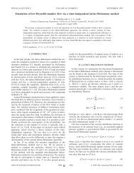
L70 J. Electrochem. Soc., Vol. 138, No. 1, January 1991 9 The Electrochemical Society, Inc.~.0 l,liilll I I'lNlli~ ,liillit-illlill I ,illilll I ,,lilii I lilili, I ililiil I lllilill-Hl'll6,0 -- b a~.oSO07.0- C - ~ I: Theor'etlcal -- l.S_ b: Itilin- l HI6.0 -- C: ~.1, " i0 Ha -- t.25.00.804.08500II1\1 ~ O.,n-O,.,iiit ~ ~176400 / J / ~ d : Umj n - 5.0 Hi3,0 0.4i'~ 200t,0o.o u,r I =Hind ~H~lal IHI,~ ~u,~ ~IHI~ Im~ ~und ~mld ~ml -~.4i0 -~ ~0 -~0 -~ t0 ~ ~0 ~ ~0 ~ ~0 ~ ~104 t0 ~ tO s t07Frequency.Fig. 5. Calculated low-frequency impedance values for the Rondles/CPE electrical circuit of Fig. 2c. This figure illustrates the effect of increasingtruncation frequency, while maintaining the value of r o at10 -z Hz. a, Theoretical impedance response; b, calculated impedancevalues in the frequency range 10 -~ to 1 Hz; c, calculated impedancevalues in the frequency range 10 -3 to 10 Hz; d, calculated impedancevalues in the frequency range 10 -~ to 50 Hz.an indication of the internal consistency of the data set.The polynomial expressions defined in Eq. [A-3] and [A-4],Appendix A, effectively smoothed the scattered impedancedata contained in good-noise. The results for badnoiseshow the calculated impedance below the truncationfrequency to be discontinuous with the experimental dataat r and suggest that bad-noise does not satisfy the KKrelations. The conclusions about the validity of these noisydata sets obtained from the KK algorithm are consistentwith the residual-plot analyses derived from LOMFP.Invalid data sets.---The examples presented in this sectionare for nonstationary systems. Synthetic data weregenerated for the equivalent circuit shown in Fig. 2d bymaking the value of the resistor R, or the capacitor C, varywith time (see the section on simulation of inconsistent independencedata in Appendix B). The "experimental" frequencyrange was 0.1 Hz-65 kHz. Ten data points were collectedper logarithmic decade of frequency and thenumber of delay cycles at each frequency N was six. In-2.5Hz_Ira,, I J lHIII~ IHm, I I BHHI~ J lltll~ J lHI]~ I IHHI~;>.O El, b 8: Theoretical ~mpedanc~_C " ~ b: vei n - 0.5 HZ -,.~ d _ \ o: =.,o . ,.o., -%"~ ~K~ r v.,. SOHzO3Ec" l.O0E o.ep.,io.o _--- i-o.5-I IIl,~ J lHII~ I lllll "l I IIlil~ I lilll ''l I IIIlll~ I nilll~ i ltl,~ III]0 -4 ]0 -~ ]0 -a ]0 -~ ~0 ~ ]0 J ]0 a ]0 ~ 10 ~ t0 sFrequency.Fig. 6. Calculated low-frequency real impedance values for the electricalcircuit of Fig. 2d. This figure illustrates the effect of increasingtruncation frequency, while mointoinlng the value of o~o at 10 -4 Hz. a,Theoretical impedance response; b, calculated real impedance valuesin the frequency range ~0 -~ to O.i Hz; C, coiculated real impedancevalues in the frequency range 10 -4 to 1 Hz; d, calculated real impedancevolues in the frequency range 10 -4 to 5 Hz.Hzo7-zoo ~n~ ~md ,m~,~ ~n~ ~H~ ~lm~ ~n~ ~HH~I ~H~I0 -4 ~0 -s I0 -~ I0 -i I0 ~ lO ~ I0 z ~0 ~ jO 4 IO sFrequency,Fig. 7. Calculated low-frequency imaginary impedance values for theelectrical circuit of Fig. 2d. This figure illustrates the effect of increasingtruncation frequency, while maintaining the value of

= -72 J. Electrochem. Soc., Vol. 138, No. 1, January1991 9 The Electrochemical Society, Inc.Table I, Fitted parameters for the equivalent circuit of Fig, 2d with a variable resistor R~ usingf = 0.0. The nonstotionary systems with various degrees of inconsistency ore givenFP (10). The consistent data set is given forby f = 0.1, 0.175, 0.25, and 0.5f R~, I~ R~, ~ C1, F R~, 12 C~, F Rw, 12 Tw,~0.0 23.22 418.3 1.88E-5 695.2 9.26E-5 846.4 0.70550.100 23.22 419.1 1.87E-5 699.0 9.24E-5 857.3 0.71410.175 23.41 420.2 1.87E-5 701.7 9.22E-5 865.8 0.72040.250 23.48 421.0 1.86E-5 704.3 9.20E-5 874.3 0.72650.500 23.74 423.3 1.84E-5 712.3 9.15E-5 903.73 0.7459two orders of magnitude greater than the other time constants.Acceptable bounds for levels of discontinuity at thetruncation frequency were obtained by comparison tochanges in the calculated values of the circuit parameters.The results are presented in Fig. 16, which illustrates thepercent difference between the values of the circuit elementsfor the stationary and nonstationary systems as afunction of the percent difference between the calculatedand the experimental values for the real impedance at o~,.For these nonstationary systems, a discontinuity of lessthan 15% represents a deviation of less than -+5% for theCircuit elements not associated with the dominant timeconstant. In other words, regression of data showing a 15%discontinuity can be expected to yield circuit parametersassociated with electrochemical reaction rate constantswithin 5% of the values that would apply at the beginningof the experiment. The Warburg component would show alarge error. This establishes an error bounds for the circuitparameters of impedance data sets deemed to be inconsistent.The effect of truncating high-frequency impedance data.-The algorithm incorporated an assumption that the highfrequencyimpedance data have negligible contributionsto the integral when the KK equations are evaluated at lowfrequencies. There is a limit to the truncation of high-frequencydata, however, for this assumption to be valid.Low-frequency impedance values were calculated forthe equivalent circuit shown in Fig. 2d with decreasing(0max. The results are presented inFig. 17. The Bode plotsfor ~om~ = 10 kHz show that the calculated low-frequencyimpedance is continuous with the available data at 0.1 Hz.However, when O~max = 1 kHz, there is a distinct discontinuityat r due to the residual errors at the high-frequencyextreme.The maximum frequency r must be sufficiently largethat the impedance data at the high-frequency range donot truncate in the capacitive region. This requirement canbe relaxed by assuming polynomial expressions for thereal and imaginary impedance in the range to > coax. Additionalsummation terms and polynomial coefficientswould be introduced into Eq. [12] and [13] to account forthe new intervals at the high-frequency extreme.Numerical constraints.--The accuracy of the calculationsis influenced by the choice of the adjustable parametersof the algorithm (see Appendix A). The polynomial ordersK and M must be sufficient to establish the behaviorof the impedance components within the low-frequencyrange; values for K and M between 6 and 10 were deemedto be adequate. As illustrated in Fig. 4, the problem of residualswas minimized by setting coo to be about three orfour orders of magnitude less than COmic. The parameters N~and N~ were specified by dividing the entire frequencyrange into logarithmic decades, and assigning 300 to 1000~i divisions per decade. There was minimal difference betweenthe results obtained when ~i : 1000 and when~ = 300 (note that the optimal value for 8~ can be determinedif an adaptive quadrature method were employed).A noticeable difference was observed when double precision(8-byte floating-point number) was employed as comparedto extended precision (10-byte floating-point number);the discrepancy is due to round-off errors when thesummations are performed.When Nc = 4, N~ = 6, ~i = 1000, and K = M = 9, there are10,000 evenly spaced frequency divisions, and the summationroutine is performed at 20 frequencies within~o0 --- to < O~m~ .. The average computational time required forimplementing the algorithm under these conditions wasapproximately 5 min on a 16 MHz 80386 personal computerwith a math co-processor.ConclusionAn approach has been presented which successfully resolvesthe problem of applying the KK relations to impedancedata which do not exhibit a dc limit. This method differsfrom current KK algorithms such that it does notrequire extrapolation of the experimental data beyond themeasurable frequency domain in order to evaluate the in-300025002000:-~ ~ll.,~ 1.1,~ I J,,,~ i~.l,q I IH,, I ~,,,~ IH,,~ IH_--- ~ a: f - -0. I~,- a " ~ b: f "-0.1751600 30001400 2500t200 2000~ ~ ~ ~ F T ~ ,s00- --- 14oof - to-Sb: f - 5xi0-s ..-~_- ,200t500~ t000500d: f - -0.51000 t500.00 g g ,ooooo0~ ~ 6OO .0_zo,.,400 0400-500-lO00-t500~ . -zl i,.,) o:llIlll~ [Itllill~ IIIIII,] llilfilll flfllll~ IIIIII~ lllfll~ lIIll(d lllf -2oo10 -4 1.0 -s :10-2 10 -t iO 0 ~0 t :10 a 10 3 10 4 :105Frequency.Fig. 13. Calculated low-frequency impedance values for a simulatednonstationary system in the frequency range 10 -4 to 0.1 Hz. The electricalcircuit of Fig. 2d was used with a variable resistor R~ and negativevalues of "inconsistency factor" f. The value of the resistor decreasedduring the course of the "experiment." Curve a: f=-0.1(AR1 =--7.0%), b: f=-0.175 (AR~ =-12.2%), c: f=-0.25(ARI = - 17.4%), d: f = -0.5 (~R1 = -35.0%).Hz200 -500-t000-1500:lL.,~ i i.,d ,..ll i.,Id ~Hml i.,id J.l,d I.,~ i.t~ -~ooI0 -4 I0 -3 i0 .2 I0 -I I0 ~ IO ~ :10 2 10 3 I0 4 IO SFrequency,Fig. 14. Calculated low-frequency impedance values for a simulatednonstationary system in the frequency range 10 -4 to 0,| Hz. The electricalcircuit of Fig. 2d was used with a variable capacitor CI and positivevalues of "inconsistency factor" f. The value of the capacitor increasedduring the course of the "experiment." Curve a: f = 10 -s(ACI= 15.5%), b: f=5• 10 -s (AC1=77.5%), c: f= 10 -7(ACI = 155%).Hz200o

J. Electrochem. Soc., Vol. 138, No. 1, January 1991 9 The Electrochemical Society, Inc. 73,ooo \ , ,._o,o,80060040O2500 ~1 lillll~ t lllllll t I III111~ I IIIIIll I I llllJl~ I lliJllJ] I IH(J~I~-[~_ eoo2000 ~-.~. a /'~ a: =...- to k,z -.... .'.'.'.'.' :::::: soo-- b b: ula I = | kHzA500~ooo ~ c k500ozr (w)-200-400~N.;~~- 2oo N5000I-soo -~ u)H)~ ~ u).l,l I.II)~ )))ud ))I))l~ I I)))Ig I I)~),~ luI.~ )I)I~ -~oo~0 -( 1.0 -3 10 -2 ~0 -~ ~.0 ~ iO ~ ~0 ~ I0 ~ i0 ( I0 sFrequency, HzFig. | 5. Calculated low-frequency impedance values for a simulatednonstationary system in the frequency range 10 4 to 0.1 Hz. The electricalcircuit of Fig. 2d was used with a variable capacitor C~ and negativevalues of "inconsistency factor" f. The value of the capacitor decreasedduring the course of the "experiment." Curve a: f = -10 -e(AC1 = -15.5%), b: f = -5 x 10 -~ (ACI = -77.5%), c: f = -10 -7(AC) = - 155%).-~ooHllliJ ~ulll)l l llllll~ l lu,,I l lll,l~ luIlIl~ luI,d l ltll~ -2oo~0 -4 ~,0 -3 ~,0 -2 iO -1 iO ~ ~01 iO 2 10 3 iO 4F'requency, HzFig. 17. The effect of decreasing O)ma x on the algorithm attributableto the problem of residuals at the high-frequency extreme. The datasets were from the equivalent circuit of Fig. 2d and co,~, = 0.1 Hz.Curve a: C%ax = 10 kHz; and b: O)ma x = 1 kHz. a, Calculated impedancevalues in the frequency range 10 -4 to 0.1 Hz when~0=~ = 110 kHz; b, calculated impedance values in the frequencyrange 10 -4 to 0.1 Hz when (Oma x = 1 kHz.tegrals of the KK relations. The proposed technique usesonly the available impedance data, which is necessarilyconstrainted within a finite frequency domain. The onlyrequirement for testing the consistency of the data usingthe method presented in this paper is that the highestmeasured frequency should be large enough to ensure thatthe high-frequency impedance data do not terminate inthe capacitive region.This KK algorithm should facilitate the analysis and interpretationof experimental data. This procedure complementsthe method of fitting impedance data to an equivalentcircuit; in part because a fitting procedure can be atedious and time consuming exercise. By first appl~-ing theKK algorithm, an experimenter will know whether thedata are suitable for analysis by a fitting procedure. If theexperimental data is found to satisfy the KK relations,then an equivalent circuit could be found which will providea "good" and acceptable fit. Otherwise, the experimenterwill be aware of the inconsistency of the data set,and should interpret the results of the fitting procedure inlight of a possible violation of one of the conditions of theKK relations.AcknowledgmentsThis material is based upon work supported by the NationalScience Foundation under Grant no. EET-8617057and on work supported by DARPA under the Optoelectronicsprogram of the Florida Initiative in Advanced Microelectronicsand Materials. The writers also wish to acknowledgethe contributions of Conrad B. Diem.Manuscript submitted Jan. 15, 1990; revised manuscriptreceived Aug. 2, 1990.i01I i I I I I IlJ I I IoAPPENDIX AAlgorithm far Calculating Low-Frequency ImpedanceThe two forms of the KK relations (3, 7) employed in thisalgorithm wereZi(r = - 10 x---- ~-_ w~ dx [A-l]uCL2q--4~C0JUr0Jn10 ol0 -s~0 ~ 2 3II&B I/AAW= ~ Z~t SYNBOLS --o R w 9 T N0 FIt o C!,~ R 2 ~ C 2v R sI I I IIII I I I4 5 6 7 eg ~.01 2 3 4 5} Zr. expt - Zr. calc I /Zr. expt * :iO02 r| xZi(x) - coZi(~)z~(~o) : Z~(| + ~ ~o/ -~ --~ dx [A-2]Zr(r and Zi(r are the real and imaginary components ofthe impedance, and r and x are angular frequencies. Equation[A-l] represents the imaginary impedance that is internallyconsistent with the real component of the experimentaldata. Equation [A-2] represents the real impedancethat is internally consistent with the imaginary componentof the experimental data.Based on the assumptions presented in the section onConcept, the infinite integration region for the KK equationsis limited to r -< x -< r Experimental data wereassumed to be available for the frequency ranger --< X --< COmax; the real component reaches an asymptoteZr| and the imaginary component approaches zero at ~0max.The object of the algorithm was to determine the functionsfor the real and imaginary componentsFig. 16. The effect on inconsistency on the calculated parameters ofthe equivalent circuit of Fig. 2d. The abscissa represents the percentdifference between the real component of the data set and the calculatedreal impedance at con. The ordinate is the percent different betweenthe values of the circuit elements of the nonstationary and stationarysystems.KZr(oJ1) = ~ a(k l) (log ~o~) k [A-3]k=0MZi(00,) = • a~ )(log to,) m [A-4]m=O

74 J. Electrochem. Soc., Vol. 138, No. 1, January 1991 9 The Electrochemical Society, Inc.within the low-frequency range r

J. Electrochem. Soc., Vol. 138, No. 1, January 1991 9 The Electrochemical Society, Inc. 75match the set of polynomial coefficients for both equations where[for example, see algorithm 7.4, Ref. (16)].This iterative routine may be avoided by using Eq. [A-12]ftand [A-13] simultaneously when constructing the linearhsystem of(K + M + 2) equations. For example, Eq. [A-12] isZemployed when l is odd, and Eq. [A-13] when I is even. Thishdirect method yields polynomial coefficients that are validfor both equations and which result in residuals of compa-Prable orders of magnitude. This was the approach taken inKthe calculations presented in this paper. The computerprogram to implement the algorithm was written in TurboPascal (Boriand International, Version 5.0) and compiled ~2in math mode. The gaussian elimination routine with ~1scaled-column pivoting (16) and the Simpson's rule routinewere performed using 80 bit "extended" floating-point 0-numbers to minimize round-off errors.APPENDIX BTheoretical Impedance ExpressionsThe analytic expressions employed for calculating theimpedance response of the equivalent circuits depicted inFig. 2 are listed in this section.Circuit 2a.--The real and imaginary impedance componentsfor the Randles circuit of Fig. 2a were calculatedfromZT(tO ) = Zr(~ ) + jZi(tO)= R~+ 2 s 2 -J" z 2 s1+ tO R1C 1 1 + (o R1C 1[B-l]Circuit 2b.--The impedance response for the Randlescircuit with a Warburg impedance shown in Fig. 2b is deconvolutedfrom the impedance response of the electricalcircuit of Fig. 2d by reducing the value of the time constantR2C2. Consequently, the impedance data are calculatedfrom Eq. [B-6] presented in the following section onCircuit 2d by setting the values of R2 and Cs equal to zero.Circuit 2c.--The electrical circuit of Fig. 2c was used tomodel the impedance behavior of mild steel in concentratedhydrochloric acid (17). It has a constant phase element(CPE), whose impedance is given by1ZCPE -- - - [B-2]Yo(JtOPThe rationale behind the use of this element is discussed inRef. (18), Since= pZ - ,ha= pA - ,z= coClp= K - ~C1@= Rw~l~ - d0eR2v2~= R1K + RwX~ + 6~R2= 6 ~= 1 + ~2~= 8 2 d- 0 -2= RsC2= ~/~ sin 6 - ~0- cos 4~= ~ cos ~0 + ~/0- sin 6= ~ sin O~ + ~/cos ~b= ~ cos 4~ - ~ sin= e* + e-*: e @ -- e-~2V~Y~Tw2Simulation of inconsistent impedance data.--Inconsistentimpedance data for a nonstationary system were simulatedby changing the value of a circuit element duringthe course of the "experiment." A simple case is to assumethat the value of the circuit element E varies proportionallywith time. ThereforeiEi = Eo + fN ~ ht~n-1[B-7]where Eo is the value of the circuit element at start of theexperiment, i is the number of data points collected, and Eiis the value of E as the experiment progresses. The "inconsistencyfactor" f accounts for the direction of change of E;the value of E decreases with time when f < 0, and increaseswhen f> 0. N represents the number of cyclesused to make measurement at a given frequency. The timerequired to complete one cycle is ht = 1/~0, and NAt = N/tocorresponds to the total time which has elapsed when themeasurement was performed. The expression for Ei becomeszEi = Eo + )~ E --1n-1 tOn[B-8]where tO1 = 65 kHz since impedance experiments are usuallyperformed from 65 kHz down to low-frequency values.The percent difference between the initial value of the circuitelement and its value at any time during the "experiment"is given bythe analytic expression for this equivalent circuit is( ctR1 ) ~R1Zw(a) = Zr(cO) + jZi(~) = R~ + a s + B -T - j az + B2 [B-4]where~ = l+YoRltOncos(~)=YoRlto~sin(~)Circuit 2d.--The equivalent circuit of Fig. 2d was employedto model the impedance response of copper dissolutionin alkaline chloride solutions (19). The expressionemployed for the Warburg impedance Zw is given by (14)tanh (X/jtOTw)Zw = RwVj~Tw[B-5]The analytic impedance response of the equivalent circuitshown in Fig. 2d isZr(tO) = Z~(tO) + jZ~(~)= R~+ A2+N2 - j hs+Z~ [B-6]Ei - Eo fN ~ 1hEro - - - • 100 = ~ -- • 100 [B-9]EoEo ,,=1 tOnEquation [B-8] was used to calculate the values of a variableresistor or variable capacitor, and was incorporatedinto the analytic expressions listed above to simulate anonstationary system. The value of N was set to 6 whengenerating the inconsistent data sets.REFERENCES1. R. L. Van Meirhaeghe, E. C. Dutoit, F. Cardon, andW. P. Gomes, Electrochim. Acta, 29, 995 (1975).2. D. D. Macdonald and M. Urquidi-Macdonald, ThisJournal, 132, 2316 (1985).3. M. Urquidi-Macdonald, S. Real, and D. D. Macdonald,ibid., 133, 2018 (1986).4. R. de L. Kronig, J. Opt. Soc. Am. Rev. Sci. Instrum., 12,547 ((1926).5. H. A. Kramer, Phys., Zeits., 31), 522 (1929).6. B. Davies, "Integral Transforms and Their Applications,"Applied Mathematical Series, Vol. 25, 2nded., Springer-Verlag, New York (1985).7. H. W. Bode, "Network Analysis and Feedback AmplifierDesign," D. Van Nostrand Co., Inc., New York(1945).8. D. D. Macdonald and M. Urquidi-Macdonald, ThisJournal,137, 515 (1990).9. H. Shih and F. Mansfeld, Corros. Sci., 28, 933 (1988).10. H. Shih and F. Mansfeld, in "Transient Techniques inCorrosion Science and Engineering," (PV89-1)W. H. Smyrl, D. D. Macdonald, and W. J. Lorenz, Ed-

76 J. Electrochem. Soc., Vol. 138, No. 1, January 1991 9 The Electrochemical Society, Inc.itors, p. 31, The Electrochemical Society SoftboundProceedings Series, Pennington, NJ (1989).11. H. Shih and F. Mansfeld, Corrosion, 45, 325 (1989).12. D. D. Macdonald and M. Urquidi-Macdonatd, ibid., 45,327 (1989).13. M. C. H. McKubre, D. D. MacDonald, and J. R. Macdonald,in "Impedance Spectroscopy: EmphasizingSolid Materials and Systems," J. R. Macdonald, Editor,p. 180, John Wiley & Sons, Inc., New York(1987).14. J. R. Macdonald, "Complex Nonlinear Least SquaresImmittance Fitting Program: LOMFP," Universityof North Carolina, Chapel Hill, NC.15. K. Ohta and H. Ishida, AppL Spectros., 42, 952 (1988).16. R. L. Burden and J. D. Falres, "Numerical Analysis,"4th ed., Prindle, Weber & Schmidt, Boston, MA(1989).17. F. B. Growcock and R. J. Jasinski, This Journal, 136,2310 (1989).18. J. R. Macdonald, J. Anal. Chem., 223, 25 (1987).19. O. C. Moghissi, MS Thesis, University of Virginia,Charlottesville, VA (1989).The Effect of Tungsten on the Corrosion Behavior of AmorphousFe-Cr-W-P-C Alloys in 1M HCIHiroki Habazaki, Asohi Kawashima, Katsuhiko Asami, and Koji HashimotoInstitute for Materials Research, Tohoku University, Sendai 980, JapanABSTRACTThe active current density of Fe-8Cr-7W-13P-7C alloy is almost three orders of magnitude lower than that of theFe-8Cr-13P-7C alloy. The passive current density in the low potential region also decreases with increasing alloy tungstencontent. The surface analysis by XPS reveals that chromium and tungsten ions are concentrated in the surface film on atungsten containing alloy in the active region. The thickness of the surface film formed on the low tungsten alloy in theactive region is x-ray photoelectron spectroscopically infinite, whereas the film thickness on the Fe-SCr-7W-13P-7C alloyin the active region is of the same order of magnitude as the thickness of the passive film. The chromium enrichment in thepassive film becomes more significant with increasing tungsten content. Passivation of low tungsten alloys seems to occurby the formation of the passive film with the least enrichment of chromium ions necessary for passivation due to differentdissolution rates of iron and chromium during a large amount of alloy dissolution. Passivation of tungsten containing alloystakes place through transformation of the air-formed film to the passive film as a result of preferential dissolution of asmall amount of iron without dissolution of chromium ions.It is well known that amorphous metal-metalloid alloyswith a certain amount of chromium have extremely highcorrosion resistance in neutral and acidic solutions (1-8).Such a high corrosion resistance of amorphous alloys hasbeen thought to be due to their chemical homogeneity andhigh passivating ability of amorphous alloys (3): amorphousalloys are free of defects such as grain boundariesand dislocations, and of compositional fractuation formedby solid-state diffusion, Such a chemical homogeneity assiststhe formation of a uniform passive film on amorphousalloys. The high chemical reactivity of amorphous alloys ispartly based on the existence of many coordinatively unsaturatedatoms which enhances dissolution of elementsunnecessary for the formation of the passive film. Rapiddissolution of such elements is responsible for the highpassivating ability due to rapid surface concentration ofions, such as chromic ions, necessary for passive film formation.The addition of molybdenum to amorphous iron-chromium-metalloidalloys further improves the corrosionresistance (4-8). When sufficient amounts of chromium andmolybdenum are added, the amorphous iron-metalloid alloyspassivate spontaneously even in hot concentrated hydrochloricacid (5-8). It is also well known that the additionof molybdenum to stainless steels increases the corrosionresistance, especially resistance to occluded cell corrosion(9-11).Some of the present authors have carried out the analysisof surface films on amorphous and crystalline iron-basealloys containing chromium and molybdenum by x-rayphotoelectron spectroscopy and attempted to clarify therole of molybdenum in increasing the corrosion resistance(7, 8, 12). It has been revealed from these investigationsthat in the active region, molybdenum ions are remarkablyenriched in a surface film but not in the passive film andthat the passive film is composed mostly of hydrated chromiumoxyhydroxide. They proposed a possible role of molybdenumin assisting the formation of the passive hydratedchromium oxyhydroxide film by considering theanalytical data as well as passivation kinetics.The beneficial effect of tungsten has been known formany years. For example, tungsten improves resistance topitting corrosion of stainless steels in chloride media(14, 15). Like molybdenum, the addition of tungsten improvesthe corrosion resistance of amorphous Fe-P-C alloyswith and without chromium in hydrochloric acid(4, 13). However, its effect in improving the corrosionresistance is not sufficiently understood yet.This work has been performed to clarify the beneficialrole of tungsten on the corrosion behavior of amorphousFe-Cr-W-P-C alloys in hydrochloric acid by combination ofelectrochemical methods and x-ray photoelectron spectroscopy.ExperimentalFe-xCr-yW-13 atom percent (a/o) P-7 a/o C (x = 4, 6, and8 a/o; y = 0, 1, 2, 3, 5 and 7 a/o) alloy ingots were preparedby high-frequency induction melting of laboratory madeiron phosphide and commercial iron carbide, tungsten,chromium, and iron under an argon atmosphere. Ironphosphide was prepared by sintering red phosphorus iniron. From these ingots, amorphous alloy ribbons of about1 mm width and 10-30 ~m thickness were prepared by asingle-roller method. X-ray diffraction patterns of the alloyswere measured with the x-ray diffractometer using CuKs radiation. All of the specimens used showed only halopatterns characteristic of amorphous structure.Prior to electrochemical measurements, the amorphousalloy ribbons were polished in cyclohexane with siliconcarbide paper up to no. 1000, degreased ultrasonically inacetone and dried in air. Electrochemical measurementswere carried out at 303 K in deaerated 1M HC1 solutionwhich was prepared from a reagent grade chemical and deionizedwater. Potentiodynamic polarization curves weremeasured with a potential sweep rate of 143 mV min-L Potentiostaticpolarization was carried out for lh at variouspotentials by using different specimens to get differentpoints in potentiostatic polarization curves. After the potentiostaticpolarization or immersion for lh, these specimenswere washed in water and dried in air, and then they