THE PATCH-CLAMP TECHNIQUE EXPLAINED AND EXERCISED ...

1. INTRODUCTION1.1. What is patch clamping?When one hears the words "patch-clamp" or "patch-clamping" for the first time in the scientificcontext, in which this term is so often used (cell physiology and membrane electrophysiology), itsounds like magic or silly jargon. What kind of patch, clamp or activity is one talking about?Obviously, not clamping patches of material together as one might do in patchwork or quilting!"Patch" refers to a small piece of cell membrane and "clamp" has an electro-technical connotation.Patch-clamp means imposing on a membrane patch a defined voltage ("voltage-clamp") with thepurpose to measure the resulting current for the calculation of the patch conductance. Clampingcould also mean forcing a defined current through a membrane patch ("current-clamp") with thepurpose to measure the voltage across the patch, but this application is rarely used for small patchesof membrane. Thus, since the introduction of the patch-clamp technique by Neher and Sakmann in1976, patch-clamp most often means "voltage-clamp of a membrane patch.” Neher and Sakmannapplied this technique to record for the first time the tiny (pico-Ampere, pA, pico = 10 -12 ) ioncurrents through single channels in cell membranes. Others had measured similar single-channelevents in reconstituted lipid bilayers. However, the patch-clamp technique opened this capability toa wide variety of cells and consequently changed the course of electrophysiology. That was, at thattime, an almost unbelievable achievement, later awarded the Nobel Prize [see the Nobel laureatelectures of Neher (1992) and Sakmann (1992)].This accomplishment, and the quirky name of the technique, no doubt added to the magical soundof the term patch-clamp. Remarkably, the mechanical aspects of the technique are as simple asgently pushing a 1 µm-diameter glass micropipette tip against a cell. The membrane patch, whichcloses off the mouth of the pipette, is then voltage-clamped through the pipette from theextracellular side, more or less in isolation from the rest of the cell membrane. For this reason thepatch-clamp amplifiers of the first generation were called extracellular patch-clamps.1.2. Five patch-clamp measurement configurationsNeher and Sakmann and their co-workers soon discovered a simple way to improve the patchclamprecording technique. They used glass pipettes with super-clean ("fire-polished") tips infiltered solutions and by applied slight under-pressure in the pipette. This procedure caused tightsealing of the membrane against the pipette tip measured in terms of resistance: giga-Ohm sealing,giga = 10 9 . This measurement configuration is called cell-attached patch (CAP) (see Fig. 1.1),which allowed the recording of single-channel currents from the sealed patch with the intact cellstill attached. This giga-seal procedure allowed Neher and Sakmann and their co-workers to obtainthree other measurement configurations, including one for intracellular voltage- and current-clamp:the membrane patch between the pipette solution and the cytoplasm is broken by a suction pulsewhile maintaining the tight seal (Hamill et al., 1981). In this so-called whole-cell (WC)configuration (Fig. 1.1), the applied pipette potential extends into the cell to voltage-clamp theplasma membrane. Alternatively, the amplifier could be used to inject current into the cell tocurrent-clamp the cell membrane and to record voltage, for example to study action potentials ofsmall excitable cells, which was impossible until the development of the giga-seal. Another3

achievement of the WC-configuration was the possibility to perfuse the intracellular compartmentwith the defined pipette solution. Although the WC-clamp configuration is no longer a clamp of asmall membrane patch, electrophysiologists continued to refer to the WC-clamp configuration as avariant of the patch-clamp technique, probably because the WC-clamp starts with giga-sealing asmall membrane patch.Two other variants are inherent to the patch-clamp technique, since they concern clamping a smallarea of membrane. The giga-seal cell-attached patch, sometimes called an "on-cell" patch, can beexcised from the cell by suddenly pulling the pipette away from the cell. Often the cell survives thishole-punching procedure by resealing of the damaged membrane, so that the excision can berepeated on the same cell. The excised patch is called an inside-out patch (IOP) (Fig. 1.1),because the inside of the plasma membrane is now exposed to the external salt solution. Thisconfiguration allows one to expose the cytoplasmic side to defined solutions in order, for example,to test for intracellular factors that control membrane channel activity. Another type of excisedpatch can be obtained, but now from the WC-configuration rather than the cell-attachedconfiguration. It is the outside-out patch (OOP), which is excised from the WC configuration byslowly (not abruptly now!) pulling the pipette away from the WC (Fig. 1.1). This maneuver firstdefines a thin fiber that eventually breaks to form a vesicle at the tip of the pipette. Theconfiguration obtained is indeed a micro-WC configuration, which allows one to study smallpopulations of channels or single channels and to readily manipulate the “tiny cell” to differentbathing solutions for rapid perfusion.The connection of the current (I) or voltage (V) measuring amplifier to the pipette and the bath isshown in Fig. 1.1 for the OOP, but this connection applies to all other configurations as well. Themeasuring electrode is inserted in the pipette, while the reference electrode is in the bath. Theresulting circuit is shown for the recording of a single OOP channel current, driven by an intrinsicvoltage source in the channel and/or a voltage source in the amplifier. The fifth configuration is thepermeabilized-patch WC-configuration (ppWC) (Fig. 1.1), in which the CAP is not actuallyruptured for direct access to the inside of the cell, but made permeable by adding artificial ionchannels (monovalent cation channel-forming antibiotics) via the pipette solution (Horn and Marty,1988). Examples of such antibiotics are amphotericin and nystatin, both produced bymicroorganisms. The great advantage of this configuration is that it allows intracellular voltageandcurrent-clamp measurements on relatively intact cells, i.e. cells with a near normal cytoplasmiccomposition. This is in contrast to the perfused WC-configuration. The various patch-clampconfigurations are beautifully described in Neher and Sakmann (1992).It is the purpose of the present contribution to make the beginning student familiar with theelectrophysiological procedures involved in experimenting with each of the five patch-clampconfigurations. The required theoretical background will be provided and the explained theory willbe exercised with patch-clamp experiments on a model cell designed for teaching and testingpurposes.4

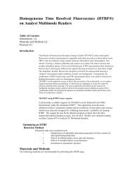
Figure 1.1. Diagram of the five patch-clamp measurement configurations. The figure depicts a living cell seenfrom the side immersed in extracellular solution and adhered to the substrate. The barrel-type pores in the membrane(some with movable lids or gates) represent ion channels. The five “cups” drawn in semi-perspective close to the cell arethe tips of fluid-filled glass micro pipettes connecting the cell to the amplifier. The figure is a composite drawing, as ifall five pipettes were placed on one cell. Although this is not a practical possibility, it is possible to make simultaneoustwo-electrode WC/CAP recordings (see elsewhere in the present book) and CAP/CAP would not be out of the question.All five tips are in position to illustrate how the various measurement configurations are derived from the initial cellattached-patch(CAP) configuration, established after the giga-sealing procedure. The inside-out patch (IOP) is a CAPexcised from the cell membrane. The whole-cell (WC) configuration is obtained by rupturing the CAP. The outside-outpatch (OOP) is a vesicle (a “tiny cell”) pulled from the WC configuration. The permeabilized-patch WC (ppWC)develops from the CAP if the pipette solution contains pore-forming molecules incorporating in the CAP. Themeasuring patch-clamp amplifier and the connecting electrodes, one inside the pipette and one in the bathing solution,are drawn for the OOP-configuration. However, they apply to the other configurations as well. The amplifier measurescurrent (I) through the membrane or voltage (V) across the membrane.1.3. Why use electrical equivalent circuits?Patch clamping is an electrical technique, which requires some skill in electrical thinking andmeasuring. When a patch-clamper is going through the procedures to obtain one of the fivemeasurement configurations, he or she is continuously monitoring voltage-step induced current5

esponses or current-step induced voltage-responses to check whether the procedures work. Whiledoing that, the experimenter is also continuously conceptualizing the measurement condition as asimple electrical circuit model consisting of resistors (R), capacitors (C), and batteries (E). Becausethese models are nearly equivalent to the real measurement conditions in certain (but not all!)respects, these models are also called equivalent circuits.Examples of this way of testing and proceeding are illustrated in Fig. 1.2a. The patch-clamp (pc)amplifier is here represented by a voltage source, Epc, in series with a resistor, Rpc, both shunted byan input capacitance, Cpc. The measuring patch pipette can be represented by the pipette resistance,Rpip, and pipette capacitance, Cpip, as soon as the pipette enters the solution. Giga-sealing thepatch pipette to the cell membrane can be represented by replacing the direct connection of thepipette with the grounded bath by the seal resistance Rseal. After forming the giga-seal, the pipetteopening is closed off by the cell-attached patch (CAP) with its high resistance, Rcap. Breaking theCAP replaces Rcap for access resistance, Racc, providing access to the inside of the whole-cell(WC) with its Em:Rm:Cm membrane.Fig. 1.2b shows that the three steps in the procedure for obtaining a WC-configuration can besimulated by a simple ERC-circuit with three switches (S). Closure of Spip (double switch withScpip and Srpip) would represent entering the bath with the pipette, opening the switch Ssealsymbolizes (abrupt) sealing, and closure of switch Sacc simulates WC-establishment by shortcircuiting Rcap with the access resistance Racc. During actual experiments the experimenter canrecognize entering the bath, giga-sealing the cell and making a WC by applying voltage steps in Epcto the pipette and interpreting the current responses as if the circuit of Fig. 1.2b applies. This is themain value of equivalent circuits. The same is true for obtaining the other three patch-clampconfigurations discussed above (IOP, OOP, ppWC). Thus, thinking in terms of simple ERCcircuitsis essential for readily doing the tests and subsequent experiments. Therefore, studentsinterested in learning patch clamping should begin to familiarize themselves with this way ofthinking and measuring.6

Figure 1.2. A simple electrical circuit modeling the successive patch-clamp procedures for obtaining the wholecellconfiguration. A pipette (PIP) entering the bath, forming a giga-seal with the cell, and breaking the cell-attachedpatch. Part a shows how the various components of the circuit can be identified with components of the measurementconfiguration(s). Part b shows the circuit abstracted from the drawing in Part a, including the switches (S) for goingthrough the three successive procedures leading to a WC configuration. The procedures and component names arefurther explained in the text. During the experiment the quality of the pipette, the giga-seal, and the whole-cellconfiguration are tested by applying voltage-clamp Epc steps to the pipette and measuring the resulting patch-clampcurrent Ipc.7

But how? Studying electronics (Horowitz and Hill, 1990) will help, but this may be an unwanteddetour for those students ready to do the experiments. Many electronics courses and textbooks alsodiscuss the properties of inductors, transistors and operational amplifiers, while these subjects arenot of major importance for the beginning or even the advanced student in electrophysiology. Inour opinion, mastering ERC-circuits should have the highest priority for obtaining measurementskills. The earlier chapters of the present book are particularly devoted to providing the basics ofbioelectricity to the beginning student and attempts to fill the gap between basic physical theory andmore advanced membrane electrophysiology textbooks (Hille, 2001).After the present introduction, we begin with the theory of the basic ERC-circuits relevant for patchclamping. Since patch clamping is a technique often used in multi-disciplinary teams of biomedicalscientists, students from biology or medicine often want to learn the technique. As they frequentlydo not have much background in physics or electronic technology, it may be helpful if such studentshave biological examples of the physics they are learning. Such examples are usually not providedin the general electronics courses. Here we take the opportunity to give such examples whileexplaining the theory. Fig. 1.2 already shows several important models and the earlier chapters ofthe present book should help provide the physical basics of ERC components and circuits. Westress, however, that whatever the importance of the theory, practical exercises are as important.Biophysics is an experimental science and trying to recognize ERC-circuit behavior in the electricalbehavior of a real circuit or in a living cell is of great instructive value.Manuals for practical classroom courses on the electronics of ERC-circuits for patch-clamp studentsare available (Ypey, 1997). However, the most attractive way to become introduced to patchclampingis to exercise the theory in a real patch-clamp set-up on an equivalent circuit model of acell showing all the relevant ERC-behavior of a living cell, i.e., with realistic E, R and C values.That is what we do in Chapter 3. It allows the student to combine learning the theory withbecoming familiar with a practical set-up. It also forces the student to identify components of apatched cell with electric circuit components (E, R or C). Students ready to start patch clampingmay use Chapter 3 as an instruction manual for how to test a set-up in preparation for actualexperiments. Reading Chapter 3 before beginning experiments will serve the student more thanmerely reading the instruction manual of a patch-clamp amplifier, although that should not beforgotten!To our knowledge, a structured patch-clamp measurement exercise course as presented here hasnot yet become available for general use and teaching. This is in contrast to the many computerprograms available for teaching concepts of biophysical or physiological mechanisms. Althoughthese teaching models may be invaluable, in particular for patch-clampers, they do not providepractical measurement exercises. The latter are important because measurement conditions alwayspresent practical problems that must be solved before one is able to make sense of the observations.There are, of course, limitations to the model exercises presented here. One is the lack of "wet"(i.e., physical-chemical) properties in the ERC-circuit cell model. Also there is no opportunity toencounter and solve electrode offset or junction potential problems, or to study the ionic dependenceof membrane potentials. These topics must be dealt with separately. Another shortcoming of theERC cell model one should notice is that it lacks Hodgkin-Huxley “excitability” conductanceproperties. That would be useful, but once able to make reliable measurements, the student will find8

that Hodgkin-Huxley teaching models for conceptual training (e.g. Neuron, Ref?, see alsoPlenumBTOL) are available for further exercises and experiments. A book of great practical use inall aspects of the patch-clamp technique is The Axon Guide of Sherman-Gold (1993).A final comment on limitations: the ERC-circuit with a voltage source Es in series with an internalsource resistor Rs (thus two connection terminals) only applies to patch-clamp stimulation (voltageclamp or current clamp) because the patch-clamp is a true two-terminal input, single-electrodeclamp. Although the approach in principle also applies to three-terminal, two-microelectrodevoltage-clamp stimulation, this would require some rethinking and redrawing of the measurementconfigurations. Further justification for using ERC-circuit equivalents in electrophysiology is givenin PlenumBTOL.9

2. FOUR BASIC ELECTRICAL EQUIVALENT CIRCUITSIn the present chapter we discuss the properties of four simple electrical circuits representing sixfrequently encountered experimental conditions during patch clamping. For practical and didacticreasons, we discuss these successively as circuits of increasing complexity. Nevertheless, thedifferent situations are rather similar and reduce to two types of basic circuits in many applications,one with one capacitor and the other with two. The simplest circuit, the first one, is most frequentlyemployed during practical experiments. Here it is also used to introduce and explain the equations(Ohm's Law, Kirchoff's Law, and capacitor equation) that describe the behavior of all four circuits.The circuits are denoted as ERC-circuits, since they contain batteries (E), resistors (R) andcapacitors (C). When introducing the circuits, we will indicate in which respect these circuits canserve as equivalents of practical patch-clamp configurations. The practical use of these circuits willbecome apparent in demonstrations on the model cell in Chapter 3. Where appropriate, we willdiscuss important properties of the circuits for real patch-clamp experiments.Discussion of the four ERC-circuits will serve as preparation for the demonstrations. The theory ofthe four practical circuits is so important that one can hardly imagine doing patch-clampexperiments without understanding this theory. The circuits will also be used to explain thedifference between voltage-clamp and current-clamp stimulation. Although these two stimulationtechniques are methodologically very different, technically speaking they are only extremes of oneand the same technique. It is very important that the student becomes fluent in switching fromvoltage-clamp to current-clamp thinking. Some electrophysiologists may rely too heavily on onlyvoltage-clamp, even though voltage-clamp was designed primarily to understand the unclampedbehavior of excitable cells. The ERC-circuit approach used here is an excellent way to integrateboth ways of clamping in one framework. In a later stage of learning patch-clamp, this approachwill help to understand and identify bad voltage-clamp recordings from excitable cells.2.1. Charging a capacitor: ERC circuit IFig. 2.1a gives the most simple battery-resistor-capacitor (ERC) circuit (ERC-circuit I) one canconceive, because it consists of only one battery (Es), one resistor (Rs) and one capacitor (C), allthree components in series in a closed circuit. The index ‘s’ (which stands for ‘source’) indicatesthat we consider the Es:Rs combination as a source that provides the current to charge C. Thissource may be a voltage- or current-clamp instrument, and C may be the capacity of the patchclampinput, of a patch pipette or of the membrane of a cell, as illustrated in Fig. 1.2. Before thepipette touches the bath, Epc, Rpc, and Cpc form the ERC-circuit I. After forming a giga-seal, Epc,Rpc, and Cpc + Cpip again form ERC-circuit I if Rseal and Rcap are very large. In the whole-cellEpc, Rpc + Rpip + Racc and Cm may form ERC-circuit I, if Rm and Rseal are very large and Cpc+ Cpip very small.10

Figure 2.1. Charging a capacitor: ERC-circuit I. Part a shows the ERC-circuit studied, b the voltage-clampbehavior upon an Es voltage step at a given (low) value of Rs and c the current-clamp behavior of the circuit upon amuch higher Es voltage step at a much higher value of Rs (notice time calibration difference). The upper records ofb and c show the Es voltage steps applied (positive, from zero) and the exponential Vc responses. The lower recordsshow the exponential current responses. Notice that the Vc and Irs transients change with the same time constantsand that the current-clamp transients are much slower than the voltage-clamp transients. In both cases there is nostationary current after the transient, since Vc becomes exactly equal to Es. Es is the stimulating voltage, Irs is thecurrent through the source resistance Rs, Vc is the voltage across the capacitor C, and Ic is the current flowing intoC. The records in panels b and c have been calculated with the use of a computer model of the circuit in a for thecomponent values given in panels b and c.Here we want to understand how steps in the voltage Es, as occur during patch-clamp experiments,charge the capacitor: how rapidly is C charged, by which current, and to what voltage? Weconsider step changes in Es rather than other functions, such as sinusoidal or ramp functions,because step changes are widely used in electrophysiology for membrane stimulation.Electrophysiologists often study how membrane conductance changes when the voltage changesabruptly to a new, fixed value because this is simple to analyze. A quick way to do that is byapplying a step change in potential.We need three equations as mathematical tools to describe the behavior of circuits like Fig. 2.1 (formore theoretical background, see the earlier chapters of the present book). The first formula isOhm's law, V = RI, which relates the voltage V (expressed in units of volts, with V as thesymbol), across a resistor R (in units of ohms, with Ω as the symbol) to the current I (in units of11

amperes, with A as the symbol) flowing through the resistor. You may think of R as proportionalityconstant between V and I.It is convention in membrane electrophysiology to define intracellular voltage and membranecurrent polarity with respect to the ground ( = arbitrary ‘zero’ voltage) on the external side of themembrane. Thus the ground symbols in Figures 2.1-4 indicate the external side of a membrane ifthe circuit is taken to represent stimulation of a cell with the Es&Rs source. Voltage sources arethen positive, if the positive side of the battery is facing the inside of the membrane. Membranecurrents are positive when they flow from the inside to the outside, driven by a net positive voltagedifference across the membrane.In our derivations we will often choose positive voltage sources and consider a consistent path ofcurrent flow, but the resulting equations will describe voltages and currents for any voltage polarity.For ERC-circuit I, Ohm's law impliesorVrs = Es - Vc = Rs IrsIrs = (Es - Vc) / Rs(1a)(1b)with Vrs the voltage across Rs, Es the source battery voltage, Vc the voltage (difference) across thecapacitor C and Irs the current through Rs. This equation also applies if Vc and Irs change duringcharging of C. The way we write ‘changing in time’ mathematically is V(t), which means that V ischanging in time. Then Vc(t) and Irs(t) should be substituted for Vc and Irs, respectively.The second equation is the capacitor equation, Q = CV, which relates the voltage V across acapacitor with capacity C (in units of farads, with F as the symbol) to the charge Q (in units ofcoulombs, with C as the symbol) accumulated on C. Thus C is a proportionality constant in thisequation between Q and C. In ERC-circuit I we refer to the voltage across C as Vc to contrast itwith Vrs. The charge on C we call Qc. The capacitor equation for circuit I then becomesorQc = C VcVc = Qc / C(2a)(2b)This equation means that a given charge Q on a capacitor C causes a greater voltage differenceacross the capacitor when the capacitor is smaller. On the other hand, a large capacitor holds morecharge at a given voltage than a small one.In ERC-circuit I we want to describe the charging process of C upon a step-change of Es, thus thechanges in Qc and Vc. We can easily change the capacitor equation from a (static) charge equationto a (dynamic) current equation, because the change in Qc is exactly equal to the charging current Icflowing into or out of C. Taken into consideration that a changing charge Qc (dQc/dt) causes achanging voltage Vc (dVc/dt), Eq. 2 can be rewritten asIc = dQc/dt = C dVc/dt (3)12

This equation implies that a constant charging current Ic into capacitor C causes a linearly rising Vc(dVc/dt constant) across the capacitor. Conversely, when there is a linearly rising Vc, there is aconstant charging current.When Es in circuit I is stepped from zero V to a constant positive value, while the pre-step Vc = 0,a current will start to flow that is determined by Eq. 1, but the same current will change Vcaccording to Eq. 3. Kirchoff's law for currents entering (Iin) and leaving (Iout) a branching node ina circuit states that Sum Iin = Sum Iout. This implies for the simple branching node Vc in circuit I(only one entry and one exit) that:Irs = Ic, (4)and written in full with Eqs. 2 and 3 incorporated:(Es-Vc)/Rs = C dVc/dtdVc/dt = -(1/RsC) (Vc-Es)(5a)(5b)This is a simple, first-order linear differential equation relating the change in Vc (dVc/dt) to Vc, asis more clearly expressed by Eq. 5b. With Vc > Es, dVc/dt is negative, and it is more negative atsmaller Rs and C and at larger (Vc - Es) values. For Vc < Es, dVc/dt is positive, and even morepositive at smaller Rs and C and at more negative (Vc - Es) values. At Vc = Es then dVc/dt = 0,implying steady-state conditions. Therefore Vc moves toward Es with lower and lower speed thecloser it approaches Es, both from more positive and from more negative values.Usually, the steady-state value of Vc reached after changing Es is directly determined from thedifferential equation by filling in the steady-state condition dVc/dt = 0. For that case, Eq. 5changes to:Vc* = Es (6)with Vc* the steady-state value of Vc. This solution is consistent with the above reasoning basedon the properties of the differential equation.Although the recipe of Eq. 5b is a perfect prescription for the change of Vc during the chargingprocess of C, we would be happier with the dynamics of Vc, i.e. the exact time course of Vc(t)upon stepping Es from one voltage to another. This time course Vc(t) is the solution of differentialEq. 5. The actual solution procedure is given in PlenumBTOL. Here, we merely state the endresult:withVc(t) = Es + (Vc(0) - Es) e -t/τs (7)τs = Rs C (8)13

This equation shows that C is charged up from its initial voltage Vc = Vc (0) to the steady-statevalue Vc* = Es (fill in t = 0 and t = very large, respectively). The time constant τs = Rs Cdetermines how quickly Vc (t) moves toward Es. The smaller τs, i.e. the smaller Rs and C, thefaster the Vc transient occurs. Therefore, τs is generally used as a characteristic value indicating thecharging time of the charging circuit. At t = τs, the initial difference between Vc and Es, Vc(0) - Es,has declined to the value (Vc(0) - Es) / e (verify this result by filling in t = τs). At that exact time,about 60% of the total change of Vc has taken place. After t = 3τs, about 95% of the full change hastaken place.Now that we know Vc(t) of the charging process, we can easily determine the charging current asa function of time by combining Eqs. 1b and 7:Irs(t) = [Es-Vc(t)]/Rs = [Es – Vc(0) e -t/τs ] / Rs (9)It is this charging current one sees upon voltage steps during a patch-clamp, voltage-clampexperiment on a very high resistance membrane patch or high resistance whole-cell. The voltagetransient Vc(t) is never observed in a regular one-electrode patch-clamp, voltage-clamp experiment,but its time course can be deduced from the current transient. Fig. 2.1b shows the time courses ofVc (Eq. 7) and Irs (Eq. 9) upon a step increase in Es. The time constants of both transients are thesame.Eq. 9 shows that the charging current is maximal at t = 0 and zero at very large t values (t >> τs),consistent with the above differential equation. The peak current at t = 0 is (Es - Vc(0))/Rs, which isequal to Es/Rs when Vc(0) = 0. When only the change in voltage (∆Es) and current (∆Irs) isconsidered, the ∆Irs peak is equal to ∆Es/Rs. This is a rule of thumb, which is used during everypatch-clamp experiment after breaking the sealed membrane patch to obtain WC-conditions (seedemonstration experiments below). This quick calculation serves to decide whether the voltageclampconditions of the newly obtained WC are good enough (low Rs) to proceed with theexperiment, to try to improve the conditions (lower Rs), or to terminate the experiment and look foranother cell. At the same time, one estimates τs from the current transient in order to decidewhether the rate of current decline, i.e. the rate of charging C of the cell is fast enough to faithfullyrecord subsequent rapidly rising voltage-activated ionic currents. Thus, understanding the propertiesof simple basic ERC-circuit I is of extreme importance for successfully carrying out any WC patchclampexperiment!What does this all mean for obtaining practical voltage-clamp or current-clamp conditions?Good clamp conditions are conditions under which the clamped quantity is imposed by theclamping instrument, independent of the properties of the clamped object. Thus, at good voltageclampthe Es/Rs instrument clamps C to Es in circuit I. At good current-clamp the Es/Rs instrumentinjects a constant current Es/Rs into C, with Rs in current-clamp >> Rs in voltage-clamp. If thepurpose of stimulation in ERC-circuit I is to voltage-clamp C to Es, this stimulus condition resultsin perfect steady-state voltage-clamp, since Vc becomes exactly equal to Es (Eq. 6). Whether thevoltage-clamp is fast enough to record rapidly activated currents upon the Es step (which we don'tshow and do not discuss here), depends on the value of the time constant τs. The smaller τs, the14

etter are the dynamic properties of the voltage-clamp, in this case only consisting of the Es/Rscombination.The current-clamp conditions in ERC-circuit I are worse. Only at the very beginning just after thestep in Es (tτs), it is impossible to obtain good voltage-clamp conditionsjust after the step change in Es (t Rm and Em = 0). TheEs/Rs combination may represent a voltage- or current-clamp used to measure Rpip and Cpip or Rmand Cm, respectively.15

Figure 2.2. Charging a leaky capacitor: ERC-circuit II. Circuit (a), record types (b,c) and symbols are as inFigure 2.1 except for an extra component in the circuit, resistance R in parallel to C. It is now the parallel RCcircuitthat is voltage-clamped (Rs > R) (c) by the Es/Rs source. The recordshave been calculated for the indicated component values. The Es step in c is 100 mV. The voltage-clamp records atthe given resolution do not look very different from those in Fig. 2.1b, but the significant difference is that Vc neverbecomes exactly equal to Es and that Irs reaches a stationary value ~Es/R. It is the value after the capacitancetransient that is important during a real patch-clamp experiment, because this value reflects the conductance of themembrane if R >> Rs. This implies that the capacitance peak current is much larger than the current after the peaktransient. The current-clamp records look very different from those in Fig.2.1c. Irs reaches a stationary valueEs/(Rs + R) ~ Es/Rs and Vc shows a stationary displacement ~IrsR. The time constant is now smaller than forERC-circuit I: ~RC in stead of RsC.We investigate the behavior of the ERC-circuit II in the same way as we did for ERC-circuit I: wewant to know Vc(t) and Irs(t) upon a step in Es. The equations for Irs and Ic are the same as forcircuit I, but we have now one current more, the current Ir through the added R, which is, accordingto Ohm's law, equal toIr = Vc / R (10)Branching node Vc has one entry current (Irs) but two exit currents (Ic and Ir). So, application ofKirchoff's current law results inIrs = Ic + Ir (11)By substitution of the equations for the three currents (Eqs. 1b, 3 and 10), one obtains again thedifferential equation describing the change in Vc (dVc/dt) upon Es steps16

orwithand(Es-Vc)/Rs = C dVc/dt + Vc/R(12a)dVc/dt = (-1/τsp) . (Vc - Vc*)(12b)Vc* = R Es / (Rs + R) (13)τsp = Rsp C (14)with Rsp the parallel equivalent resistance of Rs and RRsp = Rs R / (Rs + R) (15)Eq. 12a has been rewritten as Eq. 12b in order to obtain an expression which more clearly showshow dVc/dt (written as a single term at the left side of = ) depends on Vc (present as a single termat the right side) with a proportionality constant to be multiplied with Vc. Try to do the algebra ofthis rewriting yourself!The meaning of differential Eq. 12b can now be investigated in the same way as for Eq. 5b forERC-circuit I: Vc moves toward Vc*, both from Vc > Vc* and from Vc < Vc*, with a rateproportional to the absolute value of Vc - Vc* and inversely proportional to τsp, Rsp and C. At Vc= Vc* dVc/dt = 0, then Vc* (Eq. 13) is the value of Vc under steady-state conditions, as couldhave been found directly from Eq. 12a by filling in the steady-state condition dVc/dt = 0. Itdepends on the relative value of Rs how close Vm* is to Es.The time behavior of Vc, namely Vc(t), can be found in the same way as for ERC-circuit I, i.e. bysolving differential Eq. 12a (see PlenumBTOL). The result is given here directly:Vc(t) = Vc* + (Vc(0)-Vc*) e -t/τsp (16)with Vc* given by Eq. 13 and τsp given by Eqs. 14 and 15. Thus, the Vc transient is a singleexponential,moving from Vc(0) to Vc* with a time constant τsp determined by both Rs and R, butmainly by the smallest of the two resistors if they have a different value. One may be surprised thatthe time constant τsp is determined by the equivalent resistance Rsp of Rp and R in parallel,although the resistors are in series in the circuit. For the capacitor, they are apparently in parallel,because they are two parallel simultaneously charging/discharging pathways for the capacitor.Vc* in voltage-clamp (Rs Rs, voltage-clamp is very good, for example within 1%if R > 100Rs. Therefore, at very low Rs, both dynamic (small τsp) and steady-state (Vc* close toEs) voltage-clamp are good. The time course of Vc upon an Es voltage-clamp step is graphicallyillustrated by Fig. 2.2b.17

The time course of the charging current Irs, Irs(t), now follows by substituting Eq. 16 in Eq. 1b.We have done something similar with ERC-circuit I, but the result is now different because of thepresence of R:orwithandIrs(t) = [Es-Vc(t)] / RsIrs (t) = [Es - (Vc* + (Vc (0) - Vc*) e -t/τsp )] / RsIrs(0) = [Es-Vc(0)] / RsIrs* = [Es - Vc*] / Rs = Es / (Rs + R)(17a)(17b)(17c)(17d)The difference between Eq. 17 and the current equation of ERC-circuit I (Eq. 9) is that R allows asteady-state current to flow, namely Irs*.Eqs. 13-17 allow us to further define good voltage- and current-clamp conditions. Eq. 13implies that a leaky capacitor is very well voltage-clamped to the applied, Es, if Rs > τsp, with τsp ~ Rs C(Rs >R, since then Irs will beindependent of R (cf. Eq. 17d).Vc* will then be (cf. eq. 13)Vc* = R Icc (18)with the current-clamp current IccIcc = Es / Rs (19)Although Irs(0) will still overshoot Irs* a little bit under this condition, the shape of the increase incurrent upon a step increase in Es will be nearly stepwise. The time constant of Vc (t) is now τsp ~R.C, which is much larger than under voltage-clamp with τsp ~ Rs C. This is illustrated in Fig.2.2c. Notice that the Vc value in current-clamp always remains a small fraction of the applied Es!2.3. Clamping an ERC model: ERC-circuit IIICell membranes are leaky capacitors, which are charged because they accumulate charge on thecapacitor through the "leaks" that generate a membrane potential. By voltage- or current-clampstimulation one can change the charge on the capacitor. So far, we have neglected the presence ofan intrinsic voltage source in the leaky capacitor stimulated by the external Es/Rs source (ERCcircuitII). Fig. 2.3a shows ERC-circuit III, which is circuit II with the voltage source E placed as anextra component in the R branch, in series with R. Here we study the properties of this circuit,18

which is equal to the WC-circuit drawn in Fig.1.2 for Rs = Rpc + Rpip + Racc, Cpc = Cpip = 0.and for Rseal>>R.Figure 2.3. Clamping an ERC-model: ERC-circuit III. This circuit (a) contains, compared to ERC-circuit II, anextra voltage source E added in series with R. This makes the resulting ERC-circuit resembling a patch pipette withoffset voltage or a cell membrane with membrane potential, voltage (b) or current (c) clamped by the Es/Rs source.The Es step in c is 100 mV. Note the difference in time scale between b and c. The records in b and c have beencalculated for the indicated component values and are similar to those in Fig. 2.2b,c, except for the followingdifferences: (1) E causes stationary (inward) current in b when Es = 0 and the stationary current upon the Es step isalso different because of the presence of E; (2) the Vc record in c now starts from E (here chosen positive) in steadof from zero.The behavior of ERC-circuit III upon steps in Es can be derived in the same way as for ERC-circuitII. The only equation that is different is that for Ir, which isIr = (Vc-E) / R (20)This difference affects the differential equation resulting from the application of Kirchoff's currentlaw to the currents in node VcIrs = Ic + Ir(21a)19

which becomes, after substituting the equations for Irs (Eq. 1b), Ic (Eq. 3) and Ir (Eq. 20),(Es-Vc)/Rs = C dVc/dt + (Vc-E)/R(22b)The student herself may now derive all the other equations describing both the steady-state anddynamic behavior of ERC-circuit III upon steps in Es by following the procedures explained underERC-circuits 1 and 2. We provide them here without much further explanation of the derivations.The rewritten differential equation iswithandwithdVc/dt = -(1/τsp) . (Vc - Vc*)(22c)Vc* = (Rs E + R Es) / (Rs + R) (23)τsp = Rsp C (24)Rsp = (Rs R) / (Rs + R) (25)The steady-state behavior of Vc, Vc*, is given by Eq. 23. E is now present in the equation tocontribute to Vc. The relative values of Rs and R determine whether Vc is more at the Es side (Rs> R for current-clamp by the Es/Rs source).The time behavior of Vc upon steps in Es is described byVc(t) = Vc* + (Vc(0)-Vc*) e -t/τsp(26a)with Vc* given by Eq. 23. Note that Eq. 26a is identical to Eq. 16. The difference is in the actualvalue of Vc* (Eq. 23) because of the presence of E. Upon voltage-clamp steps in Es from Es = 0(Rs > R), Vc moves relatively slowly (compared to under voltage-clamp) with asingle-exponential time course (τsp ~ τp = R.C) from a value close to E to a value close to E plus avoltage drop across R due to the current-clamp current Icc = Es/Rs (Fig. 2.3c). In equationVc(t) = E + R Icc (1-e -t/τsp )(26b)The equation for the current behavior of Irs(t) upon steps in Es is obtained again by substitutingEq. 26a in Eq. 1b, which results in the next equation (the same expression as Eq. 17a):orwithandIrs(t) = [Es-Vc(t)] / RsIrs(t) = [Es - (Vc* + (Vc(0) - Vc*) e -t/τsp )] / RsIrs(0) = [Es-Vc(0)] / RsIrs* = [Es - Vc*] / Rs = (Es - E) / (Rs + R)(27a)(27b)(27c)(27d)20

Thus, E shows up in the expressions for the steady-state voltages and currents, whether they applyto voltage-clamp or current-clamp. In voltage-clamp, E does not contribute much to the clampedpotential, but it does clearly contribute to the current, because Es and E values in practical situationsare of the same order of magnitude, while Rs R) Edominates Vc, but significant current to bring Vc away from E can only be applied if Es >> E. Thisis demonstrated by Eq. 23 after rewriting for the current-clamp (CC) condition Rs >> R:withVc* = E + R Icc (28)Icc = Es/Rs (29)Voltage-clamp and current-clamp records are illustrated in Fig. 2.3b and 2.3c, respectively. Inprinciple they have the same shape, but the overshoot under current-clamp is hardly noticeable.Instead of starting with the simpler circuits II and I, we could have started with ERC-circuit III forthe derivation of all the equations describing the behavior of the circuit upon stimulation withvoltage or current steps. We could have shown, then, that the equations for the simpler circuits IIand I easily follow from those of the more complete ERC-circuit III. Assuming E = 0 yields theequations of circuit II, and assuming E = 0 and R = infinity yields those of circuit I. The beginningstudent is better off with the above procedure, because the concepts and derivations are betterintroduced and explained there. The advanced student could, however, certainly follow the inversesequence from circuit III to I.The general conclusion from ERC-circuits I to III is that voltage-clamp and current-clampstimulation are extremes of the same stimulation technique with an Es/Rs-containinginstrument. But membrane electrophysiologists know how different both techniques are inmethodological respect and how important it is to have them both at your disposal. Good voltageclampallows complete voltage control over membrane conductance behavior, since the variousionic conductances in the membranes of living cells are voltage and time dependent but not currentdependent. Thus, when applying constant current under current-clamp, the membrane voltage ischanged. This may further amplify the changing voltage by opening up ionic channels affecting themembrane potential in the same direction and may result in an impulsive change in membranepotential called excitability. It was for the purpose of studying the mechanisms of excitability thatvoltage-clamp techniques were developed. Voltage-clamp instrumentation involves modernoperational amplifier technology rather than a simple controllable Es battery with a good lowresistanceRs component. Conceptually, however, the Es/Rs combination serves as a good electricalequivalent of the clamp instrument because it summarizes what the technology has achieved:providing an ideal controllable voltage source with a relatively low output resistance Rs for thepurpose of measuring very small currents (nA to pA).2.4. Clamping an ERC cell membrane through a patch pipette: ERC-circuit IVA cell membrane cannot directly be voltage- or current-clamped, as suggested by the discussions ofERC-models I-III. One always needs access electrodes between the clamping source and theclamped membrane. The access pathway directly connected to the cell is a patch pipette with its21

narrow, high resistance tip and its pipette capacitance of the thin glass wall between the pipettesolution and the extracellular bathing solution. The reference electrode usually does not add muchaccess resistance or parallel capacitance to the circuit, because it is directly immersed in the bathingsolution surrounding the cell (cf. Fig. 1.2). ERC-circuit IV in Fig. 2.4a gives a better representationof this condition than the previous circuits. It is identical to the circuit drawn in Fig. 1.2 for theWC-configuration (with Rseal >> Rm). Cp and Rp may be seen as representing the pipette pluspatch-clamp capacitance and the pipette plus access resistance, respectively, and Cm, Rm, and Emrepresent the ERC-circuit of the cell. Usually, in voltage-clamp Rs

After the discussion of ERC-circuits I to III, we don't need to explain the equations for currentsthrough resistors (Ohm's law) or currents into capacitors (capacitor equation). We can insteaddirectly apply Kirchoff's current law to the two nodes Vp and Vm.For node Vp (see Fig. 2.4) we writeororIrs = Icp + Irp (30)(Es - Vp) / Rs = Cp dVp / dt + (Vp - Vm) / Rp(31a)Rs Rp Cp dVp/dt = -(Rs + Rp) Vp + Rp Es + Rs Vm(31b)Eqs. 31a is a first order differential equation, but its solution is undetermined because it includesVm as another variable obeying another first order differential equation (see below). Given that Vmis undetermined, the steady-state solution of Eq. 31 (for dVp/dt = 0) isVp* = (Rp Es + Rs Vm*) / (Rp + Rs) (32)Although this equation does not provide a unique solution of Vp*, because Vm* is undetermined(Vm* depends on Em and Rm, which are not included in this equation, see below!), it provides ameasure of Vp*/Vm* value pairs consistent with steady-state conditions. We need to incorporateEm and Rm in the equation to find a unique value of Vp* (see Eq. 36).For node Vm (see Fig. 2.4a) Kirchoff's current law allows us to writeororIrp = Icm + Irm (33)(Vp - Vm) / Rp = Cm dVm/dt + (Vm - Em) / Rm(34a)Rp Rm Cm dVm/dt = -(Rp + Rm) Vm + Rp Em + Rm Vp (34b)Eq. 34b is also a first order differential equation. It is coupled to differential Eq. 31 through Irp.Together these equations form a set of two coupled linear first order differential equations. Thesteady-state solution (dVm/dt = 0) for Vm, again with no unique solution, isVm* = (Rp Em + Rm Vp*) / (Rp + Rm) (35)Eqs. 32 and 35 form a set of two steady-state equations with two unknowns. We can solve themby substitution, both for Vp* and for Vm*. The result isandVp* = [(Rp + Rm) Es + Rs Em] / (Rs + Rp + Rm) (36)Vm* = [Rm Es + (Rs + Rp) Em] / (Rs + Rp + Rm) (37)23

These equations imply that Vm* ~ Vp* ~ Es under good voltage-clamp conditions, with Rm >> Rp>> Rs, as wanted. However, Vp* is closer to Es than it is to Vm*, because of loss of voltage acrossRp. During practical experiments Rp (and an extra access resistance Racc associated with Rp, seeFig. 1.2 and Chapter 3) may become a problem if Rm is not much larger than Rp. Then the cell willescape voltage-control and an excitable cell may fire a distorted action potential upon voltage-steps,seen as an action current instead of a voltage-controlled current.Rp may also complicate current-clamp recordings, since Vp* is usually measured instead of Vm*,although the interest is in Vm*. For the condition Rs >> Rm, Rp (current-clamp), Eq. 36 becomeswithVp* = Em + (Rm + Rp).Icc (38)Icc = Es / Rs (39)Thus, only for Rp

time constants T1 and T2 in the equations Vp(t) and Vm(t) correspond to approximately to τsp andτpm, respectively. This seems reasonable because at extreme differences between Rs, Rp, and Rm,as occur during good voltage-clamp, charging of Cp and Cm is virtually independent. In thecalculated current-clamp responses to Es steps, the presence of a significant Rp can be seen as aninitial shoulder in the Vp(t) response and as a small delay in the Vm(t) response (see Fig. 2.4c). Thecalculated charging currents, Irs(t), are also given in Fig. 2.4b,c. The voltage-clamp currents(lower record of figure b) clearly show successive Cp and Cm charging. Irs(t) was calculated fromthe equation (cf. Eq. 1b) :Irs(t) = (Es - Vcp (t)) / Rs (44)The explicit form of this expression is not derived here.For voltage-clamp conditions, the above equation describes what every patch-clamper knows wellas a two-phase (fast and slow) capacitance charging current in response to voltage steps (see Fig.2.4b), on which they spend so much time, cell after cell, to measure and cancel. The fast currenttransient mainly reflects Cp charging, while the slow transient mainly reflects Cm charging, asdiscussed above for the voltage changes Vp(t) and Vm(t).Under current-clamp conditions (Rs >> RpRm), Eq. 44 describes the current leaving the clampinstrument, but not exactly the current entering the membrane, because the initial fast currentcomponent mainly serves to charge Cp. The actual current of interest, Irp(t), is described byIrp(t) = [(Vp(t)-Vm(t)] / Rp (45)but it is impossible to catch this current in one-electrode patch-clamp experiments, in which one canonly record current Irs (in voltage-clamp) or Vp (in current-clamp). Fortunately, the differencebetween Irs and Irp is of no concern if Rs >> Rm >> Rp and Cp < Cm. In that case the current stepsare practically square both for Irs and Irp. There should nevertheless be a very small twocomponentovershoot in the applied current Irs, but this is hardly visible in records (cf. Fig. 2.4c).Eqs. 36, 37, and 42-44 are probably the most important and practical equations of this course,because they describe the patch-clamp stimulation technique in a way that includes both voltageandcurrent-clamp stimulation under ideal and non-ideal clamp-conditions. Although manyproblems can be understood through these equations, practical problems can, of course, be morecomplex than modeled by the ERC-circuits discussed so far. For example, a cell may be coupled toanother cell or to surrounding cells (Harks et al, 200?) so that the stimulated object is no longer asingle ERC-compartment. In that case the ERC-circuit representing the stimulated object should beextended with another resistively coupled ERC-compartment (Torres et al, 2004). If the equivalentcircuit becomes complex, it may be useful to employ a computer model to simulate themeasurement configuration or to make an electrical equivalent model as we did in Chapter 3 fordemonstrating the ERC-circuit theory of this chapter (cf. Torres et al., 2004).Finally, it is of interest to mention that ERC-circuit IV is identical to a model of two electricallycoupled cells. The EsRsCp-circuit would represent cell 1 and the EmRmCm-circuit cell 2, with Rpbeing the coupling resistance of a gap junction. This model can be used to study the effect of Es25

changes in cell 1 on Vm of cell 2, as well as the role of the membrane resistances (Rs, Rm), thecoupling resistance (Rp), and membrane capacitors (Cp, Cm) in this interaction. Thus, ERC-modelsmay be of great use, not only for practical patch clamping but also in more general problems of cellphysiology.2.5. ConclusionA few final remarks may place the simple equivalent ERC-circuit approach of the present chapter ina broader perspective. This approach helps to understand how and what one is measuring duringpatch-clamping, but the ERC-circuit theory used here only describes voltage and currentchanges upon abrupt changes of the components of the ERC-circuit. Abrupt E-changes applyto the patch-clamp technique with its voltage- and current-clamp jumps. Abrupt R-changes apply tochannel openings and closures and relatively sudden conductance changes. Sudden C-changesseem less relevant, but are nevertheless easily described with the same equivalent circuit theory.Fusion of two cells or vesicles with different membrane potentials would be an example of interest.The simple ERC-circuit approach does not apply to the kinetics of voltage dependent channel orconductance activation, which is widely studied in membrane electrophysiology. This field of studyrequires additional concepts, bridging the microscopic mechanisms of single channel activation andmacroscopic electric phenomena like excitability. Students interested in this subject are referred tothe earlier chapters of the present book, to other texts (Hille, 2001) or are referred to the instructiveteaching models now widely available (see PlenumBTOL).A recommended next step after this chapter is to exercise your grasp of the equivalent circuit theoryby testing it in a real patch-clamp set-up with a model cell displaying ERC-circuit properties likethose shown above. How to proceed is explained in the next chapter. Or one could also directly goto actual patch-clamp experiments, but we have learned from experience that it is still difficult in thebeginning to recognize ERC-circuit phenomena in living cells. Instant recognition duringexperiments may be important for quick decisions about how to continue successful protocols iftechnical problems arise. However, spending some extra time now on a model cell saves time in thelong run, because the observations are not obscured then by accidental experimental complications.26

3. MODEL CELL EXPERIMENTS.3.1. IntroductionThe following demonstrations and exercises will be presented more or less in the sequence of a realpatch-clamp experiment, from switching on the equipment to, for example, pulling an outside-outpatch, through all the intermediate phases, such as pipette testing, giga-sealing and whole-cellformation. Fortunately, this sequence is in line with the sequence of the ERC-circuits discussed inthe previous chapter. We will often refer to those ERC-circuits, including the derived equations.No new equations need to be derived. The descriptions will be as if we were giving ademonstration, but with suggestions to the reader for doing her own extra experiments. If you dothe experiments, make sure that you start each session with a standard amplifier and model setting(see below). Otherwise, you may get lost in abnormal amplifier behavior (e.g. oscillations), or theamplifier may look dead (in saturation), or you may misinterpret the model cell responses. Preventtouching the (+) input of the patch-clamp amplifier as much as possible, since your body is acapacitor (probably isolated from ground by non-conducting shoes) and may be charged to quite afew volts with respect to ground. This body capacitance tends to share its charge and voltage withthe small input capacitance of the patch-clamp, and large voltages may damage the input. Thereforeuse insulated forceps to contact the circuit or ground yourself first before touching the circuit so thatyou will not carry large harmful voltages.The importance of the demonstrations and experiments is that they provide exercises inrecognizing simple electric circuit behavior in complex experimental conditions. Without suchexercises it might take months, or even years, to develop that skill.3.2. Model cell and measurement set-up description3.2.1. Equivalent circuitFig. 3.1 shows the full electrical equivalent circuit of the model cell used to illustrate theelectrophysiological properties of the various patch-clamp measurement configurations in a realpatch-clamp set-up. It is an ERC-circuit model, i.e. it only consists of voltage sources (E), resistors(R) and capacitors (C). Switches (S1-12) are used at various points in the circuit to switch thecircuit from one configuration to another or to represent opening and closing of ion channels andabrupt activation of ion conductances. It is very similar to the ERC-model in Fig. 1.2b but moredetailed. For example, it includes specific resistors or conductors in the CAP and WC and alsoallows the establishment of the IOP, OOP and ppWC configuration. E, R and C components andvalues as well as switches are listed in Table 3.1. Component values are in the physiological range.Switches are drawn in the standard initial positions, from where changes are defined.27

Figure 3.1. Diagram of the electrical equivalent circuit of the model used to exercise patch-clamp proceduresand measurements. The dashed capacitors are stray capacitances, not added to the circuit as components. Aschematic drawing of the measurement configuration (pipette tip left, cell right) has been overlaid over the circuit toidentify the physical and biological origin of the circuit components. For further explanations, see text and forcomponent values, see Table 3.1.The circuit left of the patch-clamp connection switch Spc (# 2) is the ERC-circuit equivalent ofthe patch-clamp amplifier. Switch Scvc (# 1) is used to switch between the two measurementmodes, voltage-clamp (vc) and current-clamp (cc). The circuit includes an ideal volt (V) meter andan ideal current (I) meter (with I = Vrvc/Rvc representing the current to voltage conversion). Epccorresponds to Es, and Rvc and Rcc represent the two extremes (Rcc >> Rvc) of Rs values in theERC-circuits of the previous chapter. Cpc is the input capacity of the patch-clamp. Switch Spcconnects the pipette-holder (with pipette) to the patch-clamp and introduces the extra capacityCpiphold to the amplifier input. Practical information on patch-clamp amplifier settings is givenbelow. Simultaneous closing of switches Scpip (# 3) and Srpip (# 4) represents entering the bathsolution with the pipette, thus connecting pipette capacitance Cpip and pipette resistance Rpip tothe patch-clamp input. Closing only Scpip simulates testing a clogged pipette with immeasurablyhigh Rpip. Opening switch Sseal (# 5) after closing switches 2, 3, and 4 symbolizes giga-sealing ofthe pipette tip to the cell and the formation of a cell-attached patch (CAP) with resistance Rcapand capacitance Ccap. Closure of channel switch Scapch (# 6) in the CAP activates a CAP-channelby inserting in the CAP the CAP-channel resistance Rcapch, shunting the resistance of the CAPmembrane, Rmcap. Rcap is the equivalent of Rmcap and Rcapch in parallel. The CAP-membraneand CAP-channel have not been given intrinsic voltage sources (CAP-membrane potential andchannel reversal potential), assuming that the pipette solution has an ionic composition, which isessentially the same as the cytoplasm.28

Breaking the CAP for establishing the whole-cell (WC) configuration is simulated by closingaccess switch Sacc (# 7), which short-circuits Rcap by inserting the much lower access resistanceRacc as an extra resistance in series with Rpip. Switching inside-out-patch (IOP) switch Siop (# 8)to the left, from its WC-position to the IOP-position while Sacc is open, imitates excision of an IOPfrom the cell by abruptly pulling up the pipette in the CAP-configuration. With Sacc closed, Siop inthe WC-position and outside-out-patch switch Soop (# 9) closed we are in the conventional WCconfiguration,from where we can enter the OOP-configuration by opening switch Soop.Conductance switches Sgl (# 10), Sgk (# 11) and Sgna (# 12) can be used to suddenly activate ordeactivate the three WC membrane conductances Gl (leak conductance), Gk (K + conductance) andGna (Na + conductance), respectively. Total membrane conductance Gm = Gm' + Goop, with Gm'being the sum of the active conductances Gl, Gk, and Gna, thus excluding Goop and Gcap. WCmembrane capacitance is Cm = Cm' + Coop, thus excluding Ccap. Formation of thepermeabilized-patch WC (ppWC) configuration is simulated by inserting successively decreasingRacc valuesThe grounded side of the circuit is the extracellular side of the cell membrane. The patch-clamppotential, Epc, the pipette potential, Vpip, the membrane potential, Vm, and the reversal potentials,Eoop, El, Ek, and Ena are measured (or defined) with respect to this extracellular ground potential.Vrvc is the voltage across the resistor Rvc.3.2.2. Model hardwareThe present information on the hardware components and patch-clamp set-up that we used is onlyimportant for those students who want to do the model exercises themselves in their own time on anavailable patch-clamp set-up. The other students can directly proceed to the demonstrations(Chapter 3.3.).The model circuit was not constructed by soldering together ERC components and mechanicalswitches. That turned out to be unsatisfactory, because of unwanted stray capacities in the switches,sensitivity to hand-movement artifacts during manipulations on the circuit, and limited flexibilityfor changes of the circuit. Furthermore, switches showed “bouncing” of the contacts causingundefined switching. We preferred to employ commercially available circuit boards ("breadboards") generally used for prototype circuit building and for teaching. A small board of 8x6cm(see Fig. 3.2) was ideal to build up the entire circuit and to place it on the stage of the microscopeinstead of a cell chamber with bathing solution and cells. It was fixed in place with magnetic stripsadhering to a grounded metal plate on the microscope stage. This plate in fact corresponds to thegrounded bath solution around the cells in a cell chamber. Working in this way and using theregular equipment of a set-up gives the "feel" of doing a real patch-clamp experiment. One alsobenefits from the grounded environment around the model circuit, screening off the model cell from60 (or 50) Hz interference.29

Figure 3.2. Example of equivalent circuit wiring on the breadboard (or circuit board). The figure shows a8x6cm breadboard seen from above. The dots are wire insertion holes for easily making electrical connectionswithout soldering. The straight lines between the dots are the connecting wires between the insertion holes, underthe surface of the board. These connections cannot be seen but can be checked with an Ohmmeter. By inserting theleads of the components (resistors, capacitors, batteries) in the holes, one can easily build circuits to study theelectrical properties of the various patch-clamp configurations and to exercise the experimental procedures.Resistors (cylinders) and capacities (half-drops) added as components to obtain the equivalent circuit of Fig. 3.1 areblack. The switches of the circuit diagram in Fig. 3.1 are just the leads with the arrow points, pointing to or from aconnection hole. The enlarged dots show the established contacts. Arrows pointing to close-by holes indicate switchcontacts to be made during the proposed series of model experiments. Arrows pointing away from holes indicatecontacts to break during the experiments. By comparing this practical breadboard circuit with the circuit diagram inFig. 3.1, one can identify the various components. In the present circuit wiring, the probe (pre-amplifier) of thepatch-clamp amplifier has been connected to the pipette-holder with pipette (switch Spc on), the “pipette has enteredthe bathing solution around the cell” (Scpip and Srpip on) and the pipette is “touching the cell, ready for gigasealing”.Giga-sealing is established by opening the seal switch, Sseal. This results in the CAP measurementconfiguration. By connecting Racc to hole 12C (switch Sacc on), one can make a WC from the CAP. By openingSoop one obtains an OOP from the WC. In stead, connecting Siop under CAP conditions results in an IOP. Withswitches Sk and Sna one can introduce into the WC a Gk and a Gna, respectively. The Nernst potentials have beenestablished with a simple voltage-divider circuit (the small white resistors). The leak conductance and the OOPconductance has been given in this figure a reversal potential of 0mV. The interrupted-line wires are non-existingwires, but indicate the presence of stray capacities (Cpc, Cpiphold, Ccap). Resistor Rcapch with switch Scapch (Fig.3.1) is not shown on the circuit board30

A breadboard is a plastic board with groups of rows of internally interconnected holes for insertionof the leads of the components (Fig. 3.2). Connected holes quickly join components together(instead of soldering) and unconnected rows of holes can be bridged by components, thus easilycreating ERC-circuits of a pipette, a membrane patch, and a whole-cell membrane as well as theswitches between these circuits and the components. The switches were just simple solid(insulated) wires (Sseal, Siop, Soop), or component leads, inserted into or pulled out of the holes byhand or by using a forceps with insulated tips. In certain cases, when switching had to occurquickly and be well timed, magnetic switches (reed contacts) were used. Moving a small magnet ona rod along the contact operated magnetic switches. In order to protect the input of the amplifierduring manipulation, we insulated the leads of components by putting shrink isolation tubing aroundthem. This tubing shrinks tightly around the leads when heated, for example, by holding a soldergun close to the tubing.Small-size 3.4-volt lithium cells in a voltage-dividing resistor circuit were employed to obtainphysiological reversal potentials for insertion in the parallel conductance branches of the cellmembrane. Resistor values of 1-100 MΩ and capacitors of 1-100pF can usually be obtained in adepartmental electronic workshop or can be bought in a commercial shop for electroniccomponents. Higher resistor values probably need special ordering. Axon Instruments Inc. (FosterCity, CA 94404, USA) offers a low-price selection of Giga Ohm values. Low stray capacity (

offset and Vhold potentiometer dials should be on zero; series compensation should be off; capacitycancellation dials should be on zero, and the cancellation switch(es) should be off; filter settingshould be on 10 kHz (80 kHz in the initial experiments, see Fig. 3.3), and step steepness on 2µs risetime (no rounded voltage steps). Finally, the gain and stimulus scaling should be standard or asrequired by the software used.The application of voltage- and current-clamp protocols to the model cell and the simultaneousstorage of the evoked responses can be controlled by a personal computer using pClamp/Clampexsoftware of Axon Instruments (Foster City, CA 94404, USA). The monitor of the PC run bypClamp can in principle be used as an oscilloscope screen to monitor the stimulus steps and thecurrent or voltage responses, but we found it useful to use a separate oscilloscope and simple blockpulse generator for extra tests. Emphasis in this demonstration is on the direct interpretation of therecords, so we will not use sophisticated data analysis procedures. Note that pClamp is notnecessary for these experiments; all that is required is a function generator and an oscilloscope.32

Figure 3.3. Voltage-clamp records obtained during patch-clamp procedures leading to the whole-cell (WC)configuration, all on one scale (lowest gain recording) . The various procedures, described in the text, werecarried out while applying voltage-clamp steps of 10mV. The initial model settings were as illustrated in Fig.3.1.Record a applies to these initial settings. Record b is taken after closure of switch Spc, c after closing Scpip, d afterclosing Srpip, e after opening Sseal and f after closing Sacc. The model components were as in Table 3.1, withRacc=2.2M, El=Eoop=~-60mV. The Gk and Gna branches were not connected (switches 10-12 open). Amplifiersettings: 80KHz filtering and no capacitive transient cancellation.3.3. Patch-clamp measurement procedures and configurations3.3.1. Switching-on the patch-clamp: amplifier open input capacitance and resistance, and filteringWhen you observe a patch-clamp experiment for the first time, you may see the patch-clamperturning on her equipment and bringing the switches and dials of her patch-clamp and otherinstruments to standard settings. Then she may start voltage-clamp step stimulation whilewatching the oscilloscope for the display of signals. The voltage steps clearly evoke sharply33

peaked, needle-like current responses (~30µs spikes at 10KHz low pass filtering; ~5µs spikes at80KHz filtering, see Fig. 3.3a). But, what is being clamped here? There is no pipette or cellconnected to the input. The input is open. It is only exposed to the air! Is the air being voltageclamped? In a sense, yes.That there is no steady current during the application of steady voltage is no surprise, since air hasno conductance (infinitely large resistance). But then, where do the spikes come from? Althoughair has no conductance, it separates the conducting input terminals. And one of these, the (-) input(the reference electrode) is connected to ground, i.e. to a great conducting mass surrounding the setup,and therefore in some proximity to the (+) input (the measuring terminal). Thus, air functionsas a dielectric, creating capacitance which is called here stray capacitance (Cstr), because it isunintended and distributed (strayed) over the conducting mass around the (+) input terminal, insideand outside the head-stage in an unforeseeable way, but clearly measurable. It is this capacitance,also indicated as Cpc (C of the patch-clamp), which is charged by the voltage-clamp step throughthe internal resistance Rvc of the amplifier (Figs. 3.1 and 3.2). And the resulting short-durationcharging currents, spike-like on a ms-time base, are visible on the oscilloscope. Note that this is anexample of ERC-circuit I (Fig. 2.1)! The appearance of the spikes on the oscilloscope indicates tothe experimenter that the patch-clamp amplifier and connected equipment are working and that shemay go on to the next step in her experiment.But first we measure this stray capacity Cpc. The patch-clamp instrument is equipped with acapacity measurement option based on precise cancellation of a capacitance current transient byadding to the transient at the input (from within the amplifier) an identical (single-exponential)current transient of opposite polarity. At precise cancellation the adjustment dials can be read off interms of canceling capacitance Cf (f of fast transient) and canceling time constant τf or resistance Rf(or conductance Gf). Rf can be derived from τf and Cf or τf can be derived from Rf and Cf using τf= Rf Cf, as explained at ERC-circuit 1. With this cancellation measurement, which can be carriedout at any filter setting though easier at the higher settings, we find for our patch-clamp that Cf =Cpc = 1.0 pF at τf ~ 2 µs. This capacitance may look very small, but is nevertheless wellmeasurable. The time constant τs could not precisely be determined from the dial, but the estimatedCf and τf values allow us to calculate an estimated series resistance Rvc = Rf from τf = RvcCpc (cf.ERC-circuit I). Then, Rvc seems to be ~2MΩ. This is too large for reliable voltage-clampmeasurements of Rpip ~1MΩ, as we will see below. What could be the reason of this highestimated Rvc value? It may be an inaccurate reading of the τf canceling dial. This dial is not wellcalibrated, because measuring τf is not an important goal during patch-clamp experiments.Let us try to obtain Rvc from direct, current peak measurements. At ERC-circuit 1 it wasexplained that Rvc = dEvc/dIpeak. Therefore we measure dIpeak at 10KHz (standard) filtering forEvc steps of 10mV and use this equation. We find Rvc = 10mV/0.5nA = 20MΩ. Even much higherthan the value obtained by the canceling procedure! What could be the reason here for theoverestimation of Rvc? One possible answer is the internal filtering in the patch-clamp amplifier,which lowers dIpeak.We do not discuss here signal filtering in terms of ERC-circuits. The relationship between RCfilteringand frequency filtering is further explained in PlenumBTOL. Filtering is here simplydefined as an electronic procedure to selectively suppress fast wave (high frequency), medium or34

slow wave (low frequency) components of a recorded signal such as a voltage-clamp current signal.A patch-clamp usually has various filter settings allowing to remove the higher frequencycomponents from the record. Standard filter setting used here is at a cut-off of >10KHz frequencies.This means that the 30-µs duration transient is a drastically filtered signal, due to a frequencysetting that is too low to faithfully record the fast capacitance peak transient. This results in a drasticreduction of the peak amplitude of the fast capacitance current transient and in a much slower timecourse of the remaining 30-µs signal.This is a reason to record the fast transient at the best possible frequency setting: 80KHz (as in Fig.3.3). This high frequency filter requires recording at a better time resolution than the analog-todigitalconversion (ADC) card for pClamp controlled data storage may provide. Therefore, thereadings are done from the oscilloscope. We find shorter (~5µs) and much higher peak transients(~2.6nA on the scope, ~2nA in pClamp records, see Fig. 3.3a) and, consequently a much better Rvcvalue (~4M), but still worse than the amplifier rating. Understandably, we cannot reliably measurea 5-µs transient with an 80KHz filter. Furthermore, the steepness of the voltage step (2µs) alsolimits Ipeak of the presumed 5-µs transient. Thus we may think that measured Ipeak values are toolow and, consequently, calculated Rvc values too high. As we cannot do better now, we findanother way to estimate Rvc below.We summarize the results and conclusions as follows:* Although the charging current transients upon voltage steps are heavily filtered by the amplifier,current cancellation is perfectly possible with fast (τ ~ 2µs) single-exponential current transients ofopposite polarity.* Thus, ERC-circuit I applies to the open input properties of the patch-clamp amplifier, and, inprinciple, it is possible to measure input capacity and resistance by cancellation.* Series resistance (Rvc) estimation from current peak measurements provides Rvc values that aretoo high because of signal filtering inside the amplifier.3.3.2. Connecting the pipette-holder with pipette to the patch-clamp: extra stray capacityWe expect that connecting the pipette-holder (with inserted pipette) with its stray capacity (Cstr) tothe input would affect these spikes by making them wider, but not higher, as we predicted from theproperties of ERC-circuit I. This is because the mass and surface of the input wiring is increased,and probably also the proximity to ground. If the charging source voltage-step Evc and the charginginternal source resistor Rvc remain the same and Cstr increases, then the charging time constantwould increase but not the peak height of the charging current. This can be checked by connectinga pipette-holder (with inserted pipette) equivalent to the (+) input by closing switch Spc (seeFigs. 3.1 and 3.2), namely, a 5cm wire, a soldered resistor, Rpip=2.2M, and a capacitor Cpip=4.7pF(not grounded). All other switches of the circuit are in the initial standard setting; filter still at>80KHz cut-off). Maybe to your surprise, it is the peak of the spike that is increased rather than thespike duration (cf. Fig. 3.3a,b). The added capacitance, measured by cancellation at τf~2.5µs (forbest canceling), is ~1.0pF.What is the cause of the increase in peak height instead of peak width when increasing C? Theanswer, which again lies in the internal filtering of the amplifier, will also solve the above problem35

about why the Rvc values calculated from the peaks of the fast capacitance transients are too high.We don’t touch this problem here, because it is not of great importance for actual patch-clampexperiments on living cells. We just mention here that we have to consider a stray capacity Cvcacross Rvc to explain the increase of peak width with C. A detailed explanation is given inPlenumBTOL.Assuming this rather difficult to understand filtering effect of Cvc, we further explore the effect ofexternally added stray capacity on the fast capacitance current (Icf) transient by inserting a longer(10-20cm) wire (unconnected to the reference input terminal) in the (+) input. Indeed, we do seenow an even further increased Cstr (measured by cancellation). We can also observe an increase inCstr when the wire is brought closer to surrounding grounded objects. Wires of the type used by usintroduce approximately Cstr ~ 0.1pF per 2 cm wire length. The same wire in the reference inputdoes not have effect, unless the wire is used to bring ground closer to the (+) input. Apparently, thesurface enlargement of the already large ground mass does not contribute to Cstr. Cstr can beincreased drastically by holding the (insulated!) input connection wire (pipette-holder) between yourfingers and grounding yourself, because this action brings ground very close (but not in touch!) tothe (+) input terminal!These simple tests illustrate not only the drastic effects of stray capacity, but also indicate anobvious way to obtain better estimations of Rvc. This is done by measuring capacitance peakheight at higher and higher C's intentionally applied across the patch-clamp input, and bycalculating the Rvc values from dEvc/dIpeak until calculated Rvc becomes constant. In this wayone can find that Rvc < 100Kohm, quite acceptable for a patch-clamp which should be able tomeasure Rpip values >1MΩ.During these measurements with increasing C's one only observes slower capacitance transientswith increasing C's for the higher C's (equal to or >Cvc), because the time constant of the transientsis Rvc.(Cvc + Cexternal), as explained above. But the shapes of these transients, in particular atsmall applied C's, are not pure single exponentials but show "oscillatory ringing", i.e. over- andunder-shoot behavior upon voltage-step stimulation. This response too abrupt stimulation stemsfrom the properties of the filters of the amplifier and makes it difficult to recognize the singleexponentialnature of the fast capacitance transients. The fact that these fast capacitance transientsare very well cancelable by single-exponential transients of opposite polarity at the input means thatthe Evc/Rvc/Cpc ERC-circuit of the patch-clamp still holds and that the non-exponential shape ofthese fast transients are response deformations resulting from amplifier (filter) properties.However, these deformations do affect capacitance peak current measurements. Thus, calculatedRvc values are not precise but can be improved by using less steep voltage steps causing lessringing. (Try it, this option is present on the patch-clamp). Nevertheless, the drastic increase in∆Ipeak with increasing applied C shows that calculated Rvc values are orders of magnitude smallerthan measured at the intrinsic Cpc = 1pF. For precise Rvc measurements we would need anotherapproach (not discussed here).Sooner or later you may switch the patch-clamp to current-clamp while measuring in the air. Do itnow to discover that the voltage is probably not stable at 0 V but soon increases to large (out ofrange) positive or negative values, even though there is no voltage source connected to the input orintentional current injected into the input. The reason of the building input voltage is a tiny offset36

current produced by the amplifier input and injected into the stray capacity at the input from inside.Thus, the accumulating charge on Cstr causes the increasing potential, as explained at ERC-circuit Iand illustrated in Fig. 2.1c. Switching the amplifier back to zero voltage-clamp can easily dischargethe input again.The CCzero screw on the front plate of the L/M-PC patch-clamp can compensate the input offsetcurrent. It will be very difficult to zero the input potential at an open input, but you can show thatbringing offset compensation out of balance in the positive or negative direction determines thepolarity and the speed of input voltage development. This input offset current compensationprocedure is of great importance for voltage measurements from high-resistance voltage sources, aswe will see later.We draw the following conclusions from these experiments:* Stray capacity, amplifier filtering, and input offset current further complicated our open-inputpatch-clamp measurements to identify ERC-circuit I in this measurement condition.* The tests on stray capacity showed that two factors are of importance to reduce Cstr, one is thesize of the leads to the (+) input, the second is the proximity of these leads to ground surfaces. Thisis, for example, important in the design of pipette-holders (Buisman et al, 1990), which should notadd more than 0.5pF to the input capacitance of the patch-clamp.* Adding capacity to the patch-clamp amplifier input was a useful method to estimate the value ofRvc and the series resistance in charging Cstr, according to equivalent ERC-circuit I.* Amplifier filtering deformed the capacitance current responses to steep voltage steps, but thisdeformation did not affect the capacity measurements by cancellation.* Input offset current errors in voltage measurements are important to consider when measuringfrom high-resistance voltage sources.3.3.3. Immersing the pipette to measure pipette capacitance and resistanceWe proceed with the patch-clamp experiment by "immersing the pipette tip in the bathing solution"(by closing switch Scpip in Fig. 3.1) during voltage-clamp stimulation to find out that "the pipettetip is not well filled with pipette solution and is clogged by an air bubble in the outer tip" (Srpip isnot yet closed, see Fig. 3.3c). This allows us to observe the effect of inserting only Cpip in thecircuit without masking the charging current Icpip by the current through the pipette resistanceRpip. We see again an increased spike peak (cf. Fig. 3b and 3c) rather than increased spikeduration. Cpip measurement by cancellation yields Cpip = 5pF (nominal value 4.7pF) as an addedcapacitance to Cpc + Cpiphold (~2pF). Cancellation this increased Cf value requires an increased τfvalue, as expected from τ = R.C.Cpip is the capacitance between the pipette solution and the bath solution across the thin glass wallseparating the two conductors. We are clamping the glass wall of the non-conducting pipette! Inpractice one can check that this immersed glass wall is the origin of Cpip by immersing the pipettedeeper into the solution. It will increase Cpip.37

Now it is time to "unclog the pipette by removing the air bubble by suction or blowing". If that isunsuccessful, we “take a pipette that is filled better.” Both actions correspond to inserting Rpip byclosing switch Srpip in addition to switch Scpip (switch #4 in Fig. 3.1). The voltage-clamp stepnow causes steady (DC) current to flow during the pulse after the initial Icf spike (Fig. 3.3d). Theapplied voltage divided by the measured steady current yields a resistance of 2.2MΩ, which is theright value. Thus, the voltage-clamp is good enough to reliably measure Rpip ~ 2MΩ, whichimplies that Rvc

Figure 3.4. Experimental procedures for preparing a conventional whole-cell experiment, including fastcapacity current (Icf) and slow capacity current (Ics) cancellation during 10mV voltage step application.Record a serves to calculate Rpip (here 2.2M), record b shows Icf after giga-sealing, thus in the cell-attached-patch(CAP) configuration. Record c shows Icf after almost complete cancelling. The records in frame d show the suddenappearance of Ics upon establishing a WC from the CAP. The better the acces to the WC (the lower Racc), thehigher and faster Ics (examples Racc= ∞, 47, 10 and 2.2M). Frames e and f illustrate the changes in Ics during Icscancellation, in frame e for Cs adjustments (0-70pF) at the right Rser value (4.3M) and in frame f for Rseradjustments (>100M-3.3M) at the right Cs value (51pF). Low-pass frequency filter setting is at 10KHz. Othergeneral conditions are as in Fig. 3.3.Current-clamping the un-clogged pipette will not give the current-offset problem seen above forthe open input. The tiny offset current may flow, but would only build up a tiny voltage on Cpc +Cpiphold + Cpip, until the current through Rpip equals the offset current. That will be at a potentialequal to Ioffset x Rpip, as explained at ERC-circuit 2. If Ioffset ~1pA, then Cpip will be charged to2µV (1pAx2Mohm), which is small enough to be neglected. A 10GΩ resistance would, however, be39

polarized by 10 mV and an open input would change its potential by 1 Volt in 1 s (rate of change1V/s, see equation 2.3). Thus, offset currents are particularly disturbing when measuring voltagesfrom high resistance voltage sources.The general conclusions from these experiments are:* Pipette capacity can simply be measured by cancellation when a pipette is clogged (nonconducting)in the outer tip.* Fast capacitance pipette currents overshooting steady pipette currents upon step stimulation of a(non-clogged) patch pipette can only be seen at minimal signal filtering. Thus, ERC-circuit 2applies during Rpip and Cpip measurements.* The input resistance Rvc of the amplifier is small enough to carry out good measurements ofRpip>1M.* Stray capacity of the pipette-holder and pipette capacity should be minimized when patch-clampmeasurements require high frequency resolution. This can be done by using short leads, small sizepipette holders and short patch pipettes with thickened glass tips (covered with Sylgard, a siliconecoating), containing little filling solution and not deeply immersed in the bathing solution.3.3.4. Giga-seals and canceling the fast capacity currents in the cell-attached-patch (CAP)configurationOnce the experimenter knows that his equipment functions properly and that his patch pipette hasthe right resistance (usually 1-3MΩ), i.e. not clogged or broken, he checks the pipette for offsetpotential in zero current-clamp or for offset current in zero voltage-clamp. He does this in order tocompensate this offset with the use of the Vpip offset potentiometer on the patch-clamp. This willnot be necessary for our model pipette, since it does not include a voltage source. The presentmodel, however, provides the opportunity to check whether the zero voltage settings (Vhold andVpip offset) of the amplifier are all right and whether there are other hidden voltage sources in theinstruments to be compensated.After the necessary checks and adjustments a cell is selected for a seal attempt. The pipette is gentlypushed against the cell and slight suction is applied to initiate giga-sealing. Sealing may occurslowly (minutes) or very quickly (seconds). The obtained measurement configuration is the cellattachedpatch (CAP), so widely used for single-channel current recording. In practice, theappearance of spontaneous single channel activity is often the best proof of the establishment of aCAP.In the present cell model sealing occurs abruptly, when switch Sseal (switch 5 in Fig. 3.1) is opened.This action represents the exchange of the short-circuit connection of the pipette to ground for thegiga-seal resistance Rseal (20GΩ). It is illustrated in Fig. 3.3d-e (for 80KHzhigh cut-off) filtered records), where the open pipette response before sealing is indicated in panel dand the remaining fast capacitor current on- and off-spikes after sealing in panel e. These giga-sealspikes are practically the same as the spikes measured for the clogged pipette. In fact, after gigasealingthe pipette is clogged again, but now by a CAP with a very small capacitance Ccap and avery high resistance Rcap=Rmcap=20G, shunted by Rseal=20G. Thus, the apparent seal resistanceRcapseal=10G (measurable at higher gains and voltage steps), since the series resistance of the40

attached cell with Rm> Ccap.Thus, for resistance and capacitance measurements on the CAP, it is as if the CAP is directlycoupled to ground at its intracellular side. This is further illustrated below under 3.3.7 and in Fig.3.6.The membrane potential of the attached cell may not, however, be neglected. It is imposing itsvoltage on the CAP through the voltage-clamp circuit (as it would also do without the voltageclamp!)and the voltage-clamp may add its voltage to that membrane potential. That is all what thevoltage-clamp can do, change the existing membrane potential across the CAP. In certainapplications it is a disadvantage that Vm is unknown or is not constant.At zero voltage-clamp and in the absence of voltage sources in the CAP, Vm is the driving force forcurrent through the CAP, sending current through the CAP and into the voltage-clamp, because thecurrents will not choose the high resistance path to ground through Rseal. This current, ifsignificant, is seen in the voltage-clamp as a small holding current.Under favorable conditions (high Rseal, no intrinsic Ecap)) we can see part of Vm in zero currentclamprecordings from a CAP. In our model we expect to measure about 0.5Vm, since Vm isvoltage-divided over Rcap(=Rmcap) and Rseal. This can be confirmed after minimizing Ioffsetfrom the amplifier first, which is now very important because of the high resistance of the CAP andthe seal.We return now to the capacitance measurements (by Icf canceling) to check whether the chargingcapacity in the fast capacity current transients is still Cpc + Cpiphold + Cpip, as in the currenttransients charging the clogged pipette in the bath. This turns out to be roughly the case when usingfast transient cancellation alone, as before. However, the canceling is not perfect and the values arenot exactly the same. It looks as if one has to force fast transient cancellation with compromised Cfand τf settings. It is as if sealing has added a small and slower capacitance transient to the stepresponse. The reason for this could be that connection of Rpip to the circuit adds Rpip as an extraseries resistance to the stray capacitance (e.g. Ccap) of the circuit.Fast capacity current cancellation is useful for Cpip measurement, but another use of this option isnot less important: the removal of the large sharp current spikes from the voltage step responses.This is of particular importance for the responses to the larger voltage steps, as they can saturate theamplifier and spoil its high frequency performance. Clipping of signals because of amplifiersaturation can be evoked by increasing the voltage step size under the conditions of the experimentof Fig. 3.3.3.3.5. Whole-cell (WC) recording: measuring series resistance and cell capacitance while cancelingthe slow capacity transients41

In many cases the CAP is only a transient stage toward reaching the final goal, the whole-cell (WC)configuration. As explained in Chapter 1.2, WC-conditions are obtained by breaking the CAPwhile maintaining the giga-seal to the attached cell. If this is done during voltage-clamp stimulationwith voltage steps, one can easily conclude from the responses whether a WC is obtained andwhether the quality of the WC is good enough to proceed with the planned experiment. Thisprocedure will be demonstrated now.With the model cell (Figs. 3.1 & 3.2) one can simulate WC-formation by closing switch Sacc (#7).This action causes shunting of Rmcap by Racc, as illustrated by the experiment of record f in Fig.3.3, where Racc=2.2MΩ. Record f shows that WC-formation causes the sudden appearance of anextra, slow capacitor current transient upon voltage-step stimulation. This slow transient is muchsmaller in amplitude (~2nA) than the fast capacitor transient (~12nA, at 80KHz filtering) and itstime constant τs (~0.25ms) >> τf (~2.5µs). The observed amplitude and time constant are consistentwith the slow component properties of ERC-circuit IV (Fig. 2.4), with Rp=4.4MΩ (the seriesresistance Rser = Rpip + Racc) and Cm = 50pF in the present case.The predicted amplitude is 10mV/4.4MΩ = 2.2nA and the predicted τs = 4.4Mx50pF = 0.22ms. Thesteady-state change in current of 10mV/1GΩ = 10pA cannot be seen on the current scale of Fig.3.3.The experienced patch-clamper routinely estimates Rser = Rpip + Racc from the peak height of theslow capacitance transient on the oscilloscope or PC screen and Cs = Cm from the time constant τs.She will then know whether Rser is low enough to continue the experiment on the whole-cell (WC)obtained, or try to get better access to the WC (lower Racc) by extra suction. In the newerWindows versions of the Axon Instruments patch-clamp acquisition software (pClamp7 and 8 and9) Rser, Cs and τs are calculated on-line from the records. When Rser is satisfactory, theexperimenter starts to cancel the slow capacitor transient in order to obtain flat control records foreasier recognition of voltage-activated currents evoked by larger voltage steps.The canceling procedure is illustrated in Fig. 3.4 for the same electronic cell as in Fig. 3.3, but atan increased current resolution, which is closer to regular experimental practice. High frequencycut-off filtering is now at 10KHz. The current through the pipette in the bath is as expected for a2.2MΩ pipette resistance (frame a). After giga-sealing the fast capacity current transient (Icf)remains (frame b). This transient must be cancelled (frame c) to prevent amplifier saturation athigher current gains and voltage steps and to better be able to recognize the shape of the slowcapacitance current transient (Ics) of the whole-cell. WC-transients Ics are illustrated in frame d,where the curve labeled Racc = 47MΩ exemplifies a "bad" WC, in which CAP perforation isincomplete so that Racc remains high ("small CAP hole"). Ics improves if Racc = 10MΩ is taken,but it is best (high and fast) if Racc = 2.2MΩ. Remember that it is Rser that matters for the shape ofIcs, and that Rser = Rpip + Racc = 2.2MΩ + Racc. The lower Rser, the higher and the faster is Ics,thus the sooner the cell membrane is charged to the clamped potential (10mV here). In practice,similar successive Ics transients as in Fig. 3.4d may be obtained during successive attempts(repeated suction pulses) to get better and better WC-conditions on the same cell. They may occurin reverse order if WC-conditions deteriorate due to closure of the hole in the CAP-membrane(resealing of the ruptured CAP-membrane). Rser = 2Rpip is usually considered the best obtainableWC-condition.42

Notice also that breaking into the cell causes a small holding current because of the appearance ofthe membrane potential (= El = ~ -60mV, measurable in current-clamp after careful zeroing inputoffset current) and conductance (= Gl = 1/Rl) in the circuit. This would produce ~ 60mV / 1G =60pA outward (positive) current at the holding potential of 0mV. The 10mV voltage step wouldadd another 10pA, but the resolution in Fig.3.4 is too low to precisely measure these currentchanges.Frames e and f show how the records look like during the Ics cancellation procedure. In frame e Csis increased from 0 to 70pF at exactly the right Rs = 4.3MΩ value, close to the expected value ofRpip + Racc = 4.4MΩ (nominal value). At 51 pF the response is exactly flat, at smaller Cs theresponse is positive, while the responses are negative at too large Cs values (e.g. 70pF). But alltransients are mono-phasic, whether they are positive or negative.In frame f , Rser is adjusted at exactly the right Cs. Rser is decreased from >100MΩ to 10, 4.3 and3.3MΩ. At 4.3MΩ cancellation is perfect (flat record). Both at higher and lower Rser the currenttransients are biphasic. At higher Rser (10MΩ), the biphasic transient is positive-negative. Atlower Rser (3.3MΩ) Ics is negative-positive. From these examples one may derive a quickprocedure for Ics cancellation for obtaining flat current records despite the abrupt steps in voltage.Quick action is required, since cancellation time is at the expense of experiment time.First, quickly adjust Cs to a value estimated in the physiological range. Second, dial Rs to a value atwhich there is neither an initial overshoot nor an initial undershoot. Third, adjust Cs to flat oralmost flat records. In the latter case Rser and Cs may need fine-tuning according to the sameprocedure.The biphasic nature of the records in frame f can easily be understood from the nature of thecancellation procedure. Ics has, under ideal conditions, a single exponential shape, in which thepeak current is equal to ∆V/Rser and the time constant of the decay is equal to RserCm. When thecancellation procedure is carried out, the amplifier produces from the voltage step an exponentialcurrent transient of opposite polarity to Ics at the input of the amplifier. The peak of this oppositetransient is determined by the value on the dial that cancels Rser, while the dial that cancels Csdetermines the time constant of the decay of the cancelled transient according to Rser.Cs. If thecanceling Rser is smaller than the real Rser but at approximately the right canceling Cs, thecanceled transient is larger in peak size and shorter in duration than the real Ics. Thus, the additionof the negative canceling transient to the positive real transient results in an initial negative peak.Furthermore, because of the shorter canceling transient, canceling occurs only in the first part of Ics,thus the second part of Ics is not cancelled and remains positive. In this way the negative-positiveIcs transient arises at Rser = 3.3MΩ in Fig. 3.4f. In a similar way the positive-negative capacitytransients at canceled Rser values that are too large can be explained. Insight in the origin of theshape of the partially cancelled transients helps in following a quick and rational procedure forcapacity transient cancellation. This also applies to Icf canceling, though the condition may look abit more difficult, because the extremely fast Icf transients (µs time constants) are usually distortedeven by the best amplifier filter settings. Reconstruction of the various incompletely cancelled Icsshapes is best illustrated by drawing by hand the summation of various Ics transients and variouscanceling exponential transients of opposite polarity.43

The Rser value read from the canceling dial is an important indicator of the quality of voltage-clampconditions (the lower Rser, the better, see Chapter 2), while the Cs = Cm value that is determined isimportant for normalizing the current records to cell size (reflected in Cm). Since Rser may changeduring an experiment, Rser should be checked by Ics cancellation regularly in the course of anexperiment. The first indication of Rser changes after perfect Ics canceling is the appearance ofbiphasic Ics transients in the records, positive/negative if Rser improves (i.e., decreases) andnegative/positive if Rser increases, as can be understood now from the above explanations.It is important to emphasize here that Ics cancellation is only a safety against amplifier saturationand a cosmetic procedure, because it does not improve the voltage-clamp conditions. The flat baseline may give better records for current recognition. However, if you would record the membranepotential with an independent electrode during a voltage-clamp step after Ics cancellation, youwould observe that the membrane potential still follows the applied voltage step with an exponentialtransient with time constant RserCm (see the model experiment of Fig. 3.9). As a rule, only after~3X the time constant is the membrane potential actually clamped to the applied potential. For thisreason, experimenters may sometimes choose not to fully cancel Ics, keeping a small Ics visible toremind themselves of the actual duration of the membrane potential transient in the cell. Thus, itremains important to make Rser as small as possible.3.3.6. Pulling an outside-out patch (OOP) and checking the seal resistanceAs explained in Chapter 1.2, the outside-out patch (OOP) is obtained by gently pulling a vesiclefrom the WC. Thus, the OOP is a micro-WC with only one or a few channels. An exception iswhen a large vesicle is drawn or channel density is very high in the OOP. The OOP allows thepatch-clamper to study single-channel activation kinetics and co-operative channel behavior. Withthe present equivalent-circuit cell model we demonstrate a few OOP properties of methodologicalinterest.Fig. 3.5 shows how the slow capacity current (Ics) changes upon establishing the OOPmeasurement configuration. Icwc in frame a shows a non-cancelled Ics in the WC configuration(Icf is cancelled!). It is from the same electronic cell as in Fig. 3.4. After perfect Icwc transientcancellation at Rser = 4.3MΩ and Cs=51pF, the record is flat (see arrow). Pulling a successful OOPby opening switch Soop (switch 9 in Fig. 3.1) suddenly causes the appearance of a large invertedexponential transient of a similar size as that of Icwc. An OOP attempt is unsuccessful if the sealis lost during pulling up of the pipette. In that case, the 10mV voltage step causes a very large offscreencurrent response and the holding current may already jump off-screen at small offsets orholding potentials. This does not happen here, because Rseal=20GΩ is kept constant. Here, weobserve a small change in holding current, since the membrane potential (El ~ -60mV) is no longerin series with Rl = 1GΩ, but with the much larger Roop = 20GΩ.44

Figure 3.5. Slow capacity current (Ics) changes upon establishment of the outside-out-patch (OOP)measurement configuration. The model cell and the test pulse are the same as those in Fig. 3.4. Icwc is theuncancelled Ics of the WC (frame a) and Icoop is the uncancelled Ics of the OOP (frame b). The flat record in framea is the perfectly cancelled Icwc, while the negative records in frames a and b, labeled overcanc(eled) Icoop, are therecords obtained just after OOP formation from the condition of perfect Icwc cancellation (flat record in frame a).The sudden appearance of the large inverse Icwc-like current transient is indicative for the formation of an OOP.Notice that El=Eoop~-60mV in this experiment, as in Figs. 3.3 and 3.4.The inverted transient is, in fact, an overcompensated Icoop response revealing the major part of theIcwc canceling transient causing the flat record in frame a. This over cancelled Icoop is not exactlyequal to an inverted Icwc, because there is a remaining Icoop made visible in frame b by removingtransient cancellation with the switch on the amplifier. Without Ics cancellation one would see achange from Icwc (Fig. 3.5, frame a) to Icoop (frame b) upon OOP-formation. Icoop could beperfectly cancelled at the same series resistance Rser = 4.3MΩ as for canceling Icwc, but with amuch smaller capacitance Cs = 6.1pF. Although this Cs value is larger than the nominal value ofCoop = 3.3 pF, it is quite acceptable, because the nominal value is imprecise and the circuit easilyadds a few pF stray capacitance to this nominal value. The important observation is that Rser hasthe same value as that for Icwc cancellation. This implies that Icwc and Icoop should have the samepeak current (see theory of ERC-circuits I-IV). Frame b shows that Icoop has a smaller peak thanIcwc. This is due to the use of the 10KHz-filter, which affects the very short Icoop more than thelarger duration Icwc. Changing the filter to 80KHz indeed increased the Icoop peak to that of Icwc.45

A few current-clamp observations are instructive. After careful zeroing current offset with theCCzero screw, Vm of the WC (Vmwc) was measured to be -57.8mV. For Vmoop one would expectapproximately Vmwc/2, because of voltage division of El ~ -57.8mV over Roop (20Gohm) andRseal (20Gohm). Vmoop was found to have the expected value of -28.9mV.The general conclusion from these observations is that one easily recognizes the formation of agood OOP from an Ics-cancelled WC by the sudden appearance of an inverted Icwc and themaintenance of high resistance conditions (Rseal not affected). Pulling an OOP can sometimeseven serve as a test to see whether a high apparent WC conductance is due to a high membraneconductance or to a bad seal (low Rseal). In current clamp of the OOP, voltage division of themembrane potential over the various resistors of the circuit was as expected, provided the inputoffset-current was well zeroed.3.3.7. Excision of an inside-out patch (IOP)An inside-out patch (IOP) is obtained by excision of a CAP from the attached cell by a sudden pullupof the sealed patch pipette. In the above discussion of the CAP configuration we argued that theRC-properties of the CAP and the attached cell membrane hardly contribute to the response of agiga-sealed CAP to voltage-step test pulses. The measured spikes (Fig. 3.3e), though heavilyfiltered, were mainly reflecting Cpip charging through Rvc. Thus, one would expect that thesespiky test responses of a CAP would not change upon excision of an IOP. This turns out to bethe case in the model cell experiment of Fig. 3.6, where the IOP was obtained by switching Siop(switch 8 in Fig. 3.1) to ground connection from the CAP. Frame a shows a non-cancelled fastcapacity current (Icf) response of a CAP to stimulation with 10-mV voltage steps, while amplifiersetting was at 10 kHz (low pass). The record shows perfect giga-sealing. In frame b the CAP-Icfwas largely cancelled. Frame c shows the Icf record after IOP excision. It is practically the same asthe CAP record in frame b. Therefore, this record shows maintenance of giga-seal conditions ratherthan any electrophysiological change, which is in contrast to the capacity current changes uponOOP formation from the WC (Fig. 3.5). Apparently, the large cell membrane capacity (~50pF) doesnot contribute to Icf, because it cannot be accessed for charging by Evc through Rvc. It is onlyaccessible through Rpip + Rcap, which is here very much larger (~20GΩ) than Rvc (

Figure 3.6. Fast capacitive current (Icf) transients of the cell-attached-patch (CAP) and inside-out-patch(IOP) compared. The uncancelled CAP-Icf transients in frame a are the same as those in Fig. 3.4b for the sameexperimental conditions. Largely cancelled CAP-Icf transients are shown in frame b. Essentially the same Icftransients are seen in frame c after excision of the CAP to obtain an IOP (by switching Siop, switch 7 in Fig.3.1, toground connection). Icf was largely rather than fully cancelled in frames b and c, in order to be able to better observechanges in Icf upon uncoupling the cell from the CAP.However, the disconnection of the membrane potential of Vm = -60mV from the CAP must havesome consequence. It drives a holding current of -60mV/20GΩ = -3pA through the CAP and it isthis current, which must have disappeared in the IOP. The resolution in the records of Fig.3.6 is toolow to observe this change. During high-resolution recording of CAP-channel activity underfavorable conditions, one may be able to see such changes. However, changed channel activitywill probably be a more significant indication of the change from CAP to IOP. This is because theloss of the membrane potential will alter voltage dependent channel activity and the loss of theintracellular chemical environment will cause the disappearance of intracellular ion channelactivators or inhibitors (Weidema et al., 1993).3.3.8. Making a permeabilized-patch WC (ppWC)The formation of ppWC conditions during nystatin or amphotericin (channel forming antibiotics)incorporation in the CAP can elegantly be followed from the gradual development of anincreasing slow capacitor current (Ics). This process has already been demonstrated in Fig. 3.4d,where WC conditions improved in steps from Racc = 47Ω to Racc = 2.2MΩ by applying“successive suction pulses.” The three increasing Ics transients may also be seen as three examplesfrom a gradually growing Ics during ppWC development. The increase in the Ics peak wouldreflect the decrease in Racc due to permeabilization of the CAP by the antibiotic. The immediateconsequence of a decreasing Rser is a decrease of the decay time constant (Rser.Cm) of Ics. Thus,47

the better the permeabilization, the faster and closer the WC membrane is charged to the appliedpotential.Current-clamp potential measurements are again instructive. Long before CAP permeabilizationis satisfactory for reliable voltage-clamp recording, conditions may be favorable for zero currentclampmembrane potential measurements if the recording pipette is filled with an intracellular-likesolution. For example, at Rser ~ Racc = 100MΩ (bad ppWC), Vmwc measurements are alreadyacceptable within 10% for Rseal values >1GΩ, provided input offset-current is well cancelled. InFig. 3.4d, Vmwc = -58mV at Racc = 47MΩ, which is practically equal to the Vmwc = -59mV atRacc = 2.2MΩ (at Rser = 4.4MΩ, a very good ppWC).3.4. An instructive model experimentWe describe below one whole-cell model experiment, which is very relevant for daily patchclamping.Several more instructive model experiments are suggested in PlenumBTOL.Checking whole-cell membrane potential and resistanceOne of the first actions of an experimenter after obtaining the WC patch-clamp configuration ismeasuring the resting Vm and Rm in the current-clamp mode. A sufficiently negative Vm and highRm is often a criterion for accepting a cell as a good cell for a continued experiment. Therefore, wedemonstrate these measurements here on our model cell (Fig. 3.1) and show how the conductanceproperties of a cell determine the membrane potential and resistance properties and, in combinationwith membrane capacity, also the time constant of the Vm response of the membrane to currentpulses. We apply here the theory explained in Chapter 2.3 and 2.4 (parallel conductance equationsand exponential transients on current stimulation).Fig. 3.7 shows observations from such an experiment for experimental conditions further describedin the legend of the figure. In Fig. 3.7a Vm was recorded as a function of time while successivelyinserting and removing conductance branches with the switches 11 and 12 in Fig. 3.1. In Fig. 3.7bVm(t) was recorded upon stimulation by current blocks of 100pA for the cell membrane in 3different conductance states.48

Figure 3.7. Whole-Cell membrane potential changes upon sudden conductance changes (a) and upon currentstepstimulation (b) Gk and Gna were switched on and off with the use of a reed contact in series with Gk andGna, which can be operated by approaching it with a small magnet. In the initial condition of the experiment offigure a only the Gl branch of the 3 conductance branches Gl, Gk and Gna was switched on (Sgl on and Sgk andSgna off, see Fig. 3.1), which caused the initial Vm=El=0mV. At ~200ms Sgk was also switched on, which resultedin a hyperpolarization towards Ek=-86mV. At ~340ms Gna was added, causing a depolarization towardsEna=+60mV. At ~500 ms Gk was switched off, causing a further depolarization towards Ena. When finally Gnawas switched off at ~800ms, Vm returned to the initial Vm=El=0mV. In figure b the cell was stimulated by a100pA block-pulse current in the 3 conductance states of figure a indicated. The responses reflect the RC-propertiesof the membrane in the 3 conductance states. Other circuit model properties: Rpip=Racc=2M, Rl=400M, Rk=200M,Rna=100M, Rseal=20G, Rcap=20G, Cm~86pF and Cpip~5pF (measured by cancellation).The initial membrane potential was Vm = 0mV, since initially Gl with El = 0mV was the onlyconductance present in the membrane. Upon activating Gk, Vm hyperpolarizes towards Ek = -86mV. The observed Vm = -56.2 mV, which is Ek divided over Rk and Rl, is close to the valueVlk = -57mV calculated from the general equation for the membrane potential Vm12 of a cell withtwo parallel membrane conductancesVm12 = (G1 E1 + G2 E2) / (G1 + G2).This equation has already been used above in another context in its resistance form (cf. Eq. 23). Inthat context one of the two parallel conductance branches was that of the cell (with E and R), while49

the other was that of the voltage-clamp voltage source Es in series with the voltage-clamp sourceresistance Rs). Eq. 37 is another example of this two-conductance (resistance) parallel equation.Upon additional activation of Gna, Vm becomes +9.6mV, close to the calculated value Vlkna =+9.4mV, calculated from a general equation for the membrane potential Vm123 of a three-parallelconductance membraneVm = (G1 E1 + G2 E2 + G3 E3) / (G1 + G2 + G3).Deactivation of Gk results in Vm = +47.2 mV, close to the calculated Vlna = +48mV (see the aboveequation for Vm12).The transients between the conductance states are single-exponential with time constant values to becalculated from the inverse values of the sum of the active conductances (equivalent values of theactive resistances) times the membrane capacitance (cf. Eqs. 14 &15 and 24 & 25). The higher theconductance, the faster the time constant. The slowest time constant occurs when the membrane isin the Gl state and is RlCm = 400M Ω x 86 pF = 344 ms (cf. last part of record in Fig. 3.7a).The Vm responses to the current steps (panel b) are consistent with these observations. The higherthe membrane resistance, the larger and the slower the Vm-responses. The time constants of thecurrent responses in the various G-states in panel b are equal to those in the Vm transients to thosestates in panel a.Gl is not the dominant conductance and Vm is not too depolarized, thus such a cell would in realityprobably be acceptable for the study of Gk or Gna, though a smaller Gl would be better. Onecannot conclude from the records in Fig. 3.7 whether Gl is a membrane conductance or a leaky seal.The behavior of the circuit in figure a can serve as a model for effects of opening and closing ofsingle ion channels on Vm of a cell with only a few channels, but also for effects of abruptactivation of a conductance consisting of a large collection of channels. Usually, activation of aconductance involves successive activation of channels with certain kinetics, but it is good to realizethat even in that case sufficient time resolution of such records should, in principle, reveal effects ofeach channel opening on Vm as illustrated in Fig. 3.7 for a cell with only 3 (big!) channels.3.5. ConclusionAfter the practical exercises of the present chapter on the electrical equivalent circuit model, youmay have experienced that it is not always easy to recognize the simple theoretical concepts of theprevious chapter in the measurement configuration and the model cell properties. In a real patchclampexperiment this is even more complex. First, the cell is much more complex, i.e. has manymore “hardware” components (ion channel types, ion pumps and exchangers). Second, one cannotsee and easily remove or substitute these components. Third, the cell components are usuallyunknown. Finally, the electrical properties of a cell are often changed during an experiment.Therefore, the experience gained in the present exercises will help to recognize cell properties fromartifacts and the new and unusual electrical properties of a cell from its standard properties.One complication seen in the simulation experiments was the deformation of the fast capacitycurrent transient by the amplifier. The filter inside the amplifier reduced the peak and increasedthe duration of the transient compared to estimated peak and time-constant values for a simple50

ERC-circuit of the voltage-clamp condition. To understand this we need to add an extracapacitance, Cvc (Fig. 3.1), to the simple ERC-circuits of voltage-clamp stimulation explained inChapter 2. This is further explained in PlenumBTOL.The effects of stray capacitance were striking. The way they affected the fast capacitor transient(peak increase) could also be understood from an ERC-circuit including Cvc. These observationsindicated the importance of minimizing stray capacitance when trying to obtain the best possibletime resolution for studying ultra-fast conductance changes upon voltage steps.The establishment of the various patch-clamp configurations could be recognized from electricalchanges during the manipulations, except for the IOP. CAP-formation was easily followed from thedisappearance of the pipette current during giga-sealing. WC- and ppWC-formation are evidentfrom the sudden and the gradual appearance, respectively, of the slow capacitor current transient.OOP-formation has occurred when the slow capacitor transient suddenly shortens or when acancelled transient suddenly becomes strongly over-cancelled. IOP-formation cannot be concludedfrom simple electrical changes, but is signaled by electrophysiological changes, e.g. thedisappearance or change of CAP-channel activity or the appearance of new channel activity. Thefour other configurations are also to be confirmed by electrophysiological changes, e.g. theappearance of typical WC-currents upon voltage stimulation. Analysis of slow capacity transientcancellation resulted in a prescription for a simple and quick cancellation procedure.The current-clamp measurements in the CAP and the WC were instructive, since they showedhow important it is to minimize amplifier offset current effects for reliable potential measurementsfrom high-resistance sources. Of special and practical interest were the measurements of themembrane potential, Vm, of a cell through a cell-attached patch or of fractions of Vm depending onvoltage division over Rcap and Rseal. The WC-current clamp experiments illustrated the standardproperties of a membrane with linear ion conductances, consistent with the parallel conductanceequation. Simple, single exponential RC-response behavior was seen upon current step stimulation.We did not touch all practical procedures and problems of importance for patch-clampers. Forexample, series resistance compensation was not discussed, though most patch-clamp amplifiershave this compensation as an option. However, we have seen the importance of minimizing Rserto improve voltage-clamp quality. One may, for example, use patch pipettes with larger tipdiameters to get lower pipette resistances (and therefore lower Rser). Nevertheless, minimized Rservalues may still be too large for large and fast currents such as Na currents. Engineers havetherefore developed a technique to lower Rser by electronic means inside the amplifier. This Rsercompensation procedure is not merely cosmetic (as it was for Ics cancellation!), but it actuallyimproves voltage-clamp as if Rser has really been reduced. After this ERC-course you may nowunderstand that this point can be verified by checking sharpening up of the Ics transient!A last problem to be mentioned is that intracellular voltage clamp may be poor for other reasonsthan a Rser.Cm time constant that is too large. If the cell is not a simple sphere but has complexmorphology (e.g. a neuron with axon and dendrites), or if it is coupled to other cells through gapjunctions (Harks et al., 2003), then the voltage is only clamped in the membrane near the electrodeand not more distally. This condition is called “lack of space clamp”. Electrophysiologically, poor51

space clamp can be recognized from the non-single exponential shape of the slow capacity currenttransient (Torres et al., 2004).Finally, we hope that we have provided the student with two valuable tools to do real patch-clampexperiments. The first is thinking in terms of simple electrical equivalent circuits of cells. Thesecond is experimenting on cells as if they actually have these electrical equivalent circuits to helpyou answer your research questions.Good luck with your experiments!52

Table 3.1. Component abbreviations, used or recommended component values (nominal or estimated) in themodel cell experiments and full names of the components The components are listed in groups and, within thegroups, from left to right and clock-wise in the circuit. The abbreviations CAP, WC, OOP and IOP are explained inFig. 1.1. In some experiments magnet operated reed contacts were used for the switches S6, S11 and S12.COMPONENT VALUE(S) NAMERcc >> 100G (amplif. specif.) current-clamp ResistanceRvc

REFERENCESBuisman HP, De Vos A, Ypey DL. A pipette holder for use in patch-clamp experiments. J NeuroscMeth 31, 89-91, 1990.Gaspar R, Weidema AF, Krasznai Z, Nijweide PJ, Ypey DL. Tetrodotoxin-sensitive fast Na +current in embryonic chicken osteoclasts. Pfluegers Arch (Eur J Physiol) 430, 596-598, 1995.Hamill OP, Marty A, Neher E, Sakmann B, Sigworth FJ. Improved patch clamp techniques for highresolution current recording from cells and cell free membrane patches. Pfluegers Arch. (Eur. J.Physiol.) 391, 85-100, 1981. (Appendix in Sakmann and Neher,1995).Harks EGA, De Roos ADG, Peters PHJ, De Haan LH, Brouwer A, Ypey DL, Van Zoelen EJJ,Theuvenet APR. Fenamates: A novel class of reversable gap junction blockers. J Pharmacol ExperTherapeut 298, 1033-1041, 2001.Hille B. Ionic Channels of Excitable Membranes. Sinauer Associates, Sunderland, MA, 2001.Hines M, and Carnevale NT. The NEURON simulation environment. Neural Computat 9, 1179-1209, 1997.Hirsch MW, Smale S. Differential equations, dynamical systems, and linear algebra. AcademicPress, San Diego, New York, 1974.Horn R, Marty A. Muscarinic activation of ionic currents measured by a new whole cell recordingmethod. J Gen Physiol. 92, 145-159, 1988.Horowitz P, Hill W. The Art of Electronics. Second edition. Cambridge University Press,Cambridge, UK, 1990.Ince C, VanBavel E, VanDuijn B, Donkersloot K, Coremans A, Ypey DL, Verveen AA.Intracellular microelectrode measurements in small cells evaluated with the patch-clamp technique.Biophys J 50, 1203-1209, 1986.Kandel ER, Schwartz JH, Jessell TM. Essentials of Neural Science and Behavior. InternationalEdition, Prentice Hall International, London, 1995.Neher E, Sakmann B. Single-channel current recorded from membrane of denervated frog musclefibers. Nature 260, 799-802, 1976.Neher E, Sakmann B. The patch-clamp technique. Sci Am 266, 28-33, 1992.Neher E. Ion channels for communication between and within cells. Science 256, 498-502, 1992.Ravesloot JH, Van Putten MJAM, Jalink K, Ypey DL. Analysis of decaying unitary currents in oncellpatches of cells with a high membrane resistance. Am J Physiol 266 (Cell Physiol 35), C853-C869, 1994.Sakmann B. Elementary steps in synaptic transmission revealed by currents through singlechannels. Science 256, 503-512, 1992.Sakmann B, Neher E. Single-Channel Recording. Plenum Press, New York and London, 1995.Sherman-Gold R (editor). The Axon Guide for Electrophysiology & Biophysics LaboratoryTechniques. Axon Instruments, Inc., Foster City, CA 94404, USA, 1993.Torres JJ, Cornelisse LN, Harks EGA, Van Meerwijk WPM, Theuvenet APR, Ypey DL. Modelingaction potential generation and propagation in NRK fibroblasts. Am J Physiol C287, 851-865, 2004.Van Wijk van Brievingh RP, Mıller DPF (editors). Biomedical Modeling and Simulation on a PC.A Workbench for Physiology and Biomedical Engineering. Volume 6 of Advances in Simulation ,Luker PA, Schmidt B (editors). Springer-Verlag, 1993.Weidema AF, Ravesloot JH, Panyi G, Nijweide PJ, Ypey DL: A Ca 2+ -dependent K + -channel infreshly isolated and cultured chick osteoclasts. Biochim Biophys Acta 1149, 63-72, 1993.54

Wiltink A, Nijweide PJ, Scheenen WJJM, Ypey DL, VanDuijn B. Cell membrane stretchinosteoclasts triggers a self-reinforcing Ca 2+ entry pathway. Pfluegers Arch - Eur J Physiol 429,663-671, 1995.Ypey DL. Practical introduction to patch clamping by simulation experiments with simple electricalcircuits. Chapter 7 in: Signal Transduction - Single Cell Techniques. B Van Duijn and A Wiltink(editors). Springer Verlag, Berlin-Heidelberg-New York, 52-87, 1998.55