Quasilinear parabolic problems with nonlinear boundary conditions

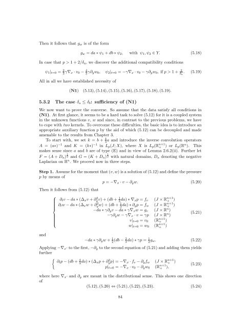
Then it follows that gw is of the form
gw = da ∗ ψ1 + db ∗ ψ2, with ψ1, ψ2 ∈ Y. (5.18)
In case that p > 1 + 2/δa, we discover the additional compatibility conditions
ψ1|t=0 = 2
3γ∇x · v0 − 4
3γ∂yw0, ψ2|t=0 = −γ∇x · v0 − γ∂yw0, if p > 1 + 2 . (5.19)
δa
All in all we have established necessity of
(N1) (5.13), (5.14), (5.15), (5.16), (5.17), (5.18), (5.19).
5.3.2 The case δa ≤ δb: sufficiency of (N1)
We now want to prove the converse. So assume that the data satisfy all conditions in
(N1). At first glance, it seems to be a hard task to solve (5.12) for it is a coupled system
in the unknown functions v, w and since, in contrast to the previous problems, we have
to cope with two kernels. To overcome these difficulties, the basic idea is to introduce an
appropriate auxiliary function p by the aid of which (5.12) can be decoupled and made
amenable to the results from Chapter 3.
a and introduce the inverse convolution operators
To start with, we set k = b + 4
3
A = (a∗) −1 and K = (k∗) −1 in Lp(J; X), where X is Lp(R n+1
+ ) or Lp(Rn ). This
makes sense since a and b are of type (E) and in view of Lemma 2.6.2(ii). Further let
F = (A + Dn) 1
2 and G = (K + Dn) 1
2 with natural domains, Dn denoting the negative
Laplacian on R n . We proceed now in three steps.
Step 1. Assume for the moment that (v, w) is a solution of (5.12) and define the pressure
p by means of
p = −∇x · v − ∂yw. (5.20)
Then it follows from (5.12) that
and
⎧
⎪⎨
⎪⎩
∂tv − da ∗ (∆xv + ∂2 yv) + (db + 1
∂tw − da ∗ (∆xw + ∂2 yw) + (db + 1
3da) ∗ ∇xp = fv (J × R n+1
+ )
3da) ∗ ∂yp = fw (J × R n+1
+ )
−da ∗ γ∂yv − da ∗ γ∇xw = gv (J × R n )
−γ∂yw − γ∇x · v = γp (J × R n )
v|t=0 = v0 (R n+1
+ )
w|t=0 = w0 (R n+1
+ )
(5.21)
−da ∗ γ∂yw + 1 2
1
2 (db − 3da) ∗ γp = 2gw. (5.22)
Applying −∇x· to the first, −∂y to the second equation of (5.21) and adding them yields
further
�
∂tp − (db + 4
3da) ∗ (∆xp + ∂2 yp) = −∇x · fv − ∂yfw (J × R n+1
+ )
p|t=0 = −∇x · v0 − ∂yw0 (R n+1
+ ),
(5.23)
where here ∇x· and ∂y are meant in the distributional sense. This shows one direction
of
(5.12), (5.20) ⇔ (5.21), (5.22), (5.23). (5.24)
84