Quasilinear parabolic problems with nonlinear boundary conditions

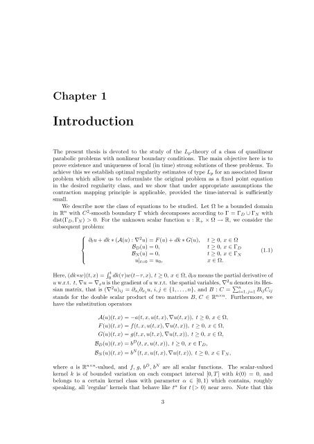
Chapter 1
Introduction
The present thesis is devoted to the study of the Lp-theory of a class of quasilinear
parabolic problems with nonlinear boundary conditions. The main objective here is to
prove existence and uniqueness of local (in time) strong solutions of these problems. To
achieve this we establish optimal regularity estimates of type Lp for an associated linear
problem which allow us to reformulate the original problem as a fixed point equation
in the desired regularity class, and we show that under appropriate assumptions the
contraction mapping principle is applicable, provided the time-interval is sufficiently
small.
We describe now the class of equations to be studied. Let Ω be a bounded domain
in R n with C 2 -smooth boundary Γ which decomposes according to Γ = ΓD ∪ ΓN with
dist(ΓD, ΓN) > 0. For the unknown scalar function u : R+ × Ω → R, we consider the
subsequent problem:
⎧
⎪⎨
⎪⎩
∂tu + dk ∗ (A(u) : ∇ 2 u) = F (u) + dk ∗ G(u), t ≥ 0, x ∈ Ω
BD(u) = 0, t ≥ 0, x ∈ ΓD
BN(u) = 0, t ≥ 0, x ∈ ΓN
u|t=0 = u0, x ∈ Ω.
(1.1)
Here, (dk∗w)(t, x) = � t
0 dk(τ)w(t−τ, x), t ≥ 0, x ∈ Ω, ∂tu means the partial derivative of
u w.r.t. t, ∇u = ∇xu is the gradient of u w.r.t. the spatial variables, ∇2u denotes its Hessian
matrix, that is (∇2u)ij = ∂xi∂xj u, i, j ∈ {1, . . . , n}, and B : C = �n i=1, j=1 BijCij
stands for the double scalar product of two matrices B, C ∈ Rn×n . Furthermore, we
have the substitution operators
A(u)(t, x) = −a(t, x, u(t, x), ∇u(t, x)), t ≥ 0, x ∈ Ω,
F (u)(t, x) = f(t, x, u(t, x), ∇u(t, x)), t ≥ 0, x ∈ Ω,
G(u)(t, x) = g(t, x, u(t, x), ∇u(t, x)), t ≥ 0, x ∈ Ω,
BD(u)(t, x) = b D (t, x, u(t, x)), t ≥ 0, x ∈ ΓD,
BN(u)(t, x) = b N (t, x, u(t, x), ∇u(t, x)), t ≥ 0, x ∈ ΓN,
where a is R n×n -valued, and f, g, b D , b N are all scalar functions. The scalar-valued
kernel k is of bounded variation on each compact interval [0, T ] with k(0) = 0, and
belongs to a certain kernel class with parameter α ∈ [0, 1) which contains, roughly
speaking, all ’regular’ kernels that behave like t α for t (> 0) near zero. Note that this
3