Quasilinear parabolic problems with nonlinear boundary conditions

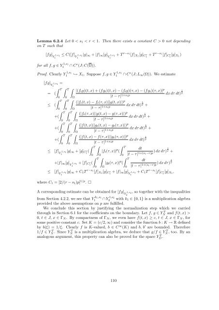
Lemma 6.2.4 Let 0 < s1 < r < 1. Then there exists a constant C > 0 not depending
on T such that
[fg] Y 1,s 1
1
for all f, g ∈ Y 1,s1
1
Proof. Clearly Y 1,s1
1
≤ C([f] 1,s
Y 1 |g|∞ + |f|∞[g] 1,s
1
Y 1 + T
1
r−s1 [f]X1 [g]C r 1 + T r−s1 [f]C r[g]X1 )
1
∩ C r (J; C(Ω)).
↩→ X1. Suppose f, g ∈ Y 1,s1
1
∩ C r (J; L∞(Ω)). We estimate
[fg] 1,s
Y 1 =
1
� T � T �
|(ftg)(t, x) + (fgt)(t, x) − (ftg)(τ, x) − (fgt)(τ, x)|
= (
0 0 Ω
p
|t − τ| 1+s1p
dx dτ dt) 1
p
� T � T �
(|ft(t, x) − ft(τ, x)||g(t, x)|)
≤ (
0 0 Ω
p
|t − τ| 1+s1p dx dτ dt) 1
p +
� T � T �
(|ft(τ, x)||g(t, x) − g(τ, x)|)
+(
0 0 Ω
p
|t − τ| 1+s1p dx dτ dt) 1
p +
� T � T �
(|f(t, x)||gt(t, x) − gt(τ, x)|)
+(
0 0 Ω
p
|t − τ| 1+s1p dx dτ dt) 1
p +
� T � T �
(|f(t, x) − f(τ, x)||gt(τ, x)|)
+(
0 0 Ω
p
|t − τ| 1+s1p dx dτ dt) 1
p
≤ [f] 1,s
Y 1 |g|∞ + [g]C
1
r 1 (
� T �
|ft(τ, x)|
0 Ω
p � T dt
(
) dx dτ)1 p +
0 |t − τ| 1+(s1−r)p
+|f|∞[g] 1,s
Y 1 + [f]C
1
r 1 (
� T �
|gt(τ, x)|
0 Ω
p � T dt
(
) dx dτ)1 p
0 |t − τ| 1+(s1−r)p
≤ [f] 1,s
Y 1 |g|∞ + C1T
1
r−s1 [f]X1 [g]C r 1 + |f|∞[g] 1,s
Y 1 + C1T
1
r−s1 [f]C r[g]X1 ,
1
where C1 = [2/(r − s1)p] 1/p . �
A corresponding estimate can be obtained for [fg] 1,s
Y 2 , so together with the inequalities
2
from Section 4.2.2, we see that Y k1,s1
1 ∩ Y 1,s2
2 with k1 ∈ {0, 1} is a multiplication algebra
provided the above assumptions on p are fulfilled.
We conclude this section by justifying the normalization step which we carried
through in Section 6.1 for the coefficients on the boundary. Let f, g ∈ Y T N and f(t, x) >
0, t ∈ J, x ∈ ΓN. By compactness of ΓN, we even have f(t, x) ≥ c, t ∈ J, x ∈ ΓN, for
some positive constant c. Set K = (c/2, ∞) and consider the function b : K → R defined
by b(ξ) = 1/ξ. Clearly f is K-valued, b ∈ C ∞ (K) and b, b ′ are bounded. Therefore
1/f ∈ Y T N . Since Y T N is a multiplication algebra, we deduce that g/f ∈ Y T N , too. By an
analogous argument, this property can also be proved for the space Y T D .
110