Quasilinear parabolic problems with nonlinear boundary conditions

More documents

Recommendations

Info

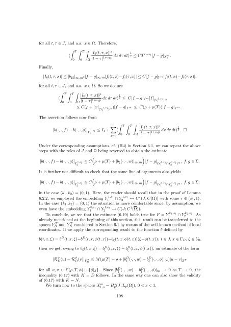
for all t, τ ∈ J, and a.a. x ∈ Ω. Therefore, Finally, � T � T � ( 0 0 Ω |I5(t, τ, x)| p 1 dx dτ dt) p ≤ CT |t − τ| 1+s1p r−s1 [f − g]X m 1 . |I6(t, τ, x)| ≤ |bξξ| ∞, m 2|f − g|∞, m|ft(t, x)−ft(τ, x)| ≤ C[f − g]Y m|ft(t, x)−ft(τ, x)|. for all t, τ ∈ J, and a.a. x ∈ Ω. So we deduce � T � T � ( 0 0 The assertion follows now from Ω [b(·, ·, f) − b(·, ·, g)] Y 1,s 1 1 |I6(t, τ, x)| p 1 dx dτ dt) |t − τ| 1+s1p p ≤ C|f − g|Y m[f] (Y 1,s1 1 ) m ≤ C(ρ + [w] 1,s (Y 1 1 ) m)|f − g|Y m ≤ C(ρ + µ(T ))|f − g|Y m. ≤ I1 + 6� ( j=3 � T � T 0 0 � Ω |Ij(t, τ, x)| p 1 dx dτ dt) p . � |t − τ| 1+s1p Under the corresponding assumptions, cf. (H4) in Section 6.1, we can repeat the above steps with the roles of J and Ω being reversed to obtain the estimate � � ≤ C ρ + µ(T ) + |bξ(·, ·, w)|∞, m [b(·, ·, f) − b(·, ·, g)] Y 1,s 2 2 |f − g| (Y 1,s 1 1 It is further not difficult to check that the same line of arguments also yields � � ≤ C ρ + µ(T ) + |bξ(·, ·, w)|∞, m [b(·, ·, f) − b(·, ·, g)] Y 1,s 2 2 |f − g| (Y 0,s 1 1 ∩Y 1,s2 2 ) m, f, g ∈ Σ. ∩Y 1,s2 2 ) m, f, g ∈ Σ, in the case (k1, k2) = (0, 1). Here, the reader should recall that in the proof of Lemma 6.2.2, we employed the embedding Y 1,s1 1 ∩ Y 1,s2 2 ↩→ Cr (J; C( ¯ Ω)) with some r ∈ (s1, 1). In the case (k1, k2) = (0, 1) the situation is more comfortable since, by assumption, we even have the embedding Y 0,s1 1 ∩ Y 1,s2 2 ↩→ C(J; C1 (Ω)). To conclude, we see that the estimate (6.19) holds true for F = Y k1,s1 1 ∩ Y k2,s2 2 . As already mentioned at the beginning of this section, this result can be transferred to the spaces Y T D and Y T N considered in Section 6.1 by means of the well-known method of local coordinates. If we apply the corresponding result to the function b defined by b(t, x, ξ) = b D (t, x, ξ)−b D (t, x, φ(t, x))−bξ(t, x, φ(t, x))(ξ−φ(t, x)), t ∈ J, x ∈ ΓD, ξ ∈ U0, then we get, owing to bξ(t, x, ξ) = bD ξ (t, x, ξ) − bD ξ (t, x, φ(t, x)), an estimate of the form |R φ D (u) − Rφ D (v)| Y T D ≤ M(µ(T ) + ρ + |bDξ (·, ·, w) − bDξ (·, ·, φ)|∞)|u − v| ZT for all u, v ∈ Σ(ρ, T, φ) ∪ {φ|J}. Since |b D ξ (·, ·, w) − bD ξ (·, ·, φ)|∞ → 0 as T → 0, the inequality (6.17) with K = D follows. In the same way one can also show the validity of (6.17) with K = N. We turn now to the spaces X m 1, s = Hs p(J; Lp(Ω)), 0 < s < 1. 108
Lemma 6.2.3 Let 0 < s < s0 < 1, ρ ∈ (0, ρ0], and w ∈ Xm 1, s0 ∩ C(J; C(Ω)) be a fixed K-valued function. Let further Σ ′ be as described above. Suppose that b is as in Lemma 6.2.1 with r ∈ (s, 1) and bξ ∈ L∞(J × Ω × K, Rm ). Then there exists a constant C > 0 not depending on T and ρ such that [b(·, ·, f) − b(·, ·, g)]X1, s ≤ Cµ(T )(|f − g|X m 1, s 0 Proof. Let f, g be arbitrary functions in Σ ′ . Put + |f − g|∞, m), f, g ∈ Σ ′ . ω(t, h, x) = b(t + h, x, f(t + h, x))−b(t + h, x, g(t + h, x))−b(t, x, f(t, x))+b(t, x, g(t, x)) for t, t + h ∈ J, and x ∈ Ω. Then [b(·, ·, f)−b(·, ·, g)]X1, s � = ( Ω � T 0 ( � 1 0 σ −2s � 1 ( |V (t, σ)| V (t, σ) Similarly as in the proof of Lemma 6.2.1 we may establish 2 dσ |ω(t, h, x)| dh) σ |ω(t, h, x)| ≤ |bξ|∞, m |f(t + h, x) − f(t, x) − g(t + h, x) + g(t, x)| + ) p 2 dt dx) 1 p . + CHL|f − g|∞, m(|f(t + h, x) − f(t, x)| + |g(t + h, x) − g(t, x)| + Cb(x)|h| r ) for all t, t + h ∈ J and a.a. x ∈ Ω. With Θ := ( we thus obtain ≤ ( � T ( � 1 0 0 � T � 1 [b(·,·, f) − b(·, ·, g)]X1, s ≤ � ≤ C � ≤ C � ≤ Cµ(T ) 0 ( 0 σ −2s � 1 ( |V (t, σ)| σ −2s � 1 ( |V (t, σ)| V (t, σ) V (t, σ) |h| r 2 dσ dh) σ σ r 2 dσ dh) σ ) p 2 dt) 1 p ) p 2 dt) 1 p = T 1 p √ 2(r−s) , [f − g]X m 1, s + |f − g|∞, m([f]X m 1, s + [g]X m 1, s + |Cb| Lp(Ω)Θ) [f − g]X m 1, s + |f − g|∞([f − w]X m 1, s + [g − w]X m 1, s + [w]X m 1, s [f − g]X m + |f − g|∞, 1, s m([f − w]X 0 m + [g − w]X 1, s0 m 1, s0 ≤ Cµ(T )([f − g]X m 1, s 0 + |f − g|∞, m). � � � + µ(T )) � + 1) Lemma 6.2.3 and the trivial inequality |Bf −Bg|X ≤ Cµ(T )|f −g|∞, m yield the estimate (6.20), which we were aiming at. This completes the proof of the inequality (6.16), since we have ZT ∇ ↩→ H(1+α)/2 p (J; Lp(Ω)) ∩ C(J × Ω) and (1 + α)/2 > α. We conclude this paragraph with a result on pointwise multiplication which have been used several times in the previous sections. In Section 4.2.2 we have already seen that the space Y 0,s1 1 ∩ Y 0,s2 2 forms a multiplication algebra if the embedding Y 0,s1 1 ∩ Y 0,s2 2 ↩→ C(J; C(Ω)) is valid. We will show under the above assumptions on p that this is true also for Y k1,s1 1 ∩ Y 1,s2 2 with k1 = 0, 1. As before, we shall only consider the seminorm terms of highest order. 109
Page 1 and 2:
Gutachter: Quasilinear parabolic pr
Page 3 and 4:
Contents 1 Introduction 3 2 Prelimi
Page 5 and 6:
Chapter 1 Introduction The present
Page 7 and 8:
to assume that m, c are bounded fun
Page 9 and 10:
We give now an overview of the cont
Page 11 and 12:
conditions of order ≤ 1. Sections
Page 13 and 14:
Chapter 2 Preliminaries 2.1 Some no
Page 15 and 16:
Clearly, φA ∈ [0, π) and φA
Page 17 and 18:
Definition 2.2.3 Let X and Y be Ban
Page 19 and 20:
µ ∈ Σφα }. Let N ∈ N, Tj
Page 21 and 22:
We remark that a theorem of the Dor
Page 23 and 24:
Here f(A, ·) ∈ H0(Σ π 2 +η; B
Page 25 and 26:
Further, K ∞ (α, θa) := {a ∈
Page 27 and 28:
Using (2.19) for aω and bω yields
Page 29 and 30:
2.7 Evolutionary integral equations
Page 31 and 32:
Example 2.8.1 For J = [0, T ] and a
Page 33:
We conclude this section by illustr
Page 36 and 37:
kernel a. The operator B is inverti
Page 38 and 39:
x := f(0) ∈ X exists and we are l
Page 40 and 41:
with two positive constants C1, C2
Page 42 and 43:
with two positive constants C1 and
Page 44 and 45:
derivative theorem to this pair of
Page 46 and 47:
3.2 A general trace theorem Let X b
Page 48 and 49:
3.3 More time regularity for Volter
Page 50 and 51:
Theorem 3.4.2 Suppose X is a Banach
Page 52 and 53:
Our next objective is to show neces
Page 54 and 55:
Let u1 be the restriction of v1 to
Page 56 and 57:
Proof. We begin with the necessity
Page 59 and 60: Chapter 4 Linear Problems of Second
Page 61 and 62: The strategy for solving (4.1) is n
Page 63 and 64: Since ψj ≡ 1 on supp ϕj, we may
Page 65 and 66: Turning to (c), let g ∈ Ξi+1 and
Page 67 and 68: endowed with the norm | · | Y T 2
Page 69 and 70: We remark that the constant C2 stem
Page 71 and 72: One can then construct functions a
Page 73 and 74: analogous to (4.17), shows that S i
Page 75 and 76: Apply now V#, i+1 := I + k ∗ A#(
Page 77 and 78: Given a function v ∈ H 2 p(R n+1
Page 79 and 80: v is a solution of (4.40) on Ji+1 :
Page 81 and 82: Chapter 5 Linear Viscoelasticity In
Page 83 and 84: where δij denotes Kronecker’s sy
Page 85 and 86: problem ⎧ ⎪⎨ ⎪⎩ ∂tv −
Page 87 and 88: To see the converse direction, supp
Page 89 and 90: and up solves � Aup − ∆xup
Page 91 and 92: It can be written as where l(z, ξ)
Page 93 and 94: elongs to H∞ (Σ π 2 +η × Ση
Page 95 and 96: which allows us to write the first
Page 97 and 98: Chapter 6 Nonlinear Problems 6.1 Qu
Page 99 and 100: sufficiently small, say T ≤ T1
Page 101 and 102: (d) bD ∈ C(J0 × ΓD × U0), ∃C
Page 103 and 104: which entails (6.14). Corresponding
Page 105 and 106: substitution operators to be studie
Page 107 and 108: for all t, τ ∈ J, ξ, η ∈ K,
Page 109: to write where h2(t, τ, x) = h21(t
Page 113 and 114: Bibliography [1] Albrecht, D.: Func
Page 115 and 116: [54] Lunardi, A.: On the heat equat
Page 117 and 118: kleines T mit Hilfe des Kontraktion
Page 119: Personal Details Curriculum Vitae N
show all

Quasilinear parabolic problems with nonlinear boundary conditions

Create successful ePaper yourself

Delete template?

Save as template?