Quasilinear parabolic problems with nonlinear boundary conditions

More documents

Recommendations

Info

Strict contractivity of Υ can be established in similar fashion. Let u, ū ∈ Σ(ρ, T, φ) and put v = Υ(u) and ¯v = Υ(ū). Then ¯v − v satisfies ⎧ ∂t(¯v − v) + dk ∗ A0 : ∇ ⎪⎨ ⎪⎩ 2 (¯v − v) = F (ū) − F (u) + dk ∗ (G(ū) − G(u)) (J × Ω) +dk ∗ (((A0−A(ū)):∇ 2ū)−(A0−A(u)):∇ 2u) B◦ D (φ)(¯v − v) = −(Rφ D (ū) − Rφ D (u)) (J × ΓD) B◦ N (φ)(¯v − v) = −(Rφ N (ū) − Rφ N (u)) (J × ΓN) (¯v − v)|t=0 = 0 (Ω), whence |¯v − v| Z T ≤ M1 � |G(ū) − G(u) + (((A0−A(ū)):∇ 2 ū)−(A0−A(u)):∇ 2 u)| XT + |F (ū) − F (u)| XT + |R 1 φ D (ū) − Rφ D (u)| Y T D ≤ M(µ(T ) + ρ)|ū − u| Z T , + |Rφ N (ū) − Rφ N (u)| Y T N by maximal regularity and the estimates from Theorem 6.1.1. Here the constants M and µ(T ) are like those in (6.18). Hence Υ becomes a strict contraction, when ρ and T are selected sufficiently small. The assertion follows now by the contraction mapping principle and the fact that fixed points of Υ correspond to solutions of (6.1) for small time-intervals J = [0, T ]. � Remarks 6.1.1 (i) The statement of Theorem 6.1.2 is also true, if k is of the form k = k1 + dl ∗ k1, where k1 is like k in (H1) and l ∈ BVloc(R+) with l(0) = l(0+) = 0. (ii) One can further replace k on the right-hand side of (6.1) by an arbitrary kernel k1 ∈ BVloc(R+) ∩ K 1 (1 + α1, θ1) with k(0) = 0, α1 ≥ α, θ1 < π, and the theorem still holds true. 6.2 Nemytskij operators for various function spaces This paragraph can be regarded as an appendix to Section 6.1. Its purpose is to complete the proof of Theorem 6.1.1. We still have to show certain mapping properties and Lipschitz estimates for the substitution operators which involve the nonlinear functions f, b D and b N , cf. the beginning of Section 6.1. The Nemytskij operators under consideration act on the function spaces which arose as natural regularity classes for the inhomogeneities in the treatment of the linear problem (6.8), and turned out to be the spaces XT 1 , Y T D , and Y T N , see (6.2), (6.3), (6.4) for their definitions. These are anisotropic Bessel-potential and Sobolev-Slobodeckij spaces in domains, respectively, compact manifolds in the euclidean space, which means that the subject of this section is not altogether trivial. We remark that in order to get the desired estimates for Y T D and Y T N , which are spaces on J × ΓD resp. J × ΓN, one considers first the corresponding spaces in domains (w.r.t. the spatial variable). The results obtained for the latter can then be transferred to Y T D and Y T N by means of the standard method of local coordinates. In what is to follow, we shall focus on the first step. As to the second step, we merely point out that the fact that Ω (in Section 6.1) has a (compact) C2 boundary ensures that the smoothness of bD resp. bN w.r.t. the spatial variable x is preserved under the local coordinate transformations studied in Section 4.3, which flatten the boundary. The reader is further reminded of the embedding ZT ↩→ C(J; C1 (Ω)), which is valid in view of the assumption (H2), and which considerably simplifies the investigation of the 102 �
substitution operators to be studied in this section. Note that thanks to this embedding, we do not require any growth conditions on the nonlinearities. It should also be remarked that all nonlinearities appearing in the subsequent estimates are tacitly assumed to be Carathéodory functions so that we do not have to be concerned with measurability questions, cf. Appell and Zabrejko [4, Section 1.4]. Notice that this corresponds to the regularity assumptions in (H4). We fix now the notation used in this section. Let J = [0, T ] (0 < T ≤ T0), and Ω be a bounded domain in R n with C 1 boundary. For p ∈ (1, ∞) and m ∈ N we introduce the symbols X m := Lp(J × Ω, R m ), X m 1 := H 1 p(J; Lp(Ω, R m )), and X m 2 := Lp(J; H 1 p(Ω, R m )). Our interest lies in the spaces X m 1, s := Hs p(J; Lp(Ω, R m )), (Y k,s 1 ) m := B k+s pp (J; Lp(Ω, R m )), (Y k,s 2 ) m := Lp(J; B k+s pp (Ω, R m )), where k ∈ {0, 1} and s ∈ (0, 1). But we will also deal with the space (C r 1 )m := C r (J; C(Ω, R m )), where r ∈ [0, 1). For more brevity, we omit the parameter m in all these notations if m = 1, i.e. we write X = X 1 , Xi = X 1 i and so forth. 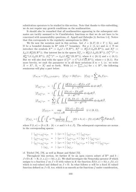With |z| := � m i=1 |zi| for z ∈ R m , the following seminorms will play a part below: [f]X m 1, s |f|∞, m = |f| L∞(J×Ω,R m ), [f]X m 1 = |∂tf|X m, [f]X m 2 = [f] k,s (Y1 ) m � T � T � = ( 0 0 Ω [f] 0,s (Y2 ) m � T � � [f] 1,s (Y2 ) = ( 0 Ω Ω m = n� � T � ( i=1 0 Ω Ω � = ( Ω |∂ k t f(t, x) − ∂ k t f(τ, x)| p |t − τ| 1+sp |f(t, x) − f(t, y)| p |x − y| n+sp � |f(t, x) − f(τ, x)| [f] (Cr 1 ) m = sup t�=τ∈J, x∈Ω |t − τ| r � 1 � � T 0 ( 0 σ −2s 1 ( |V (t, σ)| n� i=1 dx dy dt) 1 p , dx dτ dt) 1 p , |∂xif|X m, |∂xif(t, x) − ∂xif(t, y)|p |x − y| n+sp dx dy dt) 1 p , V (t, σ) (r ∈ (0, 1)), 2 dσ |f(t + h, x) − f(t, x)| dh) σ ) p 2 dt dx) 1 p , where V (t, σ) = {h ∈ R : |h| < σ and t+h ∈ J}. The subsequent expressions are norms in the corresponding spaces: | · | 0,s (Y 1 1 ∩Y 0,s2 2 ) m = | · |Xm + [ · ] (Y 0,s1 1 ) m + [ · ] 0,s (Y 2 2 ) m, | · | 0,s (Y 1 1 ∩Y 1,s2 2 ) m = | · |Xm + [ · ] (Y 0,s1 1 ) m + [ · ]Xm 2 + [ · ] (Y 1,s2 2 ) m, | · | 1,s (Y 1 1 ∩Y 1,s2 2 ) m = | · |Xm + [ · ]Xm 1 + [ · ] (Y 1,s1 1 ) m + [ · ]Xm 2 + [ · ] (Y 1,s2 2 ) m, | · |Xm 1, s = | · |Xm + [ · ]Xm 1, s , cf. Triebel [78], [79], as well as Runst and Sickel [72]. Throughout this section, let further K be an open convex subset of R m and b : J ×Ω×K → R, (t, x, ξ) ↦→ b(t, x, ξ). We shall investigate the Nemytskij operator B which assigns to a function f on J × Ω with values in K the function Bf(t, x) = b(t, x, f(t, x)) which is real-valued and defined on J × Ω. In what follows w will be a fixed K-valued function defined on J ×Ω, too, which is as smooth as the functions f under consideration, 103
Page 1 and 2:
Gutachter: Quasilinear parabolic pr
Page 3 and 4:
Contents 1 Introduction 3 2 Prelimi
Page 5 and 6:
Chapter 1 Introduction The present
Page 7 and 8:
to assume that m, c are bounded fun
Page 9 and 10:
We give now an overview of the cont
Page 11 and 12:
conditions of order ≤ 1. Sections
Page 13 and 14:
Chapter 2 Preliminaries 2.1 Some no
Page 15 and 16:
Clearly, φA ∈ [0, π) and φA
Page 17 and 18:
Definition 2.2.3 Let X and Y be Ban
Page 19 and 20:
µ ∈ Σφα }. Let N ∈ N, Tj
Page 21 and 22:
We remark that a theorem of the Dor
Page 23 and 24:
Here f(A, ·) ∈ H0(Σ π 2 +η; B
Page 25 and 26:
Further, K ∞ (α, θa) := {a ∈
Page 27 and 28:
Using (2.19) for aω and bω yields
Page 29 and 30:
2.7 Evolutionary integral equations
Page 31 and 32:
Example 2.8.1 For J = [0, T ] and a
Page 33:
We conclude this section by illustr
Page 36 and 37:
kernel a. The operator B is inverti
Page 38 and 39:
x := f(0) ∈ X exists and we are l
Page 40 and 41:
with two positive constants C1, C2
Page 42 and 43:
with two positive constants C1 and
Page 44 and 45:
derivative theorem to this pair of
Page 46 and 47:
3.2 A general trace theorem Let X b
Page 48 and 49:
3.3 More time regularity for Volter
Page 50 and 51:
Theorem 3.4.2 Suppose X is a Banach
Page 52 and 53:
Our next objective is to show neces
Page 54 and 55: Let u1 be the restriction of v1 to
Page 56 and 57: Proof. We begin with the necessity
Page 59 and 60: Chapter 4 Linear Problems of Second
Page 61 and 62: The strategy for solving (4.1) is n
Page 63 and 64: Since ψj ≡ 1 on supp ϕj, we may
Page 65 and 66: Turning to (c), let g ∈ Ξi+1 and
Page 67 and 68: endowed with the norm | · | Y T 2
Page 69 and 70: We remark that the constant C2 stem
Page 71 and 72: One can then construct functions a
Page 73 and 74: analogous to (4.17), shows that S i
Page 75 and 76: Apply now V#, i+1 := I + k ∗ A#(
Page 77 and 78: Given a function v ∈ H 2 p(R n+1
Page 79 and 80: v is a solution of (4.40) on Ji+1 :
Page 81 and 82: Chapter 5 Linear Viscoelasticity In
Page 83 and 84: where δij denotes Kronecker’s sy
Page 85 and 86: problem ⎧ ⎪⎨ ⎪⎩ ∂tv −
Page 87 and 88: To see the converse direction, supp
Page 89 and 90: and up solves � Aup − ∆xup
Page 91 and 92: It can be written as where l(z, ξ)
Page 93 and 94: elongs to H∞ (Σ π 2 +η × Ση
Page 95 and 96: which allows us to write the first
Page 97 and 98: Chapter 6 Nonlinear Problems 6.1 Qu
Page 99 and 100: sufficiently small, say T ≤ T1
Page 101 and 102: (d) bD ∈ C(J0 × ΓD × U0), ∃C
Page 103: which entails (6.14). Corresponding
Page 107 and 108: for all t, τ ∈ J, ξ, η ∈ K,
Page 109 and 110: to write where h2(t, τ, x) = h21(t
Page 111 and 112: Lemma 6.2.3 Let 0 < s < s0 < 1, ρ
Page 113 and 114: Bibliography [1] Albrecht, D.: Func
Page 115 and 116: [54] Lunardi, A.: On the heat equat
Page 117 and 118: kleines T mit Hilfe des Kontraktion
Page 119: Personal Details Curriculum Vitae N
show all

Quasilinear parabolic problems with nonlinear boundary conditions

Create successful ePaper yourself

Delete template?

Save as template?