Quasilinear parabolic problems with nonlinear boundary conditions
Quasilinear parabolic problems with nonlinear boundary conditions Quasilinear parabolic problems with nonlinear boundary conditions
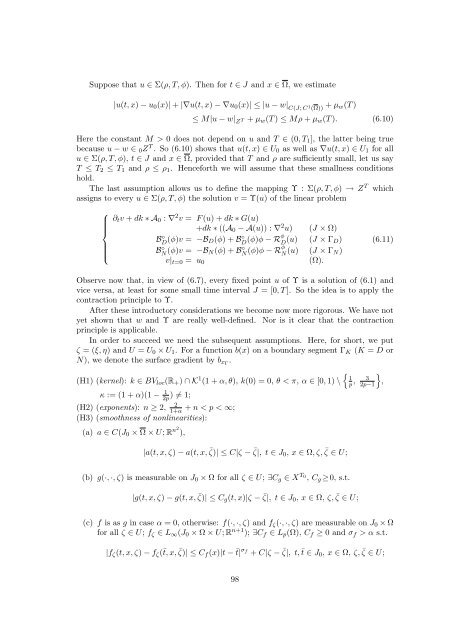
Suppose that u ∈ Σ(ρ, T, φ). Then for t ∈ J and x ∈ Ω, we estimate |u(t, x) − u0(x)| + |∇u(t, x) − ∇u0(x)| ≤ |u − w| C(J; C 1 (Ω)) + µw(T ) ≤ M|u − w| Z T + µw(T ) ≤ Mρ + µw(T ). (6.10) Here the constant M > 0 does not depend on u and T ∈ (0, T1], the latter being true because u − w ∈ 0Z T . So (6.10) shows that u(t, x) ∈ U0 as well as ∇u(t, x) ∈ U1 for all u ∈ Σ(ρ, T, φ), t ∈ J and x ∈ Ω, provided that T and ρ are sufficiently small, let us say T ≤ T2 ≤ T1 and ρ ≤ ρ1. Henceforth we will assume that these smallness conditions hold. The last assumption allows us to define the mapping Υ : Σ(ρ, T, φ) → Z T which assigns to every u ∈ Σ(ρ, T, φ) the solution v = Υ(u) of the linear problem ⎧ ⎪⎨ ⎪⎩ ∂tv + dk ∗ A0 : ∇2v = F (u) + dk ∗ G(u) +dk ∗ ((A0 − A(u)) : ∇2u) (J × Ω) B◦ D (φ)v = −BD(φ) + B◦ D (φ)φ − Rφ D (u) B (J × ΓD) ◦ N (φ)v = −BN(φ) + B◦ N (φ)φ − Rφ N (u) (J × ΓN) (Ω). v|t=0 = u0 (6.11) Observe now that, in view of (6.7), every fixed point u of Υ is a solution of (6.1) and vice versa, at least for some small time interval J = [0, T ]. So the idea is to apply the contraction principle to Υ. After these introductory considerations we become now more rigorous. We have not yet shown that w and Υ are really well-defined. Nor is it clear that the contraction principle is applicable. In order to succeed we need the subsequent assumptions. Here, for short, we put ζ = (ξ, η) and U = U0 × U1. For a function b(x) on a boundary segment ΓK (K = D or N), we denote the surface gradient by bxΓ . (H1) (kernel): k ∈ BVloc(R+) ∩ K1 � 1 (1 + α, θ), k(0) = 0, θ < π, α ∈ [0, 1) \ p , � 3 2p−1 , κ := (1 + α)(1 − 1 2p ) �= 1; 2 (H2) (exponents): n ≥ 2, 1+α + n < p < ∞; (H3) (smoothness of nonlinearities): (a) a ∈ C(J0 × Ω × U; Rn2), |a(t, x, ζ) − a(t, x, ¯ ζ)| ≤ C|ζ − ¯ ζ|, t ∈ J0, x ∈ Ω, ζ, ¯ ζ ∈ U; (b) g(·, ·, ζ) is measurable on J0 × Ω for all ζ ∈ U; ∃Cg ∈ X T0 , Cg ≥0, s.t. |g(t, x, ζ) − g(t, x, ¯ ζ)| ≤ Cg(t, x)|ζ − ¯ ζ|, t ∈ J0, x ∈ Ω, ζ, ¯ ζ ∈ U; (c) f is as g in case α = 0, otherwise: f(·, ·, ζ) and fζ(·, ·, ζ) are measurable on J0 × Ω for all ζ ∈ U; fζ ∈ L∞(J0 × Ω × U; R n+1 ); ∃Cf ∈ Lp(Ω), Cf ≥ 0 and σf > α s.t. |fζ(t, x, ζ) − fζ(¯t, x, ¯ ζ)| ≤ Cf (x)|t − ¯t| σf + C|ζ − ¯ ζ|, t, ¯t ∈ J0, x ∈ Ω, ζ, ¯ ζ ∈ U; 98
(d) bD ∈ C(J0 × ΓD × U0), ∃Cb1 ∈ Lp(ΓD), Cb1 ≥ 0, ∃Cb2 ∈ Lp(J), Cb2 ≥ 0, and ∃σ2 > 1 − 1 p such that in case κ < 1: ∃σ1 > κ s.t. |b D xΓ (t, x, ξ) − bD xΓ (t, ¯x, ξ)| ≤ Cb2 (t)|x − ¯x|σ2 , (6.12) |b D ξ (t, x, ξ) − bD ξ (¯t, x, ξ)| ≤ Cb1 (x)|t − ¯t| σ1 , |b D xΓξ (t, x, ξ) − bD xΓξ (t, ¯x, ¯ ξ)| ≤ Cb2 (t)|x − ¯x|σ2 + C|ξ − ¯ ξ|, (6.13) |b D ξξ (t, x, ξ) − bD ξξ (t, ¯x, ¯ ξ)| ≤ C(|x − ¯x| σ2 + |ξ − ¯ ξ|), and in case κ > 1: ∃σ1 > κ − 1 s.t. (6.12), (6.13), |b D t (t, x, ξ) − b D t (¯t, x, ξ)| ≤ Cb1 (x)|t − ¯t| σ1 , |b D tξ (t, x, ξ) − bD tξ (¯t, x, ¯ ξ)| ≤ Cb1 (x)|t − ¯t| σ1 + C|ξ − ¯ ξ|, |b D ξξ (t, x, ξ) − bD ξξ (¯t, ¯x, ¯ ξ)| ≤ C(|t − ¯t| σ1 + |x − ¯x| σ2 + |ξ − ¯ ξ|), all these inequalities being true for t, ¯t ∈ J0, x, ¯x ∈ ΓD, ξ, ¯ ξ ∈ U0; each of the derivatives of b D occurring above is Carathéodory and essentially bounded on J0 × ΓD × U0; (e) bN ∈ C(J0×ΓN ×U), bN ζ ∈ L∞(J0×ΓN ×U; Rn+1 ) is Carathéodory, ∃Cb1 ∈ Lp(ΓN), , s.t. Cb1 ≥ 0, ∃Cb2 ∈ Lp(J), Cb2 ≥ 0, ∃σ1 > (1 + α)( 1 1 2 − 2p ), ∃σ2 > 1 − 1 p |b N (t, x, ζ) − b N (¯t, ¯x, ζ)| ≤ Cb1 (x)|t − ¯t| σ1 + Cb2 (t)|x − ¯x|σ2 , |b N ζ (t, x, ζ) − bN ζ (¯t, ¯x, ¯ ζ)| ≤ Cb1 (x)|t − ¯t| σ1 + Cb2 (t)|x − ¯x|σ2 + C|ζ − ¯ ζ|, t, ¯t ∈ J0, x, ¯x ∈ ΓN, ζ, ¯ ζ ∈ U; (H4) (initial data): u0 ∈ Y0; u1 ∈ Y1, if α > 1 p (u1(x) := f(0, x, u0(x), ∇u0(x)), x ∈ Ω); f(·, ·, u0(·), ∇u0(·)), g(·, ·, u0(·), ∇u0(·)) ∈ X T0 . (H5) (compatibility): (u0(x), ∇u0(x)) ∈ U0 × U1, x ∈ Ω; b D (0, x, u0(x)) = 0, x ∈ ΓD; b N (0, x, u0(x), ∇u0(x)) = 0, x ∈ ΓN; b D t (0, x, u0(x)) + b D ξ (0, x, u0(x))u1(x) = 0, x ∈ ΓD, if α > 3 2p−1 ; (H6) (ellipticity): a(0, x, u0(x), ∇u0(x)) ∈ Sym{n}, x ∈ Ω; ∃c0 > 0 s.t. (H7) (normality): We have now the following result. a(0, x, u0(x), ∇u0(x))ϱ · ϱ ≥ c0|ϱ| 2 , x ∈ Ω, ϱ ∈ R n ; b D ξ (0, x, u0(x)) �= 0, x ∈ ΓD; b N η (0, x, u0(x), ∇u0(x)) · ν(x) �= 0, x ∈ ΓN. Theorem 6.1.1 Suppose that the assumptions (H1)-(H7) are satisfied. Let φ ∈ Z T0 be as above, and assume that ρ ≤ ρ1. Then there exists T3 ∈ (0, T2] such that for each T ∈ (0, T3] the following statements hold: 99
- Page 50 and 51: Theorem 3.4.2 Suppose X is a Banach
- Page 52 and 53: Our next objective is to show neces
- Page 54 and 55: Let u1 be the restriction of v1 to
- Page 56 and 57: Proof. We begin with the necessity
- Page 59 and 60: Chapter 4 Linear Problems of Second
- Page 61 and 62: The strategy for solving (4.1) is n
- Page 63 and 64: Since ψj ≡ 1 on supp ϕj, we may
- Page 65 and 66: Turning to (c), let g ∈ Ξi+1 and
- Page 67 and 68: endowed with the norm | · | Y T 2
- Page 69 and 70: We remark that the constant C2 stem
- Page 71 and 72: One can then construct functions a
- Page 73 and 74: analogous to (4.17), shows that S i
- Page 75 and 76: Apply now V#, i+1 := I + k ∗ A#(
- Page 77 and 78: Given a function v ∈ H 2 p(R n+1
- Page 79 and 80: v is a solution of (4.40) on Ji+1 :
- Page 81 and 82: Chapter 5 Linear Viscoelasticity In
- Page 83 and 84: where δij denotes Kronecker’s sy
- Page 85 and 86: problem ⎧ ⎪⎨ ⎪⎩ ∂tv −
- Page 87 and 88: To see the converse direction, supp
- Page 89 and 90: and up solves � Aup − ∆xup
- Page 91 and 92: It can be written as where l(z, ξ)
- Page 93 and 94: elongs to H∞ (Σ π 2 +η × Ση
- Page 95 and 96: which allows us to write the first
- Page 97 and 98: Chapter 6 Nonlinear Problems 6.1 Qu
- Page 99: sufficiently small, say T ≤ T1
- Page 103 and 104: which entails (6.14). Corresponding
- Page 105 and 106: substitution operators to be studie
- Page 107 and 108: for all t, τ ∈ J, ξ, η ∈ K,
- Page 109 and 110: to write where h2(t, τ, x) = h21(t
- Page 111 and 112: Lemma 6.2.3 Let 0 < s < s0 < 1, ρ
- Page 113 and 114: Bibliography [1] Albrecht, D.: Func
- Page 115 and 116: [54] Lunardi, A.: On the heat equat
- Page 117 and 118: kleines T mit Hilfe des Kontraktion
- Page 119: Personal Details Curriculum Vitae N
Suppose that u ∈ Σ(ρ, T, φ). Then for t ∈ J and x ∈ Ω, we estimate<br />
|u(t, x) − u0(x)| + |∇u(t, x) − ∇u0(x)| ≤ |u − w| C(J; C 1 (Ω)) + µw(T )<br />
≤ M|u − w| Z T + µw(T ) ≤ Mρ + µw(T ). (6.10)<br />
Here the constant M > 0 does not depend on u and T ∈ (0, T1], the latter being true<br />
because u − w ∈ 0Z T . So (6.10) shows that u(t, x) ∈ U0 as well as ∇u(t, x) ∈ U1 for all<br />
u ∈ Σ(ρ, T, φ), t ∈ J and x ∈ Ω, provided that T and ρ are sufficiently small, let us say<br />
T ≤ T2 ≤ T1 and ρ ≤ ρ1. Henceforth we will assume that these smallness <strong>conditions</strong><br />
hold.<br />
The last assumption allows us to define the mapping Υ : Σ(ρ, T, φ) → Z T which<br />
assigns to every u ∈ Σ(ρ, T, φ) the solution v = Υ(u) of the linear problem<br />
⎧<br />
⎪⎨<br />
⎪⎩<br />
∂tv + dk ∗ A0 : ∇2v = F (u) + dk ∗ G(u)<br />
+dk ∗ ((A0 − A(u)) : ∇2u) (J × Ω)<br />
B◦ D (φ)v = −BD(φ) + B◦ D (φ)φ − Rφ<br />
D (u)<br />
B<br />
(J × ΓD)<br />
◦ N (φ)v = −BN(φ) + B◦ N (φ)φ − Rφ<br />
N (u) (J × ΓN)<br />
(Ω).<br />
v|t=0 = u0<br />
(6.11)<br />
Observe now that, in view of (6.7), every fixed point u of Υ is a solution of (6.1) and<br />
vice versa, at least for some small time interval J = [0, T ]. So the idea is to apply the<br />
contraction principle to Υ.<br />
After these introductory considerations we become now more rigorous. We have not<br />
yet shown that w and Υ are really well-defined. Nor is it clear that the contraction<br />
principle is applicable.<br />
In order to succeed we need the subsequent assumptions. Here, for short, we put<br />
ζ = (ξ, η) and U = U0 × U1. For a function b(x) on a <strong>boundary</strong> segment ΓK (K = D or<br />
N), we denote the surface gradient by bxΓ .<br />
(H1) (kernel): k ∈ BVloc(R+) ∩ K1 �<br />
1<br />
(1 + α, θ), k(0) = 0, θ < π, α ∈ [0, 1) \ p , �<br />
3<br />
2p−1 ,<br />
κ := (1 + α)(1 − 1<br />
2p ) �= 1;<br />
2<br />
(H2) (exponents): n ≥ 2, 1+α + n < p < ∞;<br />
(H3) (smoothness of <strong>nonlinear</strong>ities):<br />
(a) a ∈ C(J0 × Ω × U; Rn2), |a(t, x, ζ) − a(t, x, ¯ ζ)| ≤ C|ζ − ¯ ζ|, t ∈ J0, x ∈ Ω, ζ, ¯ ζ ∈ U;<br />
(b) g(·, ·, ζ) is measurable on J0 × Ω for all ζ ∈ U; ∃Cg ∈ X T0 , Cg ≥0, s.t.<br />
|g(t, x, ζ) − g(t, x, ¯ ζ)| ≤ Cg(t, x)|ζ − ¯ ζ|, t ∈ J0, x ∈ Ω, ζ, ¯ ζ ∈ U;<br />
(c) f is as g in case α = 0, otherwise: f(·, ·, ζ) and fζ(·, ·, ζ) are measurable on J0 × Ω<br />
for all ζ ∈ U; fζ ∈ L∞(J0 × Ω × U; R n+1 ); ∃Cf ∈ Lp(Ω), Cf ≥ 0 and σf > α s.t.<br />
|fζ(t, x, ζ) − fζ(¯t, x, ¯ ζ)| ≤ Cf (x)|t − ¯t| σf + C|ζ − ¯ ζ|, t, ¯t ∈ J0, x ∈ Ω, ζ, ¯ ζ ∈ U;<br />
98


