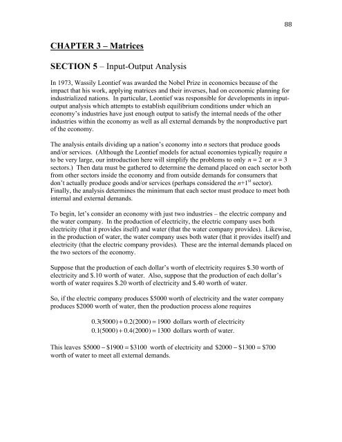
CHAPTER 3 â Matrices SECTION 5 â Input-Output Analysis
CHAPTER 3 â Matrices SECTION 5 â Input-Output Analysis
CHAPTER 3 â Matrices SECTION 5 â Input-Output Analysis
Create successful ePaper yourself
Turn your PDF publications into a flip-book with our unique Google optimized e-Paper software.
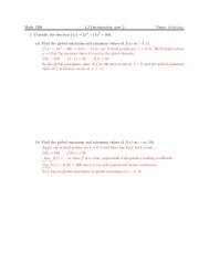
92The production matrix is⎡ x ⎤⎢ ⎥y⎣⎢⎦⎥ = ( I − C)−1E⎡⎢= ⎢⎢⎢⎣34− 1 3⎡ 80⎢57= ⎢⎢ 10⎢⎣ 19− 110893 ⎤⎥19 ⎥⎡45 ⎥⎢⎣⎥38 ⎦⎤⎥⎥⎡⎥⎢⎣⎥⎦50010005001000⎤⎥⎦⎡⎤⎢⎥ = ⎢⎦ ⎢⎢⎣49000572750019⎤⎥⎥⎡=⎥⎢⎣⎥⎦8601447⎤⎥⎦In order to satisfy the demand, production of 860 metric tons ofwheat is required and 1447 metric tons of oil is required.Example 3.5.3:Solution:An economy of a small island nation is based on three sectors:agriculture, energy, and manufacturing. The production of adollar’s worth of agriculture requires an input of $0.20 from theagriculture sector and $0.40 from the energy sector. Theproduction of a dollar’s worth of energy requires an input of $0.20from the energy sector and $0.40 from the manufacturing sector.The production of a dollar’s worth of manufacturing requires inputof $0.10 from the agriculture sector, $0.10 from the energy sector,and $0.30 from the manufacturing sector.Find the output required of each sector to meet a demand (external)of $20 billion for agriculture, $10 billion for energy, and $30billion for manufacturing.In class
93<strong>CHAPTER</strong> 3 – <strong>Matrices</strong><strong>SECTION</strong> 6 – Cramer’s RuleTo finish off our discussion of matrices, we will look at one last method to solving asystem of linear equations. Cramer’s rule provides a method to solve a system of linearequations when there is one unique solution and the number of variables is equal to thenumber of equations.Cramer’s rule does have the same downfall as the method using the inverse of thecoefficient matrix to solve a system (seen in Chapter 3, Section 4), in that the rule cannotdistinguish between a system with “no solution” and “infinitely many solutions”. It isonly useful when there is exactly one solution to the system.To use Cramer’s rule, we first need to be able to compute the determinant of a squarematrix.Notation: Determinant of a matrixFor a square matrix A, the determinant of the matrix is written det A ( ) or A .For a 2 × 2 matrix the determinant isa bc dthat we use to find the inverse of a 2 × 2 matrix.= ad − bc . This is precisely the value DFor larger square matrices, the determinant can be defined recursively. That is, to findthe determinant of a 3 × 3 matrix, we use determinants of certain 2 × 2 submatrices. Tofind the determinant of a 4 × 4 matrix, we use determinants of certain 3 × 3 submatrices.The pattern continues.Definition: Submatrix of a ijThe matrix that remains when the entire i th row and entire j th column areeliminated is called the submatrix of the entry a ij.We will denote the submatrix of the entry a ijwith the notation M ij.Example 3.6.1:Determine each of the following submatrices for the matrix⎡ 6 −2 5 ⎤⎢⎥A =⎢8 1 7⎥.⎣⎢−3 2 0 ⎦⎥a.) M 11b.) M 32
97Again, it is important to realize that when D = 0 , we cannot apply Cramer’s Rule. Thiswill happen when the system has no solution or infinitely many solutions. Unfortunately,we cannot tell which case it is though and to determine that, we must try a differentmethod of solving.Example 3.6.6:Solution:Use Cramer’s Rule to solve the system.⎧x + 2y = 10⎪⎨3x + 4z = 7 .⎪⎩−y − z = 1In class


