Lecture Notes on Integral Calculus - Ugrad.math.ubc.ca

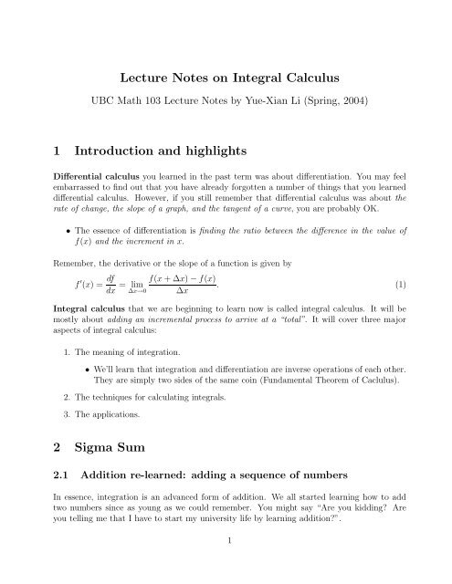
2.3 The sigma notationIn order to short-hand the mathematical exression of the sum of a regular sequence, a convenientnotation is introduced.Definition (Σ sum): The sum of the first k terms of a sequence generated by the sequencegenerator f(i) can be denoted byS k = f(1) + f(2) + · · · + f(k) ≡k∑f(i)i=1where the symbol Σ (the Greek equivalent of S reads “sigma”) means “take the sum of”,the general expression for the terms to be added or the sequence generator f(i) is called thesummand, i is called the summation index, 1 and k are, respectively, the starting and theending indices of the sum.Thus,k∑f(i)i=1means calculate the sum of all the terms generated by the sequence generator f(i) for all integersstarting from i = 1 and ending at i = k.Note that the value of the sum is independent of the summation index i, hence i is called a“dummy” variable serving for the sole purpose of running the summation from the startingindex to the ending index. Therefore, the sum only depends on the summand and both thestarting and the ending indices.∑Example 5: Express the sum S k = k i 2 in an expanded form.i=3Solution 5: The sequence generator is f(i) = i 2 . Note that the starting index is not 1 but 3!.Thus, the 1st term is f(3) = 3 2 . The subsequent terms can be determined accordngly. Thus,S k =k∑i 2 = f(3) + f(4) + f(5) + · · · + f(k) = 3 2 + 4 2 + 5 2 + · · · + k 2 .i=3An easy check for a mistake that often occurs. If you still find the “dummy” variable i in anexpanded form or in the final evaluation of the sum, your answer must be WRONG.2.4 Gauss’s formula and other formulas for simple sumsLet us return to Examples 1 and 2 about the total number of logs in a triangular pile. Let’sstart with a pile of 4 layers. Imaging that you could (in a “thought-experiement”) put an4

identical pile with up side down adjacent to the original pile, you obtain a pile that containstwice the number of logs that you want to calculate (see figure).The advantage of doing this is that, in this double-sized pile, each layer contains an equalnumber of logs. This number is equal to number on the 1st (top) layer plus the number on the4th (bottom) layer. In the mean time, the height of the pile remains unchanged (4). Thus, thenumber in this double-sized pile is 4 × (4 + 1) = 20. The sum S 4 is just half of this numberwhich is 10.Let’s apply this idea to finding the formula in the case of k layers. Note that(Original) S k = 1 + 2 + · · · + k − 1 + k. (2)(Inversed) S k = k + k − 1 + · · · + 2 + 1. (3)(Adding the two) 2S k = (k + 1) + (k + 1) + · · · + (k + 1) + (k + 1) = k(k + 1).} {{ }(4)k terms in totalDividing both sides by 2, we obtain Gauss’s formula for the sum of the first k positive integers.S k =k∑i=1i = 1 + 2 + · · · + k = 1 k(k + 1). (5)2This actaully answered the problem in Example 2. The answer to Example 1b is even simpler.S 50 =50∑i=1i = 1 × 50 × 51 = 1275.2The following are two important simple sums that we shall use later. One is the sum of thefirst k integers squared.S k =k∑i=1i 2 = 1 2 + 2 2 + · · · + k 2 = 1 k(k + 1)(2k + 1). (6)6The other is the sum of the first k integers cubed.S k =k∑[ ] 2 1i 3 = 1 3 + 2 3 + · · · + k 3 =2 k(k + 1) . (7)i=1We shall not illustrate how to derive these formulas. You can find it in numerous calculus textbooks.To prove that these formulas work for arbitrarily large integers k, we can use a method calledmathematical induction. To save time, we’ll just outline the basic ideas here.5

The only way we can prove things concerning arbitrarily large numbers is to guarantee thatthis formula must be correct for k = N + 1 if it is correct for k = N. This is like tryingto arrange a string/sequence of standing dominos. To guarantee that all the dominos in thestring/sequence fall one after the other, we need to guarantee that the falling of each dominowill necessarily cause the falling of the subsequent one. This is the essence of proving that ifthe formula is right for k = N, it must be right for k = N + 1. The last thing you need to dois to knock down the first one and keep your fingers crossed. Knocking down the first dominois equivalent to proving that the formula is correct for k = 1 which is very easy to check in allcases (see Keshet’s notes for a prove of the sum of the first k integers squared).2.5 Important rules of sigma sumsRule 1: Summation involving constant summand.k∑i=1c = c}+ c +{{· · · +}c = kc.k terms in totalNote that: the total # of terms=ending index - starting index +1.Rule 2: Constant multiplication: multiplying a sum by a constant is equal to multiplying eachterm of the sum by the same constant.k∑c f(i) =i=1k∑cf(i)i=1Rule 3: Adding two sums with identical starting and ending indices is equal to the sum of sumsof the corresponding terms.k∑f(i) +i=1k∑g(i) =i=1k∑[f(i) + g(i)].i=1Rule 4: Break one sum into more than one pieces.k∑f(i) =i=1n∑k∑f(i) + f(i),i=1 i=n+1(1 ≤ n < k).Example 7: Let’s go back to solve the sum of the first k odd numbers.Solution 7:k∑k∑ k∑O k = 1 + 3 + · · · + (2k − 1) = (2i − 1) = (2i) − 1 = 2111k∑i − k,16

where Rules 1, 2, and 3 are used in the last two steps. Using the known formulas, we obtainO k =k∑(2i − 1) = k(k + 1) − k = k 2 .1Example 8: Let us now go back to solve Example 4. It is the sum of the first k products ofpairs of subsequent integers.Solution 8:P k = 1 · 2 + 2 · 3 + · · · + k · (k + 1) =k∑i(i + 1) =1k∑[i 2 + i] =where Rule 3 was used in the last step. Applying the formulas, we learnedP k =k∑11k∑i 2 +i(i + 1) = 1 6 k(k + 1)(2k + 1) + 1 2 k(k + 1) = 1 k(k + 1)(k + 2).3This is another simple sum that we can easily remember.∑Example 9: Calculate the sum S = k (i + 2) 3 .11k∑i,Solution 9: This problem can be solved in two different ways. The first is to expand thesummand f(i) = (i + 2) 3 which yieldS =k∑(i + 2) 3 =1k∑(i 3 + 6i 2 + 12i + 8) =1k∑i 3 + 61k∑i 2 + 12We can solve the resulting three sums separately using the known formulas.11k∑i + 8k.But there is a better way to solve this. This involves substituting the summation index. Wefind it easier to see how substitution works by expanding the sum.S =k∑(i + 2) 3 = 3 3 + 4 3 + · · · + k 3 + (k + 1) 3 + (k + 2) 3 .i=1We see that this is simply a sum of integers cubed. But the sum does not start at 1 3 and endat k 3 like in the formula for the sum of the first k integers cubed.Thus we re-write the sum with a sigma notation with an new index called l which starts atl = 3 and ends at l = k + 2 (there is no need to change the symbol for the index, you can keepcalling it i if you do not feel any confusion). Thus,1S =k∑∑k+2(i + 2) 3 = 3 3 + 4 3 + · · · + k 3 + (k + 1) 3 + (k + 2) 3 = l 3 .i=1l=37

We just finished doing a substitution of the summation index. It is equivalent to replacing iby l = i + 2. This relation also implies that i = 1 ⇒ l = 3 and i = k ⇒ l = k + 2. This isactually how you can determine the starting and the ending values of the new index.Now we can solve this sum using Rule 4 and the known formula.S =k∑ ∑k+2∑k+22∑[ ] 2 [ ] 2 1 1(i+2) 3 = l 3 = l 3 − l 3 =2 (k + 2)(k + 3) −1 2 −2 3 =2 (k + 2)(k + 3) −9.i=1l=3 l=1 l=12.6 Applications of sigma sumThe area under a curveWe know that the area of a rectangle with length l and width w is A rect = w · l.Starting from this formula we can calculate the area of a triangle and a trapezoid. This isbecause a triangle and a trapezoid can be transformed into a rectangle (see Figure). Thus, fora triangle of height h and base length bA trig = 1 2 hb.Similarly, for a trapezoid with base length b, top length t, and height hA trap = 1 h(t + b).2Following a very similar idea, the sum of a trapezoid-shaped pile of logs with t logs on toplayer, b logs on the bottom layer, and a height of h = b − t + 1 layers (see figure) isb∑i=ti = t + (t + 1) + · · · + (b − 1) + b = 1 2 h(t + b) = 1 (b − t + 1)(t + b). (8)2Now returning to the problem of calculating the area. Another important formula is for thearea of a circle of radius r.A circ = πr 2 .Now, once we learned sigma and/or integration, we can calculate the area under the curve ofany function that is integrable.Example 10: Calculate the area under the curve y = x 2 between 0 and 2 (see figure).Solution 10: Remember always try to reduce a problem that you do not know how to solveinto a problem that you know how to solve.8

Let the area be A. Let’s divide A into 3 rectangles of equal width w = 2/3. Thus,{w[xA ≈ w·h 1 +w·h 2 +w·h 3 =2 0 + x2 1 + x2 2 ] = 1 3 [02 + ( )1 2+ ( 2 23 3)], left − end approx.;w[x 2 1 + x2 2 + x2 3 ] = 1[( )1 2+ ( )2 2+ ( 3 23 3 3 3)], right − end approx..By using these rectangles, we introduced large errors in our estimates using the heights basedon both the left and the right endpoints of the subintervals. To increase accurary, we need toincrease the number of rectangles by making each one thinner. Let us now divide A into nrectangles of equal width w = 2/n. Thus, using the height based on the right endpoint of eachsubinterval, we obtainA ≈ S n = A 1 + A 2 + · · · + A n =n∑w · h i = wi=1n∑f(x i ) = 2 ni=1n∑x 2 i .i=1It is very important to keep a clear account of the height of each rectangle. In this case,h i = f(x i ) = x 2 i . Thus, the key is finding the x-coordinate of the right-end of each rectangle.For rectangles of of equal width, x i = x 0 + iw = x 0 + i∆x/n, where ∆x is the length of theinterval x 0 is the left endpoint of the interval. x 0 = 0 and ∆x = 2 for this example. Therefore,x i = i(2/n). Substitute into the above equationA ≈ S n = 2 nn∑x 2 i . = 2 ni=1n∑i=1( ) 2 2i= 8 n∑i 2 = 8 1n n 3 n 3 6 n(n + 1)(2n + 1) = 4 (n + 1)(2n + 1).3 n 2 i=1Note that if we divide the area into infinitely many retangles with a width that is infinitelysmall, the approximate becomes accurate.A = limn→∞S n = lim3n→∞4The volume of a solid revolution of a curve(n + 1)(2n + 1)n 2 = 8 3 .We know the volume of a rectangular block of height h, width w, and length l isV rect = w · l · h.The volume of a cylinder of thichness h and radius rV cyl = A cross · h = πr 2 h.Example 11: Calculate the volume of the bowl-shaped solid obtained by rotating the curvey = x 2 on [0, 2] about the y-axis.9

2.7 The sum of a geometric sequence3 The Definite Integrals and the Fundamental Theorem3.1 Riemann sumsDefinition 1: Suppose f(x) is finite-valued and piecewise continuous on [a, b]. Let P ={x 0 = a, x 1 , x 2 , . . . , x n = b} be a partition of [a, b] into n subintervals I i = [x i−1 , x i ] of width∆x i = x i − x i−1 , i = 1, 2, . . . , n. (Note in a special case, we can partition it into subintervalsof equal width: ∆x i = x i − x i−1 = w = (b − a)/n for all i). Let x ∗ i be a point in I i such thatx i−1 ≤ x ∗ i ≤ x i . (Here are some special ways to choose x ∗ i : (i) left endpoint rule x∗ i = x i−1 ,and (ii) the right endpoint rule x ∗ i = x i ).The Riemann sums of f(x) on the interval [a, b] are defined by:n∑n∑R n = h i ∆x i = f(x ∗ i )∆x ii=1which approximate the area between f(x) and the x-axis by the sum of the areas of n thinrectangles (see figure).Example 1: Approximate the area under the curve of y = e x on [0, 1] by 10 rectangles ofequal width using the left endpoint rule.Solution 1: We are actually calculating the Riemann sum R 10 . The width of each rectangleis ∆x i = w = 1/10 = 0.1 (for all i). The left endpoint of each subinterval is x ∗ i = x i − 1 =(i − 1)/10. Thus,R 10 =10∑i=1f(x ∗ i )∆x i =10∑i=1i=1e (i−1)/10 (0.1) = 0.19∑e j/10 = 0.11 − e ≈ 1.6338.1 − e1/10 j=03.2 The definite integralDefinition 1: Suppose f(x) is finite-valued and piecewise continuous on [a, b]. Let P = {x 0 =a, x 1 , x 2 , . . . , x n = b} be a partition of [a, b] with a length defined by |p| = Max 1≤i≤n {∆x i }(i.e. the longest of all subintervals). The definite integral of f(x) on [a, b] is∫ baf(x)dx =lim R n =|p|→0; n→∞lim|p|→0; n→∞n∑f(x ∗ i )∆x iwhere the symbol ∫ means “to integrate”, the function f(x) to be integrated is called theintegrand, x is called the integration variable which is a “dummy” variable, a and b are,i=110

espectively, the lower (or the starting) limit and the upper (or the ending) limit of the integral.Thus,∫ baf(x)dxmeans integrate the function f(x) starting from x = a and ending at x = b.Example 2: Calculate the definite integral of f(x) = x 2 on [0.2]. (This is Example 10 of<strong>Lecture</strong> 1 reformulated in the form of a definite integral).Solution 2:I =∫ 20x 2 dx = limn→∞n∑( 2ini=1) 2} {{ }f(x ∗ i )( ) 2n} {{ }∆x i( ) n∑ 8= lim i 2 = limn→∞ n 3 i=13n→∞4(n + 1)(2n + 1)n 2 = 8 3 .Important remarks on the relation between an area and a definite integral:• An area, defined as the physical measure of the size of a 2D domain, is always nonnegative.• The value of a definite integral, sometimes also referred to as an “area”, can be bothpositive and negative.• This is because: a definite integral = the limit of Riemann sums. But Riemann sumsare defined asn∑n∑R n = (area of i th rectangle) = f(x ∗ i ) ∆x} {{ } i . }{{}i=1i=1height width• Note that both the hieght f(x ∗ i ) and the width ∆x i can be negative implying that R ncan have either signs.3.3 The fundamental theorem of calculus3.4 Areas between two curves11

4 Applications of Definite Integrals: I4.1 Displacement, velocity, and acceleration4.2 Density and total mass4.3 Rates of change and total change4.4 The average value of a function12

5 DifferentialsDefinition: The differential, dF , of any differentiable function F is an infinitely small incrementor change in the value of F .Remark: dF is measured in the same units as F itself.Example: If x is the position of a moving body measured in units of m (meters), then itsdifferential, dx, is also in units of m. dx is an infinitely small increment/change in the positionx.Example: If t is time measured in units of s (seconds), then its differential, dt, is also in unitsof s. dt is an infinitely small increment/change in time t.Example: If A is area measured in units of m 2 (square meters), then its differential, dA, alsois in units of m 2 . dA is an infinitely small increment/change in area A.Example: If V is volume measured in units of m 3 (cubic meters), then its differential, dV ,also is in units of m 3 . dV is an infinitely small increment/change in volume V .Example: If v is velocity measured in units of m/s (meters per second), then its differential,dv, also is in units of m/s. dv is an infinitely small increment/change in velocity v.Example: If C is the concentration of a biomolecule in our body fluid measured in units ofM (1 M = 1 molar = 1 mole/litre, where 1 mole is about 6.023 × 10 23 molecules), thenits differential, dC, also is in units of M. dC is an infinitely small increment/change in theconcentration C.Example: If m is the mass of a rocket measured in units of kg (kilograms), then its differential,dm, also is in units of kg. dm is an infinitely small increment/change in the mass m.Example: If F (h) is the culmulative probability of finding a man in Canada whose height issmaller than h (meters), then dF is an infinitely small increment in the probability.Definition: The derivative of a function F with respect to another function x is defined asthe quotient between their differentials:13

dFdx=an infinitely small rise in Fan infinitely small run in x .Example: Velocity as the rate of change in position x with respect to time t can be expressedasv =infinitely small change in positioninfinitely small time interval= dxdt .Remark: Many physical laws are correct only when expressed in terms of differentials.Example: The formula (distance) = (velocity) × (time interval) is true either when thevelocity is a constant or in terms of differentials, i.e., (an infinitely small distance) =(velocity) × (an infinitely short time interval). This is because in an infinitely short timeinterval, the velocity can be considered a constant. Thus,which is nothing new but v(t) = dx/dt.dx = dx dt = v(t)dt,dtExample: The formula (work) = (force) × (distance) is true either when the forceis a constant or in terms of differentials, i.e., (an infinitely small work) = (force) ×(an infinitely small distance). This is because in an infinitely small distance, the force canbe considered a constant. Thus,dW = fdx = f dx dt = f(t)v(t)dt,dtwhich simply implies: (1) f = dW/dx, i.e., force f is nothing but the rate of change in workW with respect to distance x; (2) dW/dt = f(t)v(t), i.e., the rate of change in work W withrespect to time t is equal to the product between f(t) and v(t).Example: The formula (mass) = (density) × (volume) is true either when the densityis constant or in terms of differentials, i.e., (an infinitely small mass) = (density) ×14

(volume of an infinitely small volume). This is because in an infinitely small piece ofvolume, the density can be considered a constant. Thus,dm = ρdV,which implies that ρ = dm/dV , i.e., density is nothing but the rate of change in mass withrespect to volume.6 The Chain Rule in Terms of DifferentialsWhen we differentiate a composite function, we need to use the Chain Rule. For example,f(x) = e x2 is a composite function. This is because f is not an exponential function of x butit is an exponential function of u = x 2 which is itself a power function of x. Thus,dfdx = dex2dx = deu dudx du = (deu du )(du dx ) = eu (x 2 ) ′ = 2xe x2 ,where a substitution u = x 2 was used to change f(x) into a true exponential function f(u).Therefore, the Chain Rule can be simply interpreted as the quotient between df and dx is equalto the quotient between df and du multiplied by the quotient between du and dx. Or simply,divide df/dx by du and then multiply it by du.However, if we simply regard x 2 as a function different from x, the actual substitution u = x 2becomes unnecessary. Instead, the above derivative can be expressed asde x2dx = dx 2 dex2dx dx = 2 (dex2 dx 2 )(dx2 dx ) = (x 2 ) ′ = 2xe ex2 x2 .Generally, if f = f(g(x)) is a differentiable function of g and g is a differentiable function ofx, thendfdx = df dgdg dx ,where df, dg, and dx are, respectively, the differentials of the functions f, g, and x.Example: Calculate df/dx for f(x) = sin(ln(x 2 + e x )).Solution: f is a composite function of another composite function!15

dfdx = d sin(ln(x2 + e x ))d ln(x 2 + e x )d ln(x 2 + e x ) d(x 2 + e x )d(x 2 + e x ) dx= cos(ln(x 2 + e x 1))(x 2 + e x ) (2x + ex ).7 The Product Rule in Terms of DifferentialsThe Product Rule says if both u = u(x) and v = v(x) are differentiable functions of x, thend(uv)dx= v dudx + udv dx .Multiply both sides by the differential dx, we obtaind(uv) = vdu + udv,which is the Product Rule in terms of differentials.Example: Let u = x 2 and v = e sin(x2) , thend(uv) = vdu + udv = e sin(x2) d(x 2 ) + x 2 d(e sin(x2) )= 2xe sin(x2) dx + x 2 e sin(x2) cos(x 2 )(2x)dx = 2xe sin(x2) [1 + x 2 cos(x 2 )]dx.8 Other Properties of Differentials1. For any differentiable function F (x), dF = F ′ (x)dx (Recall that F ′ (x) = dF/dx!).2. For any constant C, dC = 0.3. for any constant C and differentiable function F (x), d(CF ) = CdF = CF ′ (x)dx.4. For any differentiable functions u and v, d(u ± v) = du ± dv.16

9 The Fundamental Theorem in Terms of DifferentialsFundamental Theorem of Calculus: If F (x) is one antiderivative of the function f(x), i.e.,F ′ (x) = f(x), then∫∫f(x)dx =∫F ′ (x)dx =dF = F (x) + C.Thus, the integral of the differential of a function F is equal to the function itselfplus an arbitrary constant. This is simply saying that differential and integral are inversemath operations of each other. If we first differentiate a function F (x) and then integrate thederivative F ′ (x) = f(x), we obtain F (x) itself plus an arbitrary constant. The opposite also istrue. If we first integrate a function f(x) and then differentiate the resulting integral F (x)+C,we obtain F ′ (x) = f(x) itself.Example:∫∫x 5 dx =d( x66 ) = x66 + C.Example:∫∫e −x dx =d(−e −x ) = −e −x + C.Example:∫∫cos(3x)dx =d( sin(3x) ) = sin(3x) + C.3 3Example:∫∫sec 2 xdx =dtanx = tanx + C.Example:∫∫cosh(3x)dx =d( sinh(3x) ) = sinh(3x) + C.3317

Example:∫∫11 + x dx = 2dtan −1 x = tan −1 + C.Example:∫∫11 − tanh 2 x dx =∫ 1 + cosh(2x)=dx = 1 ∫22∫1sech 2 x dx =cosh 2 xdxd(x + sinh(2x) ) = 1 sinh(2x)[x + ] + C.2 2 2For more indefinite integrals involving elementary functions, look at the first page of the tableof integrals provided at the end of the notes.10 Integration by SubsitutionSubstitution is a necessity when integrating a composite function since we cannot write downthe antiderivative of a composite function in a straightforward manner.Many students find it difficult to figure out the substitution since for different functions thesubsitutions are also different. However, there is a general rule in substitution, namely, tochange the composite function into a simple, elementary function.Example: ∫ (sin( √ x)/ √ x)dx.Solution: Note that sin( √ x) is not an elementary sine function but a composite function. Thefirst goal in solving this integral is to change sin( √ x) into an elementary sine function throughsubstitution. Once you realize this, u = √ x is an obvious subsitution. Thus, du = u ′ dx =12 √ x dx, or dx = 2√ xdu = 2udu. Substitute into the integral, we obtain∫ sin(√ x)√ xdx =∫ sin(u)u∫2udu = 2∫sin(u)du = −2dcos(u) = −2cos(u)+C = −2cos( √ x)+C.Once you become more experienced with subsitutions and differentials, you do not need to dothe actual substitution but only symbolically. Note that x = ( √ x) 2 ,18

∫ √ ∫ √ sin( x) sin( x)√ dx = √ d( √ ∫ √ sin( x)x) 2 = √ 2 √ xd √ ∫x = 2x x xsin( √ x)d √ x = −2cos( √ x)+C.Thus, as soon as you realize that √ x is the substitution, your goal is to change the differentialin the integral dx into the differential of √ x which is d √ x.If you feel that you cannot do it without the actual substitution, that is fine. You can alwaysdo the actual substitution. I here simply want to teach you a way that actual subsitution is nota necessity!Example: ∫ x 4 cos(x 5 )dx.Solution: Note that cos(x 5 ) is a composite function that becomes a simple cosine function onlyif the subsitution u = x 5 is made. Since du = u ′ dx = 5x 4 dx, x 4 dx = 1 du. Thus,5Or alternatively,∫x 4 cos(x 5 )dx = 1 5∫cos(u)du = sin(u)5+ C = sin(x5 )5+ C.∫x 4 cos(x 5 )dx = 1 5∫cos(x 5 )dx 5 = 1 5 sin(x5 ) + C.Example: ∫ x √ x 2 + 1dx.Solution: Note that √ x 2 + 1 = (x 2 + 1) 1/2 is a composite function. We realize that u = x 2 + 1is a substitution. du = u ′ dx = 2xdx implies xdx = 1 du. Thus,2Or alternatively,∫x √ x 2 + 1dx = 1 ∫ √udu 1 2 =22 3 u3/2 + C = (x2 + 1) 3/23+ C.∫x √ x 2 + 1dx = 1 2∫ √x2+ 1d(x 2 + 1) = 1 22 3 (x2 + 1) 3/2 + C = (x2 + 1) 3/2+ C.319

In many cases, substitution is required even no obvious composite function is involved.Example: ∫ (ln x/x)dx (x > 0).Solution: The integrand ln x/x is not a composite function. Nevertheless, its antiderivative isnot obvious to calculate. We need to figure out that (1/x)dx = d ln x, thus by introducing thesubstitution u = ln x, we obtained a differential of the function ln x which also appears in theintegrand. Therefore,∫∫(ln x/x)dx =udu = u22 + C = 1 2 (ln x)2 + C.It is more natural to consider this substitution is an attempt to change the differential dx intosomething that is identical to a function that appears in the integrand, namely d ln x. Thus,∫∫(ln x/x)dx =ln xd ln x = 1 2 (ln x)2 + C.Example: ∫ tan xdx.Solution: tan x is not a composite function. Nevertheless, it is not obvious to figure out tan xis the derivative of what function. However, if we write tan x = sin x/ cos x, we can regard1/ cos x as a composite function. We see that u = cosx is a candidate for substitution anddu = u ′ dx = −sin(x)dx. Thus,∫tanxdx =∫ sinxcosx dx = − ∫ duu= − ln |u| + C = − ln |cosx| + C.Or alternatively,∫tanxdx =∫ ∫ sinx dcosxcosx dx = − cosx= − ln |cosx| + C.Some substitutions are standard in solving specific types of integrals.Example: Integrands of the type (a 2 − x 2 ) ±1/2 .In this case both x = asinu and x = acosu will be good. x = a tanh u also works (1−tanh 2 u =sech 2 u). Let’s pick x = asinu in this example. If you ask how can we find out that x = asinu20

is the substitution, the answer is a 2 −x 2 = a 2 (1−sin 2 u) = a 2 cos 2 u. This will help us eliminatethe half power in the integrand. Note that with this substitution, u = sin −1 (x/a), sinu = x/a,and cosu = √ 1 − x 2 /a 2 . Thus,∫∫dx√a2 − x = 2∫ ∫d(asinu) acosudu√a2 − a 2 sin 2 u = acosu=du = u + C = sin −1 x a + C.Note that ∫ dx/ √ 1 − x 2 = sin −1 x + C, we can make a simple substitution x = au, thus∫∫dx√a2 − x = 2∫d(au)√a2 − a 2 u = 2du√1 − u2 = sin−1 u + C = sin −1 x a + C.Similarly,∫ √a2∫ √a2∫− x 2 dx = − a 2 sin 2 ud(asinu) = a 2∫ 1 + cos(2u)cos 2 udu = a 2 du2= a22sin(2u)[u + ] + C = a222 [u + sinucosu] + C = 1 2 [a2 sin −1 ( x a ) + x√ a 2 − x 2 ] + C.Example: Integrands of the type (a 2 + x 2 ) ±1/2 .x = asinh(u) is a good substitution since a 2 + x 2 = a 2 + a 2 sinh 2 (u) = a 2 (1 + sinh 2 (u)) =a 2 cosh 2 (u), where the hyperbolic identity 1 + sinh 2 (u) = cosh 2 (u) was used. (x = a tan u isalso good since 1 + tan 2 u = sec 2 u!). Thus,∫∫dx√a2 + x = 2∫ ∫dasinh(u) acosh(u)du√a2 + a 2 sinh 2 (u) = =acosh(u)du = u + C = sinh −1 ( x a ) + C= ln |x + √ a 2 + x 2 | + C,where sinh −1 (x/a) = ln |x + √ a 2 + x 2 | − ln |a| was used. And,∫ √a2∫ √a2∫+ x 2 dx = + a 2 sinh 2 (u)dasinh(u) = a 221cosh 2 (u)du = a22∫[1 + cosh(2u)]du

= a2 sinh(2u)[u + ] + C = 1 2 22 [a2 sinh −1 ( x a ) + a2 sinh(u)cosh(u)] + C= 1 2 [a2 ln |x + √ a 2 + x 2 | + x √ a 2 + x 2 ] + C,where the following hyperbolic identities were used: sinh(2u) = 2sinh(u)cosh(u), sinh −1 (x/a) =ln |x + √ a 2 + x 2 | − ln |a|, and acosh(u) = √ a 2 + x 2 .Example: Integrands of the type (x 2 − a 2 ) ±1/2 .x = acosh(u) is prefered since x 2 − a 2 = a 2 scos 2 (u) − a 2 = a 2 [cosh 2 (u) − 1] = a 2 sinh 2 (u),where the hyperbolic identity cosh 2 (u)−1 = sinh 2 (u) was used. (x = a sec u is also good sincesec 2 u − 1 = tan 2 u!). Thus,∫∫dx√x2 − a = 2∫ ∫da cosh(u) a sinh(u)du==√a 2 cosh 2 (u) − a 2 a sinh(u)du = u + C= cosh −1 ( x a ) + C = ln |x + √ x 2 − a 2 | + C.Similarly∫ √x2− a 2 dx =∫ √a 2 cosh 2 (u) − a 2 da cosh(u) = a 2 ∫sinh 2 udu = a22∫[cosh(2u) − 1]du= 1 2 [x√ x 2 − a 2 − a 2 ln |x + √ x 2 − a 2 |] + C,where cosh u = x/a, sinh u = √ x 2 /a 2 − 1, and u = ln |x + √ x 2 − a 2 | − ln a were used.For more details on hyperbolic functions, read the last page of the table of integrals at the endof the notes.More Exercises on Substitution:22

1. Substitution aimed at eliminating a composite functionExample:(i)∫∫ √ 4xd(2x 2 ∫32x 2 + 3 dx = √ + 3)32x 2 + 3 =u −1/3 du = 3 2 u2/3 + C = 3 2 (2x2 + 3) 2/3 + C.(ii)∫x√ dx = 1 ∫ 2x + 3 − 3√ d(2x + 3) = 1 ∫ u − 32x + 3 4 2x + 3 4 u du = 1 ∫1/2 4[u 1/2 − 3u −1/2 ]du= 1 4 [2 3 u3/2 − 6u 1/2 ] + C = 1 4 [2 3 (2x + 3)3/2 − 6(2x + 3) 1/2 ] + C.Edwards/Penney 5 th − ed 5.7 Problems.∫∫(1) (3x − 5) 17 dx (3)∫(7)∫(23)∫x sin(2x 2 )dx (9)x √ ∫2 − 3x 2 dx (31)x √ ∫x 2x 2 + 9dx (4) √ 32x 3 − 1 dx∫(1 − cosx) 5 dxsinxdx (15) √ dx 7x + 5∫cos 3 xsinxdx (33)tan 3 xsec 2 xdx(45)∫ cos(√ x)√ xdx (49)∫π/20(1 + 3sinθ) 3/2 cosθdθ (51)∫π/20e sinx cosxdxEdwards/Penney 5 th − ed 9.2 Problems.(7)∫(21)∫ √ √ ∫cot( y)csc( y)√ dy (11)ytan 4 (3x)sec 2 (3x)dx (25)∫ (ln t)e −cotx csc 2 1 0xdx (13) dt, (t > 0)t∫ √ (1 + x)4∫√ dx (31) x 2√ x + 2dx.x2. Substitution to achieve a function in differential that appears in the integrand23

Example:(i) ∫e x ∫1 + e dx = 2xde x ∫1 + (e x ) = 2du1 + u 2 = tan−1 (u) + C = tan −1 (e x ) + C.(ii)∫x√e2x 2 − 1 dx = 1 ∫2dx 2√e2x 2 (1 − e −2x2 ) = 1 ∫2du√e2u(1 − e −2u ) = 1 ∫2due u√ 1 − (e −u ) 2= − 1 2∫de −u ∫√1 − (e−u) = −1 2 2dy√1 − y2 = 1 2 cos−1 (y)+C = 1 2 cos−1 (e −u )+C = 1 2 cos−1 (e −x2 )+C.Edwards/Penney 5 th − ed 9.2 Problems (difficult ones!).∫(17)sinθ)∫(27)e 2x∫1 + e dy, (u = 4x e2x ) (19)∫1(1 + t 2 )tan −1 t dt, (u = tan−1 t) (29)∫3x√ dx, (u = 1 − x4 x2 ) (23)1√e2x− 1 dx, (u = e−x )cosθdθ, (u =1 + sin 2 θ3. Special Trigonometric SubstitutionsExample:(i)∫x 3 ∫√ dx = 1 − x2sin 3 ∫ud sin u√1 − sin 2 u =∫sin 3 udu = −(1 − cos 2 u)d cos u= cos3 u3− cos u + C = (1 − x2 ) 3/23− √ 1 − x 2 + C.Edwards/Penney 5 th − ed 9.6 Problems (difficult ones!).∫∫ √ ∫1(1) √ dx, (x = 4 sin u) (9) x2 − 1dx, (x = cosh u) (11)16 − x2 x3 sinh u)x 3√ 9 + 4x 2 dx, (2x =24

∫ √ ∫1 − 4x2(13)dx, (2x = sin u) (19)x3 sinh u)x 2√1 + x2 dx, (x = sinh u) (27) ∫ √9+ 16x2 dx, (4x =11 Integration by PartsIntegration by Parts is the integral version of the Product Rule in differentiation. The ProductRule in terms of differentials reads,Integrating both sides, we obtaind(uv) = vdu + udv.∫∫d(uv) =∫vdu +udv.Note that ∫ d(uv) = uv + C, the above equation can be expressed in the following form,∫∫udv = uv −vdu.Generally speaking, we need to use Integration by Parts to solve many integrals that involvethe product between two functions. In many cases, Integration by Parts is most efficient insolving integrals of the product between a polynomial and an exponential, a logarithmic, or atrigonometric function. It also applies to the product between exponential and trigonometricfunctions.Example: ∫ xe x dx.Solution: In order to eliminate the power function x, we note that (x) ′ = 1. Thus,∫∫xe x dx =∫xde x = xe x −e x dx = xe x − e x + C.Example: ∫ x 2 cosxdx.Solution: In order to eliminate the power function x 2 , we note that (x 2 ) ′′ = 2. Thus, we needto use Integration by Patrs twice.25

∫∫x 2 cosxdx =∫x 2 dsinx = x 2 sinx −∫sinxdx 2 = x 2 sinx −2xd(−cosx)∫= x 2 sinx + 2∫xdcosx = x 2 sinx + 2xcosx − 2cosxdx = x 2 sinx + 2xcosx − 2sinx + C.Example: ∫ x 2 e −2x dx.Solution: In order to eliminate the power function x 2 , we note that (x 2 ) ′′ = 2. Thus, we needto use Integration by Patrs twice. However, the number (−2) can prove extremely annoyingand easily cause errors. Here is how we use substitution to avoid this problem.∫x 2 e −2x dx = −12 3 ∫(−2x) 2 e −2x d(−2x) = −18∫u 2 e u du = −1 ∫8 [u2 e u − 2ue u du]= −18 [u2 e u − 2(ue u − e u )] + C = −eu8 [u2 − 2u + 2] + C = −e−2x[4x 2 + 4x + 2] + C.8When integrating the product between a polynomial and a logarithmic function, the main goalis to eliminate the logarithmic function by differentiating it. This is because (ln x) ′ = 1/x.Example: ∫ ln xdx, (x > 0).Solution:∫∫ln xdx = x ln x −∫xd ln x = x ln x −x dx x= x ln x − x + C.Example: ∫ x(ln x) 2 dx, (x > 0).Solution:∫x(ln x) 2 dx = 1 2∫(ln x) 2 dx 2 = 1 ∫2 [x2 (ln x) 2 −x 2 (2 ln x) dx x ] = 1 ∫2 [x2 (ln x) 2 −ln xdx 2 ]26

= 1 2 [x2 (ln x) 2 − x 2 ln x + x22 ] + C = x22 [(ln x)2 − ln x + 1 2 ] + C.More Exercises on Integration by Parts:Example:(i)∫∫t sin tdt = −∫td cos t = −[t cos t −cos tdt] = [sin t − t cos t] + C.(ii)∫∫tan −1 xdx = xtan −1 x −∫xdtan −1 x = xtan −1 x −x1 + x 2 dx= xtan −1 x − 1 2∫ d(1 + x 2 )1 + x 2 = xtan −1 x − ln √ 1 + x 2 + C.Edwards/Penney 5 th − ed 9.3 Problems.∫∫∫(1) xe 2x dx (5) x cos(3x)dx (7) x 3 ln xdx, (x > 0)∫ ∫∫√y(11) ln ydy (13) (ln t) 2 dt (19) csc 3 θdθ∫∫∫(21) x 2 tan −1 xdx (27) xcsc 2 xdx (19) csc 3 θdθ12 Integration by Partial FractionsRational functions are defined as the quotient between two polynomials:R(x) = P n(x)Q m (x)where P n (x) and Q m (x) are polynomials of degree n and m respectively. The method of partialfractions is an algebraic technique that decomposes R(x) into a sum of terms:27

R(x) = P n(x)Q m (x) = p(x) + F 1(x) + F 2 (x) + · · · F k (x),where p(x) is a polynomial and F i (x), (i = 1, 2, · · · , k) are fractions that can be integratedeasily.The method of partial fractions is an area many students find very difficult to learn. It isrelated to algebraic techniques that many students have not been trained to use. The mosttypical claim is that there is no fixed formula to use. It is not our goal in this course to coverthis topics in great details (Read Edwards/Penney for more details). Here, we only study twosimple cases.Case I: Q m (x) is a power function, i.e., Q m (x) = (x − a) m (Q m (x) = x m if a = 0!).Example: ∫ 2x 2 − x + 3dx.This integral involves the simplest partial fractions:x 3A + B + CD= A D + B D + C D .Some may feel that it is easier to write the fractions in the following form: D −1 (A + B + C) =D −1 A + D −1 B + D −1 C. Thus,∫ 2x 2 ∫− x + 3dx =x 3[ 2x2x 3− x x 3 + 3 x 3 ]dx = ∫[ 2 x − 1 x 2 + 3 x 3 ]dx = ln x2 + 1 x − 32x 2 + C.Example:=∫ 2x 2 ∫− x + 3 2x 2 ∫x 2 − 2x + 1 dx = − x + 3 2(x − 1 + 1) 2 − (x − 1 + 1) + 3dx =dx(x − 1) 2 (x − 1) 2∫ 2(x − 1) 2 ∫+ 4(x − 1) + 2 − (x − 1) − 1 + 3 2(x − 1) 2 + 3(x − 1) + 4dx =dx(x − 1) 2 (x − 1) 2∫=[2 + 3x − 1 + 44]d(x − 1) = 2(x − 1) + 3 ln |x − 1| −(x − 1)2x − 1 + C.28

Case II: P n (x) = A is a constant and Q m (x) can be factorized into the form Q 2 (x) =(x − a)(x − b), Q 3 (x) = (x − a)(x − b)(x − c), or Q m (x) = (x − a 1 )(x − a 2 ) · · · (x − a m ).Example:∫I =∫2x 2 − 2x − 3 dx =∫2dx(x − 3)(x + 1) = 2A[x − 3 +Bx + 1 ]dx.ASince + B = 1implies that A(x + 1) + B(x − 3) = 1. Setting x = 3 in thisx−3 x+1 (x−3)(x+1)equation, we obtain A = 1/4. Setting x = −1, we obtain B = −1/4. Thus,∫I = 2A[x − 3 +B ∫x + 1 ]dx = 2[ 1/4x − 3 + −1/4x + 1 ]dx = 1 ∫2dx[x − 3 −dxx + 1 ] = 1 − 3ln |x2 x + 1 | + C.Example:∫I =∫dx(x − 1)(x − 2)(x − 3) =A[x − 1 +Bx − 2 +Cx − 3 ]dx.SinceA + B + C = 1 implies that A(x − 2)(x − 3) + B(x − 1)(x − 3) + C(x − 1)(x − 2) = 1.x−1 x−2 x−3Setting x = 1 in this equation, we obtain A = 1/2. Setting x = 2, we obtain B = −1. Settingx = 3, we get C = 1/2. Thus,∫I =[ 1/2x − 1 + −1x − 2 + 1/2x − 3 ]dx = 1 |(x − 1)(x − 3)|ln + C.2 (x − 2) 2More Exercises on Integration by Partial Fractions:Examples:(i)∫∫dxx 2 − 3x =dxx(x − 3) = 1 ∫31[x − 3 − 1 x ]dx = 1 3ln |x− 3x | + C.29

(ii)∫∫dxx 2 + x − 6 =dx(x + 3)(x − 2) = 1 ∫51[x − 2 − 1x + 3 ]dx = 1 5ln |x− 2x + 3 | + C.(iii) ∫ ∫ ∫x − 1 x + 1 − 2x + 1 dx = x + 1dx =[1 − 2x + 1 ]dx = x − ln(x + 1)2 + C.Edwards/Penney 5 th − ed 9.5 Problems.∫ 2x 3 + 3x 2 ∫− 5dx(Li)dx (15)x 3 x 2 − 4∫x(Li)dx, (Hint : x = x + 2 − 2)x 2 + 5x + 6 (Li)∫(Li)∫(Li)∫x 2x 2 + x dx, (Hint : x2 = [(x + 1) − 1] 2 ) (23)dxx 2 − 2x − 8x 21 + x dx, (Hint : 2 x2 = 1 + x 2 − 1)∫x 2(x + 1) dx 313 Integration by Multiple TechniquesWhenever we encounter a complex integral, often the first thing to do is to use substitution toeliminate the composite function(s).Example: I = ∫ x −3 e 1/x dx.Solution: Note that e 1/x is a composite fucntion. The substitution to change it into a simple,elementary function is u = 1/x, du = u ′ dx = −x −2 dx or x −2 dx = −du = d(−1/x). Thus,∫I =∫x −3 e 1/x dx =∫(1/x)e 1/x d(−1/x) = −ue u du = −[ue u − e u ] + C = e 1/x [1 − 1/x] + C.30

Example: I = ∫ cos( √ x)dx.Solution: Note that cos( √ x) is a composite fucntion. The substitution to change it into asimple, elementary function is u = √ x, du = u ′ dx = 12 √ dx or dx = 2√ xdu = 2udu. However,xnote that x = ( √ x) 2 ,∫I =cos( √ ∫x)dx =cos( √ x)d( √ ∫x) 2 =∫cos(u)du 2 = 2ucos(u)du∫= 2udsin(u) = 2[usin(u) + cos(u)] + C = 2[ √ xsin( √ x) + cos( √ x)] + C.Example: I = ∫ sec(x)dx = ∫ (1/cos(x))dx.Solution: This is a difficult integral. Note that 1/cos(x) is a composite fucntion. One substitutionto change it into a simple, elementary function is u = cos(x). However, x = cos −1 (u) anddx = x ′ du = √ −du1−u 2. 1/ √ 1 − u 2 is still a composite function that is difficult to deal with. Hereis how we can deal with it. It involves trigonometric substitution followed by partial fractions.∫I =∫ ∫dx cos(x)dxcos(x) = cos 2 (x) =∫dsin(x)1 − sin 2 (x) =∫du1 − u = − 21[u − 1 − 1u + 1 ]du 2= ln√| u + 1u − 1 | + C = ln | u + 1+ 1√ | + C = ln |sin(x) | + C = ln |tan(x) + sec(x)| + C,1 − u2 cos(x)where u = sin(x) and √ 1 − u 2 = cos(x) were used!More Exercises on Integration by Multiple techniques:1. Substitution followed by Integration by PartsExample:(i)∫x 3 sin(x 2 )dx = 1 2∫x 2 sin(x 2 )dx 2 = 1 2∫u sin udu = −12∫ud cos u= 1 2 [sin u − u cos u] + C = 1 2 [sin(x2 ) − x 2 cos(x 2 )] + C.31

(ii)∫xtan −1√ ∫xdx =( √ x) 2 tan −1√ xd( √ ∫x) 2 =u 2 tan −1 udu 2 = 1 2∫tan −1 udu 4= 1 ∫2 [u4 tan −1 u−u 4 dtan −1 u] = 1 ∫ u2 [u4 tan −1 4 − 1 + 1u−du] = 1 ∫1 + u 2 2 [u4 tan −1 u−(u 2 −1+ 11 + u 2 )du]= 1 2 [u4 tan −1 u − u33 + u − tan−1 u] + C = 1 2 [(x2 − 1)tan −1√ x − x3/23 + √ x] + C.Edwards/Penney 5 th − ed 9.3 Problems.∫(15)∫(23)∫(31)x √ ∫x + 3dx, u = x + 3 (17)sec −1√ xdx, u = √ ∫x (29)ln xx √ x dx, u = √ ∫x (37)x 5√ x 3 + 1dx, u = x 3 + 1∫x 3 cos(x 2 )dx, u = x 2 (25)e −√x dx, u = √ xtan −1√ xdx, u = √ x2. Substitution followed by Integration by Partial FractionsExample:(i)∫cos xdxsin 2 x − sin x − 6 = ∫∫d sin xsin 2 x − sin x − 6 =du(u − 3)(u + 2) = 1 − 3ln |u5 u + 2 |+C = 1 x − 3ln |sin5 sin x + 2 |+CEdwards/Penney 5 th − ed 9.5 Problems (diffifult ones!)∫(40)sec 2 ttan 3 t + tan 2 t dt(37) ∫e 4t∫(e 2t − 1) dt (39) 31 + ln tt(3 + 2 ln t) 2 dt2. Integration by Parts followed by Partial Fractions32

Example:(i)∫∫(2x + 2) tan −1 xdx =∫tan −1 xd(x 2 + 2x) = (x 2 + 2x) tan −1 x −(x 2 + 2x)d tan −1 x∫ 1 + x= (x 2 + 2x) tan −1 2 ∫+ 2x − 1x −dx = (x 2 + 2x) tan −1 x −1 + x 2[dx + d(1 + x2 )1 + x 2 − dx1 + x 2 ]= (x 2 + 2x) tan −1 x − x − ln(1 + x 2 ) + tan −1 x + C = (x + 1) 2 tan −1 x − x − ln(1 + x 2 ) + C.Li’s Problems (diffifult ones!)∫(Li)(2t + 1) ln tdt33

14 Applications of IntegralsThe central idea in all sorts of application problems involving integrals is breaking the wholeinto pieces and then adding the pieces up to obtain the whole.14.1 Area under a curve.We know the area of a rectangle is:Area = height × width,(see Fig. 1(a)). This formula can not be applied to the area under the curve in Fig. 1(b)because the top side of the area is NOT a straight, horizontal line. However, if we divide thearea into infinitely many rectangles with infinitely thin width dx, the infinitely small area ofthe rectangle located at x isdA = height × infintely small width = f(x)dx.Adding up the area of all the thin rectangles, we obtain the area under the curveArea = A(b) − A(a) =∫A(b)∫ bdA = f(x)dx,0awhere A(x) = ∫ xf(s)ds is the area under the curve between a and x.a14.2 Volume of a solid.We know the volume of a cylinder isV olume = (cross − section area) × length,(see Fig. 2(a)). This formula does not apply to the volume of the solid obtained by rotatinga curve around the x-axis (see Fig. 2(b)). This is because the cross-section area is NOT a34

¢¢¢¢¢¢¢¢¢¢¢¢constant but changes along the length of this “cylinder”. However, if we cut this “cylinder”into infinitely many disks of infinitely small thickness dx, the volume of such a disk located atx isdV = cross − section area × infintely small thickness = πr 2 dx = π(f(x)) 2 dx.Adding up the volume of all such thin disks, we obtain the volume of the solidV olume = V (b) − V (a) =∫V (b)∫ bdV = π (f(x)) 2 dx,0awhere V (x) = π ∫ xa (f(s))2 ds is the volume of the “cylinder” between a and x.14.3 Arc length.We know the length of the hypotenuse of a right triangle ishypotenuse = √ base 2 + height 2 ,(see Fig. 3(a)). This formula does not apply to the length of the curve in Fig. 3(b) because thecurve is NOT a straight line and the geometric shape of the area enclosed in solid lines is NOTA=hwhy=f(x)¡¡¡¡¡w(a)a¡¡¡¡¡¡dx(b)xbFigure 1: Area under a curve.¡35

Lry=f(x)¢¡¢¢¡¢¢¡¢¢¡¢¢¡¢¢¡¢¢¡¢¢¡¢¢¡¢x¢¡¢¢¡¢¢¡¢V= πr 2 L(a)a¢¡¢¢¡¢¢¡¢¢¡¢¢¡¢dx(b)Figure 2: Volume of a solid obtained by rotating a curve.ba right triangle. However, if we “cut” the curve on interval [a, b] into infinitely many segmentseach with a horizontal width dx, each curve segment can be regarded as the hypotenuse of aninifinitely small right triangle with base dx and height dy. Thus, the length of one such curvesegments located at x isdl = √ (infinitely small base) 2 + (infinitely small height) 2= √ dx 2 + dy 2 =√[1 + ( dydx )2 ]dx 2 = [ √ 1 + (y ′ ) 2 ]dx.The total length of this curve is obtained by adding the lengths of all the segments together.L =∫ l(b)0dl =∫ ba[ √ 1 + (y ′ ) 2 ]dx,where l(x) = ∫ xa [√ 1 + [y ′ (s)] 2 ]ds is the length of the curve between a and x.Example: Calculate the length of the curve y = x 2 /2 on the interval [−2, 2].Solution: Because of the symmetry, we only need to calculate the length on the interval [0, 2]and multiply it by two. Thus, noticing that y ′ = x,∫ l(2)L = 2 dl = 2l(0)∫ 20[ √ 1 + (y ′ ) 2 ]dx = 2∫ 20[ √ 1 + x 2 ]dx = 2F (x)| 2 0,36

y=f(x)height=hhyp2= b2+ h2base=b(a)a2 2 2dl = dx + dydydx(b)bFigure 3: Length of a curve.xwhere F (x) = ∫ [ √ 1 + x 2 ]dx. Now, this integral can be solved by the standard substitutionx = sinh(u). Note that 1 + x 2 = 1 + sinh 2 (u) = cosh 2 (u) and dx = dsinh(u) = cosh(u)du, weobtain by subsitution∫F (x) =[ √ ∫1 + x 2 ]dx =∫cosh(u)cosh(u)du =cosh 2 (u)du = 1 2∫[1 + cosh(2u)]du= 1 2 [u + 1 2 sinh(2u)] + C = 1 2 [u + sinh(u)cosh(u)] + C = 1 2 [ln |x + √ 1 + x 2 | + x √ 1 + x 2 ] + C,where the inverse substitution sinh(u) = x, cosh(u) = √ 1 + x 2 , and u = sinh −1 (x) = ln |x +√1 + x2 | were used in the last step.Thus,L = 2F (x)| 2 0 = ln |2 + √ 1 + 2 2 | + 2 √ 1 + 2 2 = ln(2 + √ 5) + 2 √ 5 ≈ 5.916.14.4 From density to mass.We have learned that the mass contained in a solid isMass = density × volume.37

The formula is no longer valid if the density is NOT a constant but is nonuniformly distributedin the solid. However, if you cut the mass up into infinitely many pieces of inifinitely smallvolume dV , then the density in this little volume can be considered a constant so that we canapply the above formula. Thus, the infinitely small mass contained in the little volume isdm = density × (infinitely small volume) = ρdV.The total mass is obtained by adding up the masses of all such small pieces.m =∫ m(V (b))0dm =∫ V (b)V (a)ρdV,where V (x) = ∫ V (x)0dV is the volume of the portion of the solid between a and x; whilem(V (x)) = ∫ m(V (x))0dm is the mass contained in the volume V (x).Example: Calculate the total amount of pollutant in an exhaust pipe filled with pollutedliquid which connects a factory to a river. The pipe is 100 m long with a diameter of 1 m.The density of the pollutant in the pipe is ρ(x) = e −x/10 (kg/m 3 ), x is the distance in metersfrom the factory.Solution: Since the density only varies as a function of the distance x, we can “cut” the pipeinto thin cylindrical disks along the axis of the pipe. Thus, dV = d(πr 2 x) = πr 2 dx. Using theintegral form of the formula, we obtain=∫ 1000m =ρ(x)πr 2 dx = π 4∫ m(100)m(0)∫ 1000dm =∫ V (100)V (0)ρ(x)dVe −x/10 dx = 10π4 [1 − e−10 ] ≈ 7.85 (kg).Example: The air density h meters above the earth’s surface is ρ(h) = 1.28e −0.000124h (kg/m 3 ).Find the mass of a cylindrical column of air 4 meters in diameter and 25 kilometers high. (3points)Solution: Similar to the previous problem, the density only varies as a function of the altitutdeh. Thus, we “cut” this air column into horizontal slices of thin disks with volume dV = πr 2 dh.38

∫ m(25,000) ∫ V (25,000) ∫ 25,000∫ 25,000m = dm = ρdV = ρ(h)πr 2 dh = ρ(h)π2 2 dhm(0)V (0)00= 4 × 1.28π−0.000124 e−0.000124h | 25,0000 = 4 × 1.28π0.000124 [1 − e−3.1 ] = 123, 873.71 (kg).Very often the density is given as mass per unit area (two dimensional density). In this case,dm = ρdA, where dA is an infinitely small area. Similarly, if the density is given as mass perunit length (one dimensional density), then dm = ρdx, where dx is an infinitely small length.Example: The density of bacteria growing in a circular colony of radius 1 cm is observed tobe ρ(r) = 1 − r 2 , 0 ≤ r ≤ 1 (in units of one million cells per square centimeter), where r isthe distance (in cm) from the center of the colony. What is the total number of bacteria inthe colony?Solution: This is a problem involving a two dimensional density. However, the density variesonly in the radial direction. Thus, we can divide the circular colony into infinitely many concentricring areas. We can use the formula (# of cells in a ring) = density × (area of the ring),i.e., dm = ρ(r)dA. The area, dA, of a ring of bacteria colony with radius r and width dr isdA = π(r + dr) 2 − πr 2 = 2πrdr + πdr 2 = 2πrdr, where dr 2 is infinitely smaller than dr, thus isignored as dr → 0. Another way to calculate the area of the ring is to consider the ring as a rectangulararea of length 2πr (i.e., the circumference) and width dr, dA = length×width = 2πrdr.Or simply, A = πr 2 , thus dA = d(πr 2 ) = πdr 2 = 2πdr.m =∫ m(1)m(0)= π∫ 10dm =∫ A(1)A(0)ρdA =∫ 10ρ(r)d(πr 2 ) =∫ 10ρ(r)2πrdr(1 − r 2 )dr 2 = −π (1 − r2 ) 2| 1 02= π 2 (millions).Example: The density of a band of protein along a one-dimensional strip of gel in an electrophoresisexperiment is given by ρ(x) = 6(x−1)(2−x) for 1 ≤ x ≤ 2, where x is the distancealong the strip in cm and ρ(x) is the protein density (i.e. protein mass per cm) at distance x.Find the total mass of the protein in the band for 1 ≤ x ≤ 2.Solution: This is a problem involving a one dimensional density. Thus, (infinitely small mass) =density × (infinitely small length), i.e., dm = ρ(x)dx.39

∫ m(2) ∫ 2m = dm = ρ(x)dx = −6m(1)1∫ 21(x−1)(x−2)dx = −[2x 3 −9x 2 +12x]∣21= −4−(−5) = 1.14.5 Work done by a varying force.Elementary physics tells us that work done by a force isW ork = force × distance.The formula is no longer valid if the force is NOT a constant over the distance covered butchanges. However, if we “cut” the distance into infinitely many segments of inifinitely shortdistances dx, then the force on that little distance can be considered a constant. Thus, theinfinitely small work done on a distance dx isdW = force × (infintely small distance) = fdx.The total work is obtained by adding up the work done on all such small distances.W =∫ W (b)W (a)dW =∫ bafdx.Example: Calculate total work done by the earth’s gravitational force on a satellite of massm when it is being launched into the space. This is the lower limit of energy required to launchit into space. Note that the gravitational force experienced by a mass m located at a distancer from the center of the earth is: f(r) = GM e m/r 2 , where G is the universal gravitationalconstant and M e the mass of the earth. Assume that the earth is a sphere with radius R e andthat r = ∞ when the satellite is “outside” the earth’s gravitational field. (Consider G, M e ,R e , and m are known constants.)Solution: We know that work done on an infinitely small distance dr when the satellite islocated at a distance r from the center of the earth is: dW = f(r)dr = (GM e m/r 2 )dr. Thus,W =∫ W (∞)W (R e)dW =∫ ∞R e∫ ∞1f(r)dr = GM e mR er dr. 240

Integrals that involve a limit which is ∞ are called improper integrals. We shall study improperintegrals in more detail later. In many cases, we can just treat ∞ as a normal upper limit ofthis definite integral.∫ ∞1W = GM e mR er dr = GM em(− 1 2 r )|∞ R e= GM em= mgR e ,R ewhere the gravitaional constant on the surface of the earth g = GM e /R 2 ewas used.Example: For the time interval 0 ≤ t ≤ 10, write down the definite integral determining thetotal work done by a force, f(t) (Newton), experienced by a particle moving on a straightline with a speed, v(t) > 0 (m/s). f(t) and v(t) always point to the same direction and bothchange with time t (s).Solution:W =∫ W (10)W (0)dW =∫ x(10)x(0)f(t)dx =∫ 100f(t)( dxdt )dt = ∫ 100f(t)v(t)dt.41

TABLE OF INTEGRALS15 Elementary integralsAll of these follow immediately from the table of derivatives. They should be memorized.∫∫∫∫∫cf(x) dx = cc dx = cx + Cf(x) dx∫∫∫[αf + βg] dx = αdx = x + C∫x r dx = xr+11r + 1 + C (r ≠ −1) dx = ln |x| + C∫ xe x dx = e x + Cln x dx = x ln x − x + C∫f dx + βg dxThe following are elementary integrals involving trigonometric functions.∫∫∫∫∫sin x dx = − cos x + Csec 2 x dx = tan x + C1a 2 + x 2 dx = 1 a tan−1 x a + Ctan x dx = − ln | cos x| + Csec x dx = ln | tan x + sec x| + C∫∫∫∫∫cos x dx = sin x + Ccsc 2 x dx = − cot x + C1√a2 − x 2 dx = sin−1 x a + Ccot x dx = ln | sin x| + Ccsc x dx = ln | cot x − csc x| + CThe following are elementary integrals involving hyperbolic functions (for details read theSection on Hyperbolic Functions).∫∫∫∫∫sinh x dx = cosh x + Csech 2 x dx = tanh x + C1a 2 − x 2 dx = 1 a tanh−1 x a + Ctanh x dx = ln(cosh x) + Csech x dx = tan −1 (sinh x) + C∫∫∫∫∫cosh x dx = sinh x + Ccsch 2 x dx = − coth x + C1√a2 + x 2 dx = sinh−1 x a + Ccoth x dx = ln | sinh x| + Ccsch x dx = ln | coth x − csch x| + C42

16 A selection of more complicated integralsThese begin with the two basic formulas, change of variables and integration by parts.∫∫f(g(x))g ′ (x) dx = f(u) du where u = g(x) (change of variables)∫∫∫∫∫∫∫∫∫f(g(x)) dx =e cx dx = 1 c ecx + C (c ≠ 0)f(u) dx du where u = g(x) (different form of the same change of variables)dua x dx = 1ln a ax + C (for a > 0, a ≠ 1)ln x dx = x ln x − x + C1x 2 + a 2 dx = 1 a arctan x a + C, a ≠ 01x 2 − a dx = 1 ∣ ∣∣ 2 2a ln x − ax + a∣ +C, a ≠ 01√a2 − x 2 dx = arcsin x a + C, a > 01√x2 ± a 2 dx = ln |x + √ x 2 ± a 2 | + C∫To compute1dx we complete the squarex 2 + bx + cx 2 + bx + c = x 2 + bx + b24 + c − b24 = (x + b 2) 2+ c − b24If c − b 2 /4 > 0, set it equal to a 2 ; if < 0 equal to −a 2 ; and if = 0 forget it. In any event youwill arrive after the change of variables u = x + b at one of the three integrals2∫∫∫1u 2 + a du, 11 2 u 2 − a du, 2 u du 2∫ √x2± a 2 dx = 1 2(x √ x 2 ± a 2 ± a 2 ln∣ x + √ x 2 ± a 2 ∣ ∣∣)+ C∫x n e cx dx = x n ecxc − n ∫x n−1 e cx dx etc. This is to be used repetaedly until you arrive at theccase n = 0, which you can do easily.43

17 Hyperbolic FunctionsDefinition: The most frequently used hyperbolic functions are defined by,sinh x = ex − e −x2cosh x = ex + e −x2tanh x = sinh xcosh x = ex − e −xe x + e −xwhere sinh x and tanh x are odd like sin x and tan x, while cosh x is even like cos x (see Fig. 4for plots of these functions). The definitions of other hyperbolic functions are identical to thecorresponding trig functions.10−4 0 4−10sinh(x)63−3 −2 −1 0 1 2 3cosh(x)1−4 −2 0 2 4−1tanh(x)Figure 4: Graphs of sinh x, cosh x, and tanh x.We can easily derive all the corresponding identities for hyperbolic functions by using thedefinition. However, it helps us memorize these identities if we know the relationship betweensinh x, cosh x and sin x, cos x in complex analysis.Combining sinh x = ex − e −x2and sin x = eix − e −ix2i, we obtain sinh(x) = −i sin(ix).Combining cosh x = ex + e −x2and cos x = eix + e −ix2, we obtain cosh(x) = cos(ix).where the constant i = √ −1 and i 2 = −1. Now, we can write down these identities:cos 2 x + sin 2 x = 1 cosh 2 x − sinh 2 x = 11 + tan 2 x = sec 2 x 1 − tanh 2 x = sech 2 xcot 2 x + 1 = csc 2 xcoth 2 x − 1 = csch 2 xcos 2 x = (1 + cos 2x)/2cosh 2 x = (1 + cosh 2x)/2sin 2 x = 1 − cos 2 x = (1 − cos 2x)/2sinh 2 x = cosh 2 x − 1 = (−1 + cosh 2x)/2sin 2x = 2 sin x cos xsinh 2x = 2 sinh x cosh xsin(x ± y) = sin x cos y ± cos x sin ysinh(x ± y) = sinh x cosh y ± cosh x sinh ycos(x ± y) = cos x cos y ∓ sin x sin ycosh(x ± y) = cosh x cosh y ± sinh x sinh y44

The Advantage of Hyperbolic FunctionsThe advantage of hyperbolic functions is that their inverse functions can be expressed in termsof elementary functions. We here show how to solve for the inverse hyperbolic functions.By definition, u = sinh x = ex − e −x.2Multiplying both sides by 2e x , we obtain2ue x = (e x ) 2 − 1 which simplifies to (e x ) 2 − 2u(e x ) − 1 = 0.This is a quadratic in e x , Thus,e x = [2u ± √ (2u) 2 + 4]/2 = u ± √ u 2 + 1.The negative sign in ± does not make sense since e x > 0 for all x.Thus, x = ln e x = ln |u + √ u 2 + 1| which impliesx = sinh −1 u = ln |u + √ u 2 + 1|.Similarly, by definition, u = cosh x = ex + e −x.2We can solve this equation for the two branches of the inverse:x = cosh −1 u = ln |u ± √ u 2 − 1| = ± ln |u + √ u 2 − 1|.Similarly, foru = tanh x = ex − e −xe x + e −x .We can solve the equation for the inverse:x = tanh −1 u = 1 2ln |1+ u1 − u |. 45

The Advantage of Trigonometric FunctionsRelations between different trigonometric functions are very important since when we differentiateor integrate one trig function we obtain another trig function. When we use trigsubstitution, it is often a necessity for us to know the definition of other trig functions that isrelated to the one we use in the substitution.Example: Calculate the derivative of y = sin −1 x.Solution: y = sin −1 x means sin y = x. Differentiate both sides of sin y = x, we obtaincos yy ′ = 1 ⇒ y ′ = 1cos y .In order to express y ′ in terms of x, we need to express cos y in terms of x. Given that sin y = x,we can obtain cos y = √ cos 2 y = √ 1 − sin 2 y = √ 1 − x 2 by using trig identities. However, itis easier to construct a right triangle with an angle y. The opposite side must be x while thehypotenuse must be 1, thus the adjacent side is √ 1 − x 2 . Therefore,cos y =√adjacent side 1 − xhypotenuse = 21= √ 1 − x 2 .Example: Calculate the integral ∫ √ 1 + x 2 dx.Solution: This integral requires standard trig substitution x = tan u or x = sinh u. Let’s usex = sinh u. Recall that 1 + sinh 2 u = cosh 2 u and that dx = d sinh u = cosh udu,∫ √1∫ √ ∫+ x2 dx = 1 + sinh 2 ud sinh u =cosh 2 udu= 1 2∫[1 + cosh(2u)]du = 1 2 [u + 1 2 sinh(2u)] + C = 1 [u + sinh u cosh u] + C.2where hyperbolic identities cosh 2 u = [1 + cosh(2u)]/2 and sinh(2u) = 2 sinh u cosh u wereused. However, we need to express the solution in terms of x. Since x = sinh u was thesubstitution, we know right away u = sinh −1 x = ln |x + √ 1 + x 2 | and sinh u = x, but how toexpress cosh u in terms of x? We can solve it using hyperbolic identities. cosh u = √ √cosh 2 u =1 + sinh 2 u = √ 1 + x 2 . Thus,12 [u + sinh u cosh u] = 1 2 [ln |x + √ 1 + x 2 | + x √ 1 + x 2 ].46

However, the following table shows how can we exploit the similarity between trig and hyperbolicfunctions to find out the relationship between different hyperbolic functions.Relations between different trig and between different hyperbolic functions=====================================================Given one trig func, sin x = u = u 1Given sinh x = −i sin(ix) = u, sin(ix) = iu = iu 1Draw a right triangleDraw the corresponding right trianglewith an angle x, opp = u, hyp = 1: with an angle ix, opp = iu, hyp = 1:u1x1 − u 2iu1ix1 − ( i u) 2 =21 + uThus, other trig functions arecos x = adjhyp = √ 1 − u 2tan x = oppadj =u√1 − u2By formal analogy,cosh x = cos(ix) = adjhyp = √ 1 + u 2tanh x = −i tan(ix) = −i oppadj =u√1 + u2=====================================================47

=====================================================Given that, cos x = u = u 1Given cosh x = cos(ix) = u = u 1Draw a right triangleDraw the corresponding right trianglewith an angle x, adj = u, hyp = 1: with an angle ix, adj = iu, hyp = 1:1 − u 2 1ux1 − u 2 = i u2− 1(u = cosh(x) > 1)u1ixThus, other trig functions aresin x = opphyp = √ 1 − u 2tan x = opp√1 − uadj = 2uBy formal analogy,sinh x = −i sin(ix) = −i opphyp = √ u 2 − 1tanh x = −i tan(ix) = −i opp√adj = u2 − 1u=====================================================Given that, tan x = u = u 1Given tanh x = (−i) tan(ix) = u, tan(ix) = iu = iu 1Draw a right triangleDraw the corresponding right trianglewith an angle x, opp = u, adj = 1: with an angle ix, opp = iu, adj = 1:21 + uThus, we know all other trig functionsusin x = opp xhyp = u√1 1 + u2cos x = adjhyp = 1√1 + u2By formal analogy,sinh x = −i sin(ix) = −i opphyp =u√1 − u2cosh x = cos(ix) = adjhyp = 1√1 − u2=====================================================48

21 + ( i u)iu1=ix1 − u 249