Preprint (PDF) - Departamento de Matemática Aplicada y Estadística ...

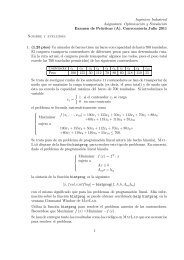
1 INTRODUCTION 3On the other hand, (P α ) has also been solved numerically by using a penalty and regularizationtechnique (see [7]). In this method, the cost function in (P α ) is replaced by12 ‖v‖2 L s (Ω) + 1 2 k ‖y (T )‖2 L 2 (Ω) ,where the penalty parameter k = k(α) is chosen large enough so that ‖y(T )‖ L2 (Ω) ≤ α holds. The use ofthe L s -norm (s large enough) instead of the L ∞ -norm avoids the problem of the non-differentiability ofthe L ∞ -norm and of any power of it. Numerical simulation results within this approach and for the caseof internal point-wise control are described in [7].In this work we propose an alternative approach to solve numerically (P α ). Precisely, we take advantageof the bang-bang structure of the control and hence consider from the very beginning the controlsystem {yt − ∆y + ay = [λ1 O + (−λ)(1 − 1 O )]1 ω , (x, t) ∈ Q T(5)y(σ, t) = 0, (σ, t) ∈ Σ T , y(x, 0) = y 0 (x), x ∈ Ω.Notice that here, we impose a priori that the control v is of bang-bang type, that is, it takes only twovalues, λ on O ∩ q T and −λ on (Q\O) ∩ q T , respectively. λ is the amplitude of the piecewise constantcontrol and O depends on (x, t) but no volume constraint nor regularity assumption are introduced onO. Accordingly, for any α > 0, we consider the optimization problemwhere(BB α ){Minimize in (λ, 1 O ) : 1 2 λ2subject to (λ, 1 O ) ∈ D α (y 0 , T )D α (y 0 , T ) = {(λ, 1 O ) ∈ R + × L ∞ (q T ; {0, 1}) : y = y(λ, O) solves (5) and satisfies ‖y(T )‖ L 2 (Ω) ≤ α}.(7)Thus, (BB α ) can be viewed as an optimal design problem where we design the space-time regionwhere the control takes its two possible values and the optimality is related to the amplitude of thebang-bang control. We would like to emphasize that this formulation makes sense and is of a practicalinterest even if the control of minimal L ∞ -norm is not of bang-bang type. Indeed, we address directlythe problem of computing bang-bang type controls with minimal amplitude which, as indicated above, isof a major interest in practice. Up to our knowledge, this perspective has not been addressed so far.Since the space of admissible designs is not convex, we first obtain a well-posed relaxed formulationand then show how this equivalent but new formulation allows to obtain, for any α > 0 arbitrarily small,a robust approximation of the solution of the original problem. Precisely, in Section 2 we introduce andanalyze this relaxed formulation (see Theorem 2.1). In particular, we obtain that the relaxed problemis an equivalent penalty version of (P α ) and prove that there exists a minimizing sequence of bang-bangtype controls (see Remark 1 and Theorem 2.1, part 3, for precise statements). Then, we derive anddiscuss the first-order necessary optimality condition of the relaxed problem. From this, we recover thebang-bang structure of the control for the pure heat equation and in one space dimension.The case where the control acts on a part of the boundary in Dirichlet and Neumann forms is alsoconsidered and the same type of results are obtained. The numerical resolution of the relaxed problemis addressed in Section 3. We describe the algorithm used to solve the relaxed problem and presentseveral numerical experiments. In particular, the approach allows to capture the oscillatory behavior ofthe control, as α goes to zero.(6)

2 RELAXATION AND NECESSARY OPTIMALITY CONDITIONS 42 Relaxation and necessary optimality conditions2.1 The inner caseWe adopt a penalty approach and for simplicity, we still use α to denote the penalty parameter. Hencewe transform (BB α ) into the following problem:⎧()Minimize in (λ, 1 O ) : J α (λ, 1 O ) = 1 2λ 2 + 1 α ‖y (T )‖2 L 2 (Ω)(T α )⎪⎨⎪⎩subject toy t − ∆y + ay = λ [(2 1 O − 1)] 1 ω , (x, t) ∈ Q T ,y (σ, t) = 0,(σ, t) ∈ Σ Ty (x, 0) = y 0 (x) ,x ∈ Ω(λ, 1 O ) ∈ R + × L ∞ (q T ; {0, 1}) .Accordingly, we also consider the problem⎧()Minimize in (λ, s) : J α (λ, s) = 1 2λ 2 + 1 α ‖y (T )‖2 L 2 (Ω)subject to⎪⎨(RT α )y t − ∆y + ay = [λ (2s (x, t) − 1)] 1 ω ,y (σ, t) = 0,y (x, 0) = y 0 (x)⎪⎩(λ, s) ∈ R + × L ∞ (q T ; [0, 1])(x, t) ∈ Q T(σ, t) ∈ Σ Tx ∈ ΩFrom now on we consider the space L ∞ (q T ; [0, 1]) endowed with the usual weak-⋆ topology. We thenhave the following result.Theorem 2.1 (RT α ) is a true relaxation of (T α ) in the following sense:1. there exists one minimizer of (RT α ) ,2. up to subsequences, every minimizing sequence, say (λ n , 1 On ) of (T α ) converges to some (λ, s) ∈R + × L ∞ (q T ; [0, 1]) such that (λ, s) is a minimizer for (RT α ) , and conversely,3. if (λ, s) is a minimizer for (RT α ) and if 1 On converges to s weak-⋆ in L ∞ (q T ; [0, 1]) , then, up to asubsequence, (λ, 1 On ) is a minimizing sequence for (T α ) .Proof. Let us first prove that the functional J α (λ, s) is continuous. Assume that (λ n , s n ) ∈ R + ×L ∞ (q T ; [0, 1]) satisfies{λn → λs n ⇀ s weak − ⋆ in L ∞ (q T ; [0, 1])as n → ∞.Since [λ n (2s n (x, t) − 1)] ⇀ [λ (2s (x, t) − 1)] weak-⋆ in L ∞ (q T ; [0, 1]) (in particular, also weakly inL 2 (q T )), the solution y n of the system⎧⎨⎩yt n − ∆y n + ay n = [λ n (2s n (x, t) − 1)] 1 ω ,y n (σ, t) = 0,y n (x, 0) = y 0 (x)satisfies { y n ⇀ y weakly in L 2 ( 0, T ; H 1 0 (Ω) )y n t ⇀ y t weakly in L 2 ( 0, T ; H −1 (Ω) ) ,(x, t) ∈ Q T(σ, t) ∈ Σ Tx ∈ Ω

2 RELAXATION AND NECESSARY OPTIMALITY CONDITIONS 5where y = y (x, t) solves⎧⎨⎩y t − ∆y + ay = [λ (2s (x, t) − 1)] 1 ω , (x, t) ∈ Q Ty (σ, t) = 0,(σ, t) ∈ Σ Ty (x, 0) = y 0 (x) x ∈ Ω.By Aubin’s lemma, up to a subsequence still labeled by n,Hence, up to a subsequence,y n → y strongly in L 2 ( 0, T ; L 2 (Ω) ) .y n (t, ·) → y (t, ·) strongly in L 2 (Ω) and a.e. t ∈ [0, T ] . (8)Since y n (t) are continuous functions, convergence (8) in fact holds for all t ∈ [0, T ]. In particular,J α (λ n , s n ) → J α (λ, s) as n → ∞.Moreover, J α (λ, s) is clearly coercitive. As a consequence, problem (RT α ) has a solution.Statements 2. and 3. are a straightforward consequence of the continuity of J α (λ, s) and of thedensity of the space L ∞ (q T ; {0, 1}) in L ∞ (q T ; [0, 1]) .Remark 1 Notice that if we denote by v = λ (2s − 1) (so that λ = ‖v‖ L ∞), then the state law in problem(RT α ) equals the system (1). This way, (RT α ) is the penalty version of (P α ). Moreover, as a consequenceof the continuity of J α we conclude that there exists a minimizing sequence of bang-bang type controls forthe penalty version of the approximate controllability problem (P α ).Next, we analyze the first-order necessary optimality condition for the relaxed problem (RT α ) .Theorem 2.2 The functional J α as defined in problem ) (RT α ) is Gâteaux differentiable and its directionalderivative at (λ, s) in the admissible direction(̂λ, ŝ is given by∂J α (λ, s)∂(λ, s)( ∫) ∫· (ˆλ, ŝ) = ˆλ λ − p(2s − 1) dx dt − 2λ pŝ dxdt (9)q T q Twhere p ∈ C ( [0, T ] ; L 2 (Ω) ) ∩ L 2 ( 0, T ; H 1 0 (Ω) ) solves the adjoint equationProof.{− pt − ∆p + ap = 0, (x, t) ∈ Q Tp(σ, t) = 0, (σ, t) ∈ Σ T , p(x, T ) + α −1 y(x, T ) = 0, x ∈ Ω.)()Let(̂λ, ŝ ∈ R + ×L ∞ (q T ; [0, 1]) be an admissible direction, i.e., for ε small enough, λ + ε̂λ, s + εŝ ∈R + × L ∞ (q T ; [0, 1]) . Denote by y (λ+ε̂λ,s+εŝ)the solution of the state law as defined in (RT α ) associated()with the perturbation λ + ε̂λ, s + εŝ . Thanks to the linearity of the heat equation it is easy to see thaty (λ+ε̂λ,s+εŝ)= y (λ,s) + εŷ + ε 2 ỹ(10)where y (λ,s) is the state associated with the control (λ, s) , ŷ is a solution to⎧[⎨ ŷ t − ∆ŷ + aŷ = 2 λŝ + ̂λ](s − 1) 1 ω , (x, t) ∈ Q T⎩ŷ (σ, t) = 0 (σ, t) ∈ Σ T , ŷ (x, 0) = 0 x ∈ Ω,(11)

and ỹ solves {ỹt − ∆ỹ + aỹ = ̂λŝ1 ω , (x, t) ∈ Q T2 RELAXATION AND NECESSARY OPTIMALITY CONDITIONS 6A straightforward computation shows that∂J α (λ, s)∂(λ, s)ỹ(σ, t) = 0, (σ, t) ∈ Σ T , ỹ (x, 0) = 0 x ∈ Ω.()J α λ + ε̂λ, s + εŝ· (ˆλ, ŝ) = limε→0 ε− J α (λ, s)= λ̂λ + 1 ∫αΩy (λ,s) (T ) ŷ (T ) dx. (12)On the other hand, taking into account the initial condition ŷ (0) = 0 and the final condition p (T ) =−α −1 y (T ) , from the weak form of the system (11) it is deduced that∫∫∫1y (λ,s) (T ) ŷ (T ) dx = −̂λ (2s − 1) dxdt − 2λ pŝdxdtα Ωq T q Tfor p ∈ W (0, T ) = { v ∈ L ( 2 0, T ; H0 1 (Ω) ) : v t ∈ L ( 2 0, T ; H −1 (Ω) )} solution of (10).expression into (12) we obtain (9).Replacing thisCorollary 2.1 Let (λ ⋆ , s ⋆ ) ∈ R + × L ∞ (q T ; [0, 1]) be an optimal solution of (RT α ). Then s ⋆ takes theform{ 0 if p (x, t) < 0s ⋆ (x, t) =(13)1 if p (x, t) > 0and λ ⋆ = ‖p‖ L 1 (q T ). Consequently, if N = 1 or if the potential a = 0 for N > 1, then s⋆ is a characteristicfunction and therefore problem (T α ) is well-posed, i.e., the control is of bang-bang type.Proof.Let (λ ⋆ , s ⋆ ) ∈ R + × L ∞ (q T ; [0, 1]) be an optimal solution of (RT α ). From (9) it follows that( ∫) ∫(λ − λ ⋆ ) λ ⋆ − p(2s ⋆ − 1) dx dt − 2λ ⋆ p(s − s ⋆ ) dxdt ≥ 0 (14)q T q Tfor all (λ, s) ∈ R + × L ∞ (q T ; [0, 1]) . In particular, if λ = λ ⋆ , then∫∫ps ⋆ dxdt ≥ psdxdt ∀s ∈ L ∞ (q T ; [0, 1]) .q T qAn standard localization argument (see for instance [15, pages 67-69]) shows that this variational inequalityis equivalent to the point-wise variational inequalityp (x, t) s ⋆ (x, t) ≥ p (x, t) s (x, t) ∀s ∈ L ∞ (q T ; [0, 1]) , for a.e. (x, t) ∈ q T .From this we easily obtain (13).Now consider the case of the pure heat equation, i.e., a = 0. Using the fact that thanks to theanalyticity of p the zero set of p has zero Lebesgue measure, we conclude that s ⋆ is a characteristicfunction. The same holds if a ≠ 0 and N = 1 (see [2]).Finally, if we put s = s ⋆ in (14), then∫λ ⋆ = p (2s ⋆ − 1) dxdt = ‖p‖ L1 (q T ) ,q Twhere the last equality is a consequence of (13). Remark that from this last equality and (13), the optimalcontrol λ ⋆ (2s ⋆ − 1) has exactly the structure given by (3).Remark 2 Notice that even in the case where (T α ) is well-posed, the relaxed formulation (RT α ) is notuseless. Indeed, at the numerical level, since the admissibility set for (RT α ) is convex (contrary to whathappens in (T α )), it is allowed to make variations in this space and therefore we may implement adescent algorithm to solve (RT α ), and consequently also (T α ). Moreover, Theorem 2.1, part 3, providesa constructive way of computing a minimizing sequence of bang-bang type controls for the general case ofthe heat equation with a potential in dimension N > 1.

2 RELAXATION AND NECESSARY OPTIMALITY CONDITIONS 72.2 The boundary caseIn this section we address the situation in which the control acts on a part of the boundary. We considerboth the cases of Dirichlet and Neumann type controls.2.2.1 Dirichlet-type controlsFor a fixed α > 0, we focus on the control system⎧⎨ y t − ∆y + ay = 0,y (σ, t) = f (σ, t) 1⎩Σ0y (x, 0) = y 0 (x)(x, t) ∈ Q T(σ, t) ∈ Σ Tx ∈ Ω(15)and look for the control f, with support in Σ 0 = Γ 0 × (0, T ), which satisfies‖y (T )‖ H −1 (Ω)≤ α. (16)It is important to notice that we have moved from the L 2 −norm for the final state to the H −1 −normbecause, as noticed in ([10, p. 217]), if we take f ∈ L 2 (Σ 0 ) and y 0 ∈ L 2 (Ω), then, in general, we do nothave y (T ) ∈ L 2 (Ω) .Under some technical assumptions, some positive results concerning the existence of a solution for theapproximate controllability problem (15)-(16) are obtained in [5].Similarly to the inner situation, we consider the optimization problem⎧()Minimize in (λ, 1 O ) : J α (λ, 1 O ) = 1 2λ 2 + 1 α ‖y (T )‖2 H −1 (Ω)(B α )⎪⎨⎪⎩subject toy t − ∆y + ay = 0,y (σ, t) = λ [2 1 O − 1] 1 Σ0y (x, 0) = y 0 (x) ,(λ, 1 O ) ∈ R + × L ∞ (Σ 0 ; {0, 1})(x, t) ∈ Q T(σ, t) ∈ Σ Tx ∈ Ωwith y 0 ∈ L 2 (Ω) .We also consider the new problem⎧()Minimize in (λ, s) : J α (λ, s) = 1 2λ 2 + 1 α ‖y (T )‖2 H −1 (Ω)subject to⎪⎨(RB α )y t − ∆y + ay = 0,y (σ, t) = λ [2s (σ, t) − 1] 1 Σ0y (x, 0) = y 0 (x) ,⎪⎩(λ, s) ∈ R + × L ∞ (Σ 0 ; [0, 1]) .(x, t) ∈ Q T(σ, t) ∈ Σ Tx ∈ ΩThen, we have:Theorem 2.3 (RB α ) is a relaxation of (B α ) in the same terms as stated in Theorem 2.1.Before proving this result, we recall some results concerning the properties of the solution to thefollowing non-homogeneous system:⎧⎨ y t − ∆y + ay = 0, (x, t) ∈ Q Ty (σ, t) = f (σ, t) (σ, t) ∈ Σ⎩T(17)y (x, 0) = y 0 (x) x ∈ Ω,with f ∈ L ∞ (Σ T ) and y 0 ∈ L 2 (Ω) .

2 RELAXATION AND NECESSARY OPTIMALITY CONDITIONS 8Following [10, pp. 208-221] or [11, Vol. II, p.86], a weak solution of (17) is a function y ∈ L 2 (Q T )which satisfies ∫∫∫y(−ϕ t − ∆ϕ + aϕ)dxdt = y 0 (x)ϕ(x, 0)dx − f∂ ν ϕdΣ TQ T ΩΣ Tfor all ϕ ∈ X 1 (Q T ) = { v ∈ H 2,1 (Q T ) : v = 0 on Σ T and v (x, T ) = 0, x ∈ Ω } . As usual, ∂ ν ϕ denotesthe directional derivative of ϕ in the direction of the outward unit normal vector to Γ. Then, itis proved (see also [5, Prop. 5.1]) that there exists a unique weak solution of system (17) which has theregularity( )y ∈ H 1/2,1/4 (Q T ) = L 2 0, T ; H 1/2 (Ω) ∩ H 1/4 ( 0, T ; L 2 (Ω) ) .Moreover, the estimate‖y‖ H 1/2,1/4 (Q T ) ≤ c (‖f‖ L∞ (Σ T ) + ‖y 0‖ L2 (Ω))holds. In particular,)‖y‖ L2 (0,T ;L 2 (Ω))(‖f‖ ≤ c L∞ (Σ T ) + ‖y 0‖ L 2 (Ω). (18)On the other hand, standard arguments show that the weak solution of (17) also satisfies y t ∈ L ( 2 0, T ; H −2 (Ω) )and)‖y t ‖ L2 (0,T ;H −2 (Ω))(‖f‖ ≤ c L∞ (Σ T ) + ‖y 0‖ L2 (Ω). (19)Finally, we also notice that y ∈ C ( [0, T ] ; H −1 (Ω) ) , see [11, Vol. I, Th. 3.1]. As a consequence, the costfunctionals J α and J α above are well-defined.Proof of Theorem 2.3. The proof follows the same lines as in Theorem 2.1 so that we only indicate themain differences. To prove the continuity of J α , let us take (λ n , s n ) ∈ R + × L ∞ (Σ 0 ; [0, 1]) such that{λn → λs n ⇀ s weak − ⋆ in L ∞ (Σ 0 ; [0, 1]) .From estimates (18) and (19) it follows that the corresponding weak solution of⎧⎨ yt n − ∆y n + ay n = 0,(x, t) ∈ Q Ty⎩n (σ, t) = λ n (2s n (σ, t) − 1) 1 Σ0 (σ, t) ∈ Σ Ty n (x, 0) = y 0 (x) x ∈ Ω,satisfies { y n ⇀ y weakly in L 2 ( 0, T ; L 2 (Ω) )where y = y (x, t) solves⎧⎨⎩y n t ⇀ y t weakly in L 2 ( 0, T ; H −2 (Ω) ) ,y t − ∆y + ay = 0,(x, t) ∈ Q Ty (σ, t) = λ (2s (σ, t) − 1) 1 Σ0 (σ, t) ∈ Σ Ty (x, 0) = y 0 (x) x ∈ Ω.Again by Aubin’s lemma, up to a subsequencey n → y strongly in L 2 ( 0, T ; H −1 (Ω) ) .Hence, as in the inner case, we haveJ α (λ n , s n ) → J α (λ, s) as n → ∞.The rest of the proof runs as in Theorem 2.1.

2 RELAXATION AND NECESSARY OPTIMALITY CONDITIONS 9Remark 3 We notice that if the initial condition y 0 ∈ L ∞ (Ω) , then the solution of system (17) satisfiesy ∈ L ∞ (Q T ) (see [10, p.221]). In particular, y (T ) ∈ L 2 (Ω) and therefore the H −1 (Ω) −norm in thecosts J α and J α may be replaced by the L 2 (Ω) −norm.From now on, we assume that y 0 belongs to L ∞ (Ω) and then replace in J α and J α the termα −1 ‖y(T )‖ 2 H −1 (Ω) by α−1 ‖y(T )‖ 2 L 2 (Ω). Similarly to Theorem 2.2 and Corollary 2.1 we have:Theorem 2.4 For y 0 ∈ L ∞ (Ω) the functional J α as defined)above is Gâteaux differentiable and itsdirectional derivative at (λ, s) in the admissible direction(̂λ, ŝ is given by∂J α (λ, s)∂(λ, s)where p solves the backward equation (10).() ∫· (ˆλ, ŝ) = ˆλ λ + ∂ ν p(2s − 1) dΣ 0 + 2λ ∂ ν pŝ dΣ 0 (20)∫Σ 0 Σ 0Corollary 2.2 Let (λ ⋆ , s ⋆ ) ∈ R + × L ∞ (Σ 0 ; [0, 1]) be an optimal solution of (RB α ). Then s ⋆ takes theform{ 0 ifs ⋆ ∂ν p (σ, t) < 0(σ, t) =(21)1 if ∂ ν p (σ, t) > 0and λ ⋆ = ‖∂ ν p‖ L 1 (Σ 0).As a consequence, if N = 1 or if the potential a = 0 for N > 1, then s ⋆ is acharacteristic function and therefore problem (B α ) is well-posed, i.e., the control is of bang-bang type.2.2.2 Neumann-type controlsConsider the system⎧⎨⎩y t − ∆y + ay = 0 in Q T∂ ν y = g on Σ Ty (0) = y 0 in Ω.It is well-known (see for instance [11] or [15]) that for y 0 ∈ L 2 (Ω) and g ∈ L ( 2 0, T ; H −1/2 (Γ) ) thesystem (22) has a unique solution y ∈ L ( 2 0, T ; H 1 (Ω) ) ∩ C ( [0, T ] ; L 2 (Ω) ) which satisfies the variationalformulation∫∫dy (x, t) v (x) dx + [∇y (x, t) ∇v (x) + a (x, t) y (x, t) v (x)] dx = < g (t) , v > Γ ∀v ∈ H 1 (Ω) ,dtΩΩwhere < ·, · > Γ stands for the duality product in H 1/2 (Γ) . Moreover,()‖y‖ C([0,T ];L 2 (Ω)) + ‖y‖ L 2 (0,T ;H 1 (Ω)) ≤ C ‖y 0 ‖ L 2 (Ω) + ‖g‖ L 2 (0,T ;H −1/2 (Γ)).andWith the same notation as in the preceding section, we consider the two problems⎧()Minimize in (λ, 1 O ) : J α (λ, 1 O ) = 1 2λ 2 + 1 α ‖y (T )‖2 L 2 (Ω)(NB α )(RNB α )⎪⎨⎪⎩⎧⎪⎨⎪⎩subject toMinimize in (λ, s) : J α (λ, 1 O ) = 1 2subject toy t − ∆y + ay = 0 in Q T∂ ν y (σ, t) = λ [21 O (σ, t) − 1] 1 Σ0 on Σ Ty (0) = y 0 in Ω(λ, 1 O ) ∈ R + × L ∞ (Σ T ; {0, 1})()λ 2 + 1 α ‖y (T )‖2 L 2 (Ω)y t − ∆y + ay = 0 in Q T∂ ν y (σ, t) = λ [2s (σ, t) − 1] 1 Σ0 on Σ Ty (0) = y 0 in Ω(λ, s) ∈ R + × L ∞ (Σ T ; [0, 1]) .(22)

3 ALGORITHM - NUMERICAL EXPERIMENTS 10The same type of arguments as the ones used in the two preceding cases lets prove that (RNB α ) is arelaxation of (NB α ). Also, a direct computation shows that the functional ) J α is Gâteaux differentiableand its directional derivative at (λ, s) in the admissible direction(̂λ, ŝ is given by∂J α (λ, s)∂ (λ, s)where p solves the system) () ∫·(̂λ, ŝ = ̂λ λ + p (2s − 1) dΣ 0 + 2λ ŝpdΣ, (23)∫Σ 0 Σ 0⎧⎨⎩−p t − ∆p + ap = 0 in Q T∂ ν p = 0 on Σ T(24)p (T ) = 1 α y (T ) in Ω.By using (23), it is not hard to show that if (λ ⋆ , s ⋆ ) is a solution of (RNB α ), then{ 0 if p (σ, t) > 0s ⋆ (σ, t) =1 if p (σ, t) < 0and λ ⋆ = ‖p‖ L 1 (Σ 0)3 Algorithm - Numerical experiments3.1 Algorithm and numerical approximationLet us provide some details on the inner situation and in the one dimensional space case. From now on,we take Ω = (0, 1).First notice that we may remove the constraint λ ∈ R + since, if (λ, s) solves (RT α ), then (−λ, 1 − s)is also a solution. Hence, the expression (9) provides the following iterative descent algorithm :⎧(λ 0 , s 0 ) ∈ R × L ∞ (Q T , [0, 1]),⎪⎨∫)λ n+1 = λ n − a n(λ n − p n (2s n − 1) dx dt , n ≥ 0,(25)q T⎪⎩s n+1 = P [0,1] (s n + b n λ n p n ), n ≥ 0where p n solves (10), P [0,1] (x) = max(0, min(1, x)) denotes the projection of any x onto [0, 1] and a n , b ndenote the optimal descent step which is obtained as the solution of the extremal problem :min J α (λ n+1 (a), s n+1 (b)) over a, b ∈ R + . (26)Problem (26) is solved by using line search techniques. The gradient algorithm is stopped as soon as∫|λ n − p n (2s n − 1)dxdt| ≤ σ (27)q Tfor some given tolerance σ > 0 small enough. In the sequel, σ := 10 −3 .As for the numerical discretization, we use the two-step Gear scheme (of second order) for the timeintegration coupled with a P 1 finite element approach for the spatial approximation. Precisely, for largeinteger N x , we consider the N x points x i ∈ [0, 1] such that x 1 = 0, x i < x i+1 and x Nx = 1. We notefor i ∈ {1, N x − 1}, ∆x i = x i+1 − x i and ∆x = max ∆x i . We note by P ∆x the corresponding partitionof Ω = [0, 1] and by P ∆t the corresponding partition of [0, T ], obtained in the same way. Finally, seth = (∆x, ∆x) and Q h the quadrangulation of Q T associated to h so that in particular Q T = ⋃ K∈Q hK.The following (conformal) finite element approximation of L 2 (0, T ; H0 1 (0, 1)) is introduced:X 0h = { ϕ h ∈ C 0 (Q T ) : ϕ h | K ∈ (P 1,x ⊗ P 1,t )(K) ∀K ∈ Q h , ϕ h (0, t) = ϕ h (1, t) = 0 ∀t ∈ (0, T ) }.

3 ALGORITHM - NUMERICAL EXPERIMENTS 11Here P m,ξ denotes the space of polynomial functions of order m in the variable ξ. Accordingly, thefunctions in X 0h reduce on each quadrangle K ∈ Q h to a linear polynomial in both x and t. The spaceX 0h , conformal approximation of L 2 (Q T ) is a finite-dimensional subspace of L 2 (0, T ; H 1 0 (0, 1)). Moreover,the functions ϕ h ∈ X 0h are uniquely determined by their values at the nodes (x i , t j ) of Q h such that0 < x i < 1.Let us now introduce other finite dimensional spaces. First, we setΦ ∆x = { z ∈ C 0 ([0, 1]) : z| k ∈ P 1,x (k) ∀k ∈ P ∆x }.Then, Φ ∆x is a finite dimensional subspace of L 2 (0, 1) and the functions in Φ ∆x are uniquely determinedby their values at the nodes of P ∆x .Secondly, since the variable λ(2s−1) ∈ L ∞ (Q T ) appears in the right hand side of the forward problemin y, it is natural to approximate λ(2s − 1) ∈ L ∞ (Q T ) by a piecewise constant function. Thus, let M hbe the space defined byM h = { µ h ∈ L ∞ (Q T ) : µ h | K ∈ (P 0,x ⊗ P 0,t )(K) ∀K ∈ Q h }.M h is a finite dimensional subspace of L ∞ (Q T ) and the functions in M h are uniquely determined by their(constant) values on the quadrangles K ∈ Q h .Therefore, for any s h ∈ M h and any λ h ∈ R, the approximation y h ∈ X 0h of the solution of (RT α ) isgiven as follows :(i) Consider the times t j = j∆t and set y h | t=0 = π ∆x (y 0 ) ∈ Φ ∆x .(ii) Then, y h | t=t1 is the solution to the linear problem⎧ ∫ 110 ∆t (Ψ − y h| t=0 )z dx + 1 ∫ 1(Ψ x z x + π ∆x A(x, t 1 )Ψz) dx2 0⎪⎨+ 1 ∫ 1((y h | t=0 ) x z x + π ∆x A(x, t Nt )y h | t=0 z) dx2⎪⎩= 1 2 λ h0∫ 10((2s h (x, t 1 ) − 1) + (2s h (x, t 0 ) − 1)z(x) dx ∀z ∈ Φ ∆x , Ψ ∈ Φ ∆x .(iii) Finally, for given n = 1, . . . , N − 1, Ψ ⋆ = y h | t=tn−1 and Ψ = y h | t=tn , y h | t=tn+1 is the solution to thelinear problem⎧ ∫ 1⎪ 1 ⎨2∆t (3Ψ − 4Ψ + Ψ⋆ )z dx +⎪ ⎩0=∫ 10∫ 10(Ψ x z x + π ∆x (A(x, t n−1 ))Ψz) dxµ h (x, t n−1 )z(x) dx ∀z ∈ Φ ∆x , Ψ ∈ Φ ∆x .Here, π ∆x denotes the projection over Φ ∆x .We are thus using the two-step implicit Gear algorithm as a numerical tool to solve numerically theproblem (RT α ). As advocated in [4], where the influence of the time discretization is highlighted, ithas been observed that this second order scheme ensures a better behavior of the underlying gradientalgorithm than, for instance, the implicit Euler scheme. At the finite dimensional level, algorithm (25)reads as follows :⎧(λ 0 h, s 0 h) ∈ R × M h ,⎪⎨∫)λ n+1h= λ n h − a nh(λ n h − p n h(2s n h − 1) dx dt , n ≥ 0,(28)q T⎪⎩s n+1h= P [0,1] (s n h + b nh λ n hp n h), n ≥ 0where p n h is an approximation of the backward problem (10), obtained by using P 1 finite element in spaceand the Gear scheme for the time integration, as described above.

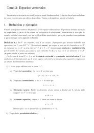
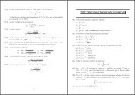
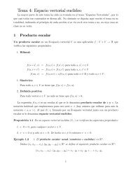
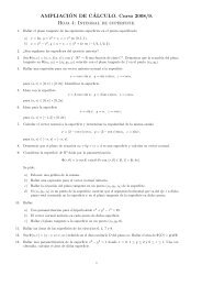
3 ALGORITHM - NUMERICAL EXPERIMENTS 123.2 Numerical experiments3.2.1 Distributed caseWe now provide some numerical results in the one dimensional space case and discuss mainly the influenceof the penalty parameter α. We take Ω = (0, 1) and first consider the data ω = (0.25, 0.75), a ≡ 0 andy 0 (x) = sin(2πx). In order to have a better control of the diffusion, we also replace the operator −∆ by−c∆ with c lower than one. This does not modify the theoretical part.The descent algorithm is initialized with λ = 1 and s = 1/2 over Q T . We take σ := 10 −3 as stoppingcriterion parameter.We take a uniform partition P ∆x for Ω : x i+1 − x i = 1/N x with N x = 400. On the other hand, inorder to describe correctly the oscillations of the density near T , we take a non uniform partition P ∆t ofthe time interval (0, T ): precisely we definet 1 = 0; t j+1 − t j =T pTe pT (eN t− 1− 1)e p(N t +1−j)N T tj = 1, ..., N twhere N t ∈ N is the number of sub-interval of the partition P ∆t and any p ∈ N. The points t j , distributedalong (0, T ), are thus exponentially concentrated near T . This property is amplified for increasing valuesof p. Here p := 6 and N t = 400.Table 1 collects the value of λ h and ‖y h (·, T )‖ L 2 (0,1) with respect to the penalty parameter α. Wetake c := 1/10.We check that the L ∞ -norm λ h of the control increases as α goes to zero : in other words, the amountof work needed to get closer to the zero target at time T is more important. However, as a consequenceof the null controllability of (1) with v ∈ L ∞ (q T ), we check that λ h is uniformly bounded by above withrespect to α.The value α also affects the shape of the bang-bang control. Figure 1 depicts the iso-values of theoptimal density for α = 10 −2 , 10 −4 , 10 −6 and α = 10 −8 . According to the symmetry of ω and of theinitial datum y 0 , we obtain symmetric density over Q T . For α = 10 −2 , the density is constant in timeand related to the sign of y 0 : precisely, for all t, s h (x, t) = 0 if y 0 (x) > 0 and s h (x, t) = 1 if y 0 (x) < 0.However, for α small enough, for instance here, α = 10 −3 , the optimal density exhibits some variationswith respect to the variable t. These variations are mainly located at the end of the time interval.Moreover, as α decreases, the number of theses oscillations, that is, the number of theses changes of signof v h increases so that, at the null controllability limit (α = 0) one may expected an oscillatory behaviorof the bang-bang control both in space and time, in an arbitrarily close neighborhood of (0, 1) × {T }.This is in agreement with our observations in the L 2 case (see [14]). Of course, as in the L 2 -case, thisbehavior may only be captured with an arbitrarily finer mesh. The increasing number of iterates neededto satisfy the criterion (27) as α decreases is also a consequence of these oscillations near T .In Figure 1 we also observe that (except for α = 10 −2 ) the optimal density s h is not strictly a bivalued0 − 1 (as it should be almost everywhere) and takes some intermediate values: this is only dueto the numerical approximation and to the very low variation of the cost function with respect to thedensity near the minimum (a bi-valued density is obtained after a very large number of iterates). Figure2 displays the sign of the adjoint solution p (see 10) in q T and also clearly exhibits the variation of thebang-bang control: recall that from (13), s and p are related through the relation 2s − 1 = sign(p).More interesting is the fact that, whatever be the initial value (λ 0 h , s0 h ) ∈ R+ × L ∞ (Q T , [0, 1]) guesswe consider as the starting point for the algorithm, we always get the same limit. This is of course inagreement with the fact the control v of minimal L ∞ -norm is unique, and so the couple (λ, s) defined byv = λ(2s − 1)1 ω is.We now consider both a bounded but discontinuous potential a and a discontinuous initial datum.Precisely, for Ω = (0, 1) and ω = (0.2, 0.6), we take

3 ALGORITHM - NUMERICAL EXPERIMENTS 13α 10 −1 10 −2 10 −4 10 −6 10 −8‖y h (T )‖ L 2 (Ω) 8.96 × 10 −2 5.34 × 10 −2 6.24 × 10 −3 4.37 × 10 −4 9.17 × 10 −5λ h 0.087 0.471 1.309 1.831 1.948♯ iterates 11 213 561 1032 4501Table 1: N x = N t = 400 - y 0 (x) = sin(2πx) - c = 0.111110.90.90.90.90.80.80.80.80.70.70.70.70.60.60.60.6x0.50.5x0.50.50.40.40.40.40.30.30.30.30.20.20.20.20.10.10.10.100 0.1 0.2 0.3 0.4 0.5t000 0.1 0.2 0.3 0.4 0.5t011110.90.90.90.90.80.80.80.80.70.70.70.70.60.60.60.6x0.50.5x0.50.50.40.40.40.40.30.30.30.30.20.20.20.20.10.10.10.100 0.1 0.2 0.3 0.4 0.5t000 0.1 0.2 0.3 0.4 0.5t0Figure 1: N x = N t = 400 - y 0 (x) = sin(2πx) - ω = (0.25, 0.75) - c = 0.1 - From left to right and from topto button, iso-values of the density function s h in Q T for α = 10 −2 , 10 −4 , 10 −6 and α = 10 −8 .

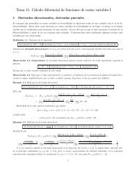
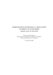
3 ALGORITHM - NUMERICAL EXPERIMENTS 1411110.90.80.90.80.80.60.80.60.70.40.70.40.60.20.60.2x0.50x0.500.40.20.40.20.30.40.30.40.20.60.20.60.10.80.10.800 0.1 0.2 0.3 0.4 0.5t100 0.1 0.2 0.3 0.4 0.5t1Figure 2: N x = N t = 400 - y 0 (x) = sin(2πx) - ω = (0.25, 0.75) - c = 0.1 - Sign of the adjoint state p forα = 10 −6 (left) and α = 10 −8 (right).a (x) ={ 1, 0 ≤ x ≤ 0.5{ 0, x ∈ [0, 0.1] ∪ [0.9, 1]−3, 0.5 < x ≤ 1 , y 0 (x) =1., 0.1 < x < 0.9.(29)The over data remain unchanged. For α = 10 −6 , Figure 3 depicts the iso-values of the optimaldensity s h together with the sign of the corresponding adjoint solution p over Q T . The convergence leadsto λ h ≈ 14.35 for which ‖y h (T )‖ L 2 (0,1) ≈ 4.11 × 10 −6 . Here, of course, the symmetry of the density islost. As in the preceding test, we observe variations of the density near T , up to the error due to thenumerical approximation.11110.90.90.90.80.80.80.80.60.70.70.70.40.60.60.60.2x0.50.5x0.500.40.40.40.20.30.30.30.40.20.20.20.60.10.10.10.800 0.1 0.2 0.3 0.4 0.5t000 0.1 0.2 0.3 0.4 0.5t1Figure 3: Nx = 400 - N t = 400 - ω = (0.2, 0.6) - α = 10 −6 - Discontinuous data as in (29)- Iso-values ofthe density function s h in Q T (left) and sign of p (right).

3 ALGORITHM - NUMERICAL EXPERIMENTS 153.2.2 Boundary caseIn the boundary situation, the density s is simply a time function. This allows to observe clearer thehigh singular character of the bang-bang control as α goes to zero, that is, when one wants to recoverthe null control of minimal L ∞ -norm. The procedure is very similar, except that we also consider a nonuniform partition P ∆x (concentrated on x = 1) in order to better describe the final state p(T ) of theadjoint system (oscillating near x = 1).x 1 = 0; x i+1 − x i = 1e p − 1 (e pNx − 1)e p(Nx+1−i)Nx i = 1, ..., N x .with here p := 3 and still N x = 400.The minimization procedure is similar. For the Dirichlet boundary control considered in Section 2.2.1,fromTheorem 2.4, we may consider the following descent algorithm.⎧(λ 0 h, s 0 h) ∈ R × N h ,⎪⎨λ n+1h= λ n h − a nh(λ n h +⎪⎩∫Σ 0∂ ν p n h(2s n h − 1) dΣ 0), n ≥ 0,s n+1h= P [0,1] (s n h − b nh λ n h∂ ν p n h(1, ·)), n ≥ 0where p n h is as above an approximation of the backward problem (10) and N h the space defined byN h = { µ h ∈ L ∞ ([0, T ]) : µ h | k ∈ P 0,t )(K) ∀k ∈ P ∆t }.As in the inner situation, the residue∫∣ ∣∣∣∣ λn h + ∂ ν p n h(2s n h − 1) dΣ 0Σ 0is used as stopping criterion for the algorithm. For the Neumann boundary control discussed in Section2.2.2, the algorithm is given by⎧(λ 0 h, s 0 h) ∈ R × N h ,⎪⎨λ n+1h= λ n h − a nh(λ n h +⎪⎩∫Σ 0p n h(2s n h − 1) dΣ 0), n ≥ 0,s n+1h= P [0,1] (s n h + b nh λ n hp n h(1, ·)), n ≥ 0(30)(31)where p n his an approximation of the solution p of (24).Let us discuss the Neumann boundary case. We take y 0 (x) = sin(πx), T = 1/2, c = 1/10, a := 0.The stopping criterion is related to the absolute value |λ − ∫ 1p(1, t) (2s − 1) dt|. We stop the algorithm0as soon as this value is lower than 10 −3 . Table 2 reports the L ∞ -norm λ h and the L 2 (0, 1)-norm of y h (T )for various values of the penalty parameter α. The amplitude λ h of the bang-bang control increases asα → 0, and is significantly bigger than in the inner case. This is due to the fact that the control actsonly on a single point of Ω.α 10 −2 10 −4 10 −6 10 −8‖y h (·, T )‖ L2 (Ω) 2.96 × 10 −1 1.59 × 10 −1 5.56 × 10 −2 9.31 × 10 −3λ h 1.488 10.181 29.121 34.03♯ iterates 33 512 6944 20122Table 2: (λ h , y h (T )) with respect to α in the Neumann boundary case.

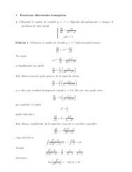
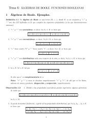
3 ALGORITHM - NUMERICAL EXPERIMENTS 16Figure 4 depicts the optimal density s h with respect to the time variable. We observe here that thedensity is almost everywhere a characteristic function with an increasing number of change of sign as tgoes to T − . Figure 5 depicts the trace, both in time and space, of the approximate controlled solutiony h while Figure 6 displays y h along Q T .Let us insist again on that oscillatory behavior and display the density for α = 10 −6 . Figures 7, 8and 9 depict the optimal density s h (t) for t ∈ [0., 0.5], t ∈ [0.4, 0.5] and t ∈ [0.48, 0.5] respectively. Thesefigures indicates that the frequency of these sign changes increases as t is close to T . Moreover, thenumber of these sign’ changes increases as α → 0. In spite of this singular phenomenon, we observe againthe invariance of the limit (λ h , s h ) of the algorithm with respect to the initialization, consequence of theuniqueness of the minimal L ∞ - norm control.At the limit in α → 0, we expect a bounded amplitude λ h but an arbitrarily large number of oscillationsnear T , in full agreement with our observations for the L 2 situation in [14]. The figures also confirm,in agreement with the optimality conditions for J α that, the optimal density is almost everywhere acharacteristic function, so that no relaxation is needed. The only point where the density is not 0 or 1 isat the final time: From Figure 9, s h (T ) is close to 1/2, intermediate value which reinforces the property,that at the limit in α, the null control highly oscillates at t = T − .110.80.80.60.60.40.40.20.2000 0.1 0.2 0.3 0.4 0.5t0.38 0.4 0.42 0.44 0.46 0.48 0.5tFigure 4: Neumann case - The optimal density s h (t) for t ∈ [0, T ] - α = 10 −4 .For Dirichlet boundary control, the situation is very similar: we simply report here in Table 3 theoptimal couple (λ h , ‖y h (T )‖ L2 (0,1)) with respect to α.α 10 −2 10 −4 10 −6 10 −8‖y h (·, T )‖ L 2 (Ω) 9.21 × 10 −2 3.28 × 10 −3 7.31 × 10 −4 2.34 × 10 −5λ h 0.98 5.12 7.30 9.02♯ iterates 21 319 4912 9301Table 3: (λ h , ‖y h (T )‖ L2 (0,1)) with respect to α in the Dirichlet boundary case.

3 ALGORITHM - NUMERICAL EXPERIMENTS 171050510150 0.1 0.2 0.3 0.4 0.5t0.30.250.20.150.10.0500.050.10 0.2 0.4 0.6 0.8 1xFigure 5: Neumann case - Left : y h (1, t) for t ∈ (0, T ) ; Right: y h (x, T ) for x ∈ (0, 1) - α = 10 −4 .Figure 6: Neumann case - Approximated controlled solution y h over Q T

3 ALGORITHM - NUMERICAL EXPERIMENTS 1810.80.60.40.200 0.1 0.2 0.3 0.4 0.5Figure 7: Neumann case - The optimal density s h (t) for t ∈ [0, T ] - α = 10 −6 .t10.80.60.40.200.4 0.42 0.44 0.46 0.48 0.5Figure 8: Neumann case - The optimal density s h (t) for t ∈ [0.4, 0.5] - α = 10 −6 .t

4 CONCLUSION AND FINAL REMARKS 1910.80.60.40.200.48 0.485 0.49 0.495 0.5Figure 9: Neumann case - The optimal density s h (t) for t ∈ [0.48, 0.5] for α = 10 −6 .t4 Conclusion and final remarksThe reformulation of the L ∞ -controllability problem in terms of an optimal design one allows to get awell-posed relaxed formulation and then a simple minimization procedure. In spite of the well-posednessof this formulation, these bang-bang controls highly oscillate near the final time. While the amplitudeof approximate controls is bounded by above with respect to the penalty parameter α, one may suspectthat the number of these oscillations is not. This feature, closely related to the heat kernel regularizationproperty, renders severally ill-posed the numerical approximation of the null control of L ∞ norm. Otherprocedures may be adopted, for instance taking into account the fact that the relaxed cost is quadraticwith respect to the amplitude λ; however, they all share high degree of ill-posedeness. In that respect, theminimization of the relaxed cost is not easier than the minimization of the conjugate function (derivedfrom duality arguments) commonly used. The subtle difference, strongly enhanced for small values of α,comes from the fact that the density s belongs to L ∞ while the dual variable degenerates in an abstractspace.On the other hand, it is also natural to consider the problem of finding the best location of the supportof the control of minimal L ∞ -norm. This problem has been recently addressed by the authors in theL 2 -case (see [13]).Finally, let us mention the wave type equation where the situation is different: in that case, existenceof bang-bang control does not hold in general, as it depends on the initial data (see [8]). This means that,by applying the same procedure, some data may exhibit relaxation, that is, an optimal density takingvalues in (0,1).References[1] G. Alessandrini and L. Escauriaza, Null-controllability of one-dimensional parabolic equations,ESAIM Control Optim. Calc. Var. 14 (2008), no. 2, 284–293.

REFERENCES 20[2] S. Angenent, The zero set of a solution of a parabolic equation, J. reine angew. Math. 390 (1988),79–96.[3] F. Ben Belgacem and S.M. Kaber, On the Dirichlet boundary controllability of the 1-D heat equation:semi-analytical calculations and ill-posedness degre, Inverse Problems 27 (2011), no. 5.[4] C. Carthel, R. Glowinski and J.-L. Lions, On exact and approximate Boundary Controllabilities forthe heat equation: A numerical approach, J. Optimization, Theory and Applications 82(3), (1994)429–484.[5] C. Fabre, J.-P. Puel and E. Zuazua, Approximate controllability of the semilinear heat equation,Proc. Roy. Soc. Edinburgh Sect. A 125 (1995), no. 1, 31–61.[6] A.V. Fursikov and O. Yu. Imanuvilov, Controllability of Evolution Equations, Lecture Notes Series,number 34. Seoul National University, Korea,(1996) 1–163.[7] R. Glowinski, J-L. Lions and J. He, Exact and approximate controllability for distributed parametersystems. A numerical approach. Encyclopedia of Mathematics and its Applications, 117. CambridgeUniversity Press, Cambridge, 2008.[8] M. Gugat and G. Leugering, L ∞ -norm minimal control of the wave equation: on the weakness ofthe bang-bang principle, ESAIM: COCV 14 (2008) 254-283.[9] G. Lebeau and L. Robbiano, Contrôle exact de l’équation de la chaleur, Comm. Partial DifferentialEquations 20 (1995), no. 1–2,[10] J. L. Lions, Contrôle optimal des systèmes gouvernés par des équations aux dérivés partielles, Dunod,collection E.M., 1968.[11] J. L. Lions and E. Magenes, Problèmes aux limites non homogènes et applications. Vol. I and II,Dunod, 1968.[12] S. Micu and E. Zuazua, Regularity issues for the null-controllability of the linear 1-d heat equation.C. R. Acad. Sci. Paris, Ser. I 349 (2011) 673-677.[13] A. Münch and F. Periago, Optimal distribution of the internal null control for the one-dimensionalheat equation, J. Diff. Eq. 250 (2011) 95-111.[14] A. Münch and E. Zuazua, Numerical approximation of null controls for the heat equation: Illposednessand remedies, Inverse Problems 26(8) 2010.[15] F. Tröltzsch, Optimal Control of Partial Differential Equations. Theory, Methods and Applications,Graduate Studies in Mathematics, Vol. 112, AMS, 2010.[16] E. Zuazua, Controllability and observability of partial differential equations: some results and openproblems, In Handbook of Differential Equations: Evolutionary Differential Equation, vol 3, C.M.Dafermos and E. Feireisl eds, Elsevier Science, 527–621 (2006).