Image Restoration with Discrete Constrained Total Variation Part II ...

J Math Imaging Vis 26: 277–291, 2006c○ 2006 Springer Science + Business Media, LLC. Manufactured in The Netherlands.DOI: 10.1007/s10851-006-0644-3Image Restoration with Discrete Constrained Total Variation Part II:Levelable Functions, Convex Priors and Non-Convex CasesJÉRÔME DARBONEPITA Research and Development Laboratory (LRDE), 14-16 rue Voltaire F-94276 Le Kremlin-Bicêtre, France;École Nationale Supérieure des Télécommunications (ENST), 46 rue Barrault, F-75013 Paris, Francejerome.darbon@{lrde.epita.fr, enst.fr}MARC SIGELLEÉcole Nationale Supérieure des Télécommunications (ENST) / LTCI CNRS UMR 5141,46 rue Barrault, F-75013 Paris, Francemarc.sigelle@enst.frPublished online: 30 November 2006Abstract. In Part II of this paper we extend the results obtained in Part I for total variation minimization in imagerestoration towards the following directions: first we investigate the decomposability property of energies on levels,which leads us to introduce the concept of levelable regularization functions (which TV is the paradigm of). Weshow that convex levelable posterior energies can be minimized exactly using the level-independant cut optimizationscheme seen in Part I. Next we extend this graph cut scheme to the case of non-convex levelable energies. We presentconvincing restoration results for images corrupted with impulsive noise. We also provide a minimum-cost basedalgorithm which computes a global minimizer for Markov Random Field with convex priors. Last we show thatnon-levelable models with convex local conditional posterior energies such as the class of generalized Gaussianmodels can be exactly minimized with a generalized coupled Simulated Annealing.Keywords: total variation, level sets, convexity, Markov Random fields, graph cuts, levelable functionsAbbreviations: KAP, Kluwer Academic Publishers; compuscript, Electronically submitted article1. IntroductionTotal variation (TV) is widely used as regularizationterm for image restoration purposes because of its edgepreserving behavior [2, 19–22]. Data fidelity terms areoften convex functions because it leads to convex optimizationproblems. We have dealt with such modelsin Part I of this paper.In Part II of this paper, we extend the theoreticalframework detailed in Part I for computing an exactand fast minimizer of the following problem∫E v (u) =∫f (u(x), v(x)) dx + β g(|∇u|)dx.(1)Data fidelity term f is often a convex functionand typically takes the following L p form:f (u(x),v(x))) =|u(x) − v(x)| p , p ≥ 1. Laplace andGaussian additive noise correspond to the particularcases p = 1 and p = 2, respectively.Concerning the regularization term, the L q form:g(x) =|x| q , q ≥ 1 is of great importance (with TVcorresponding to q = 1), since it is widely used for imagerestoration [18]. This total variation case as well asthe L 1 + TV and L 2 + TV cases were thoroughly investigatedin Part I. Our approach relies on reformulatingthis problem within a discrete framework into independentbinary Markov Random Fields (MRFs) attachedto each level set of an image. Exact minimization is performedthanks to a minimum cost cut algorithm [12].

278 Darbon and SigelleIn this paper we extend these results towards thefollowing directions:First we generalize the decomposability property ofenergies on the level sets, which leads us to introducethe concept of levelable functions. We prove that convexlevelable posterior energies can be minimized exactlyusing the level-independent graph cut optimizationscheme seen in Part I. During the revision of thispaper, we became aware of the work of Zalesky on submodularenergy functions described in [23]. Zaleskystudies the same class of functions as us. He givesconditions on these energies so that they can be exactlyoptimized via a modified submodular functionminimization algorithm [15]. However, no numericalresults are presented.Then we extend this optimization scheme to nonconvexlevelable energies but with convex priors. Inthis case we provide a graph construction such that itsminimum cost cut determines a global minimizer. Noconditions are set on data fidelity terms. Ishikawa [14]solves exactly the same problem using a minimum costcut based approach. The main difference between thetwo methods consists in the different graph structuresobtained. Experiments show both convincing restorationresults for images corrupted with impulse noiseand a quite faster minimum cost cut-based algorithmapplied on our graph than on Ishikawa’s graph. Approacheswhich compute only approximate solutionsare found in [3, 4, 8, 10].Last we show that a large subset of non-levelableconvex posterior energies can be also minimized witha stochastic coupled Simulated Annealing algorithm.This applies for instance to the widely used generalizedGaussian [5] L p + L q models (with p, q ≥ 1).The rest of this paper is organized as follows. InSection 2, we recall the main results obtained in PartI of this paper which will be useful afterwards. Thenin Section 3, we introduce and develop the main propertiesof levelable functions In Section 4 we show thegraph-cut property of non-convex levelable energiesthanks to a nice constrained scheme and we presentsome results. Last in Section 5, we extend all previousschemes to fairly general cases. For sake of clarity, themain demonstrations of theorems have been placed inrelated Appendices at the end of this Part II.2. RecallsIn this section let us recall the main results obtained inPart I that will be used in the sequel of this work. Weassume that u is defined on a finite discrete lattice S andtakes values in the discrete integer set L = [0, L − 1].We denote by u s the value of the image u at the sites ∈ S. An image is decomposed into its level setsusing the decomposition principle [13]. It correspondsto considering all thresholding images u λ where u λ s =1l us ≤λ. Note the original image can be reconstructedfrom its level sets using u s = min{λ, u λ s = 1} as shownin [13]. Recall that we note by s ∼ t the neighboringrelationship between sites s and t, by(s, t) the relatedclique of order two and by N s the local neighborhoodof site s. For simplicity purpose we shall in the sequelwrite sums on cliques of order one and two by ∑ ∑s and(s,t) respectively.Proposition 1. The discrete version of energy (1)rewrites as follows∑L−2E v (u) = E λ (u λ ) + C, where (2)E λ (u λ ) = βλ=0[ ∑(s,t)+ ∑ s(( )w st 1 − 2uλt uλs + u λ ) ]t(g s (λ + 1) − g s (λ)) ( 1 − u λ )sg s (x) = f (x, v s ) ∀s ∈ S and C = ∑ s(3)g s (0).Note that each Ev λ (·) is a binary MRF with an Ising priormodel. We endow the space of binary configurationsby the following order: a ≼ b iff a s ≤ b s ∀s ∈ S. Inorder to minimize E v (·) one would like to minimize allEv λ(·) independently. Thus we get a family {ûλ } whichare respectively minimizers of Ev λ (·). Suppose we doso, then clearly the summation will be minimized andthus we have a minimizer of E v (·) provided this familyis monotone, i.e.,û λ ≼ û μ ⇔ û λ s ≤ ûμ s ∀λ ≤ μ, ∀s ∈ S. (4)If this property holds then the optimal solution is givenby the reconstruction formula from level sets [13]:û s = min{λ, û λ s = 1} ∀s. Else the family {uλ } does notdefine a function, and thus our optimization scheme isno more valid.The following Lemma is absolutely crucial for ourpoint.Lemma 1. If the local conditional posterior energy ateach site s can be written as∑L−2(E v (u s | N s ) = φs (λ) u λ s + χ s(λ) ) , (5)λ=0

Image Restoration with Discrete Constrained Total Variation Part II 279where φ s (λ) is a non-increasing function of λ andχ s (λ) is a function which does not depend on u λ s ,then one can exhibit a “coupled” stochastic algorithmminimizing each total posterior energy Ev λ(uλ )while preserving the monotone condition: ∀s, u λ s isnon-decreasing with λ .This Lemma states that given a binary solution a ⋆ tothe problem E λ v (·), there exists at least one solution ˆbto the problem E μ v (·) such that a⋆ ≼ ˆb ∀λ ≤ μ.We also recall that a one-dimensional discrete functionf defined on ]A, B[ is convex on ]A, B[ iff2 f (x) ≤ f (x − 1) + f (x + 1) ∀x ∈]A, B[, or equivalently,f (x + 1) − f (x)isanon-decreasing functionon [A, B[.The following important equivalence was thenestablished:Lemma 2. The requirements stated by this Lemma areequivalent to these: all conditional energies E v (u s |N s )are convex functions of grey level u s ∈ ]0, L − 1[, forany neighborhood configuration and local observeddata.It is indeed easy to prove thatφ s (λ) = Ev λ (uλs = 1|Nsλ ) (− Eλv uλs = 0|Nsλ )=−(E v (λ + 1|N s ) − E v (λ|N s )). (6)As a consequence Lemma 1 applies for both the modelsconvex data fidelty with TV as prior.3. Levelable Regularization EnergiesIn this section we propose an extension of the decompositionproperty of posterior energies on levels previouslyseen for the TV case in view of minimizationpurposes. To this aim we first introduce the concept oflevelable functions of several variables. Then we showtheir decomposition properties on binary MRFs.3.1. A Deductive Construction of DecomposableEnergiesWe first introduce our concept of levelable functions.Definition 1. A function φ of one or several variablesx, y ... ∈ L is levelable if it can be decomposed asa sum on levels, of functions of its variables level-setindicatrices at current level:∑L−1φ(x, y ...) = ψ(λ, 1l λ

280 Darbon and SigelleSee proof in Appendix B.We now characterize the behavior of cliques of ordertwo potentials under mild conditions (from an imageprocessing point of view).Proposition 5. If a symmetric function of two variablesU(x, y) satisfies both assumptions:A3. U(x, y) is a levelable function of x, y.A4. ∀y ∈ L, U(x, y) attains a minimum at x = y.then the functions F, G and S = (F + G)/2 defined inProposition 4 should be increasing on L ∗ = [0, L −2].The related energy writes in this case:U(x, y) =|S(x) − S(y)|+D(x) + D(y)∑L−2= R(λ) | 1l λ

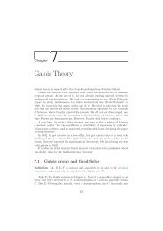
Image Restoration with Discrete Constrained Total Variation Part II 281Figure 1. U(x, y) = F(max(x, y)) − G(min(x, y)) as a function of x (y = 100).Ev λ ( ∣uλ s Nsλ ) I∑=i=1+ ∑ s∑(s,t)τ(s,t)=iR i (λ) ∣ ∣u λ s − uλ ∣tδ(λ, v s ) ( 1 − u λ s). (15)From all what precedes we obtain the followingProposition:Proposition 7. If the total posterior energy E v (u) islevelable and such that all local conditional posteriorenergies E v (·|N s ) are convex functions (even if theirregularization or observation part may not), then thesame level-by-level minimization scheme of Part I appliesfor global optimization.In [23], Zalesky studies the general form of levelablefunction while we have focused on levelable energiesdedicated to image processing. In next section we treatthe minimization of non-convex levelable energies.4. Minimization Algorithms for LevelableEnergiesThe previous level-independent minimization schemecan no more hold for non-convex levelable energies(non-convexity could arise from the attachment to dataas well as from the regularization energies). We arethus led to devise a graph construction such that itsminimum cost cut provides a global minimizer. Wewould to emphasize that Zalesky proposes in [23] a

282 Darbon and Sigelleminimization algorithm which relies on submodularfunction minimization [15], while we propose an algorithmwhich relies on minimum cuts. In the specifictotal variation case we compare our graph structure tothe one proposed by Ishikawa in [14].4.1. Reformulation of the Total Levelable PosteriorEnergyFirst we drop out constant ˜C in Eq. (13) and write thetotal posterior energy as a functional of the (L − 1)binary images u λ :E v ({u λ }) =∑L−2λ=0{ I∑i=1∑(s,t)τ(s,t)=iR i (λ) ∣ ∣u λ s − uλ ∣t4.2. Graph-Cut Representation and MinimizationIn [16], Kolmogorov et al. gives sufficient and necessaryconditions for a fonction to be minimized via graphcuts. Such functions are also called submodular [16].We can now formulate the following proposition:Proposition 8. The unconstrained functionalE α,v ({u λ }) defined by (20) is submodular, i.e.,graph-representable in the sense of Kolmogorovet al. [16].Since each function of a single binary variable is graphrepresentableit is enough to prove the regularity property(defined in [16]):A(0, 0) + A(1, 1) ≤ A(0, 1) + A(1, 0)+ ∑ sδ(λ, v s ) ( 1 − u λ s) } , (16)for each function A(·, ·) of two binary variablesappearing in (20).where R i (·) isapositive non-decreasing function onL. As the convexity assumption no more holds, themonotony condition (4): ∀s ∀λ ≤ μ u λ s ≤ u μ s canthus no more be guaranteed. Since this condition isequivalent to∀s ∀λ ∈ L ∗ u λ s ≤ uλ+1 s , (17)the minimization of (16) is equivalent to the followingconstrained problem:min E v ({u λ }) subject to constraints{u λ }∀s∀λ ∈ L ∗ H ( u λ s − ) uλ+1 s ≤ 0, (18)where H : IR ↦→ IR is the Heaviside function definedasH(x) ={0 if x ≤ 0,1 else.(19)We define for this purpose the new unconstrained energyE α,v ({·λ}) as:E α,v ({u λ }) = E v ({u λ }) + α∑L−2λ=0∑sH ( u λ s − )uλ+1 swith α>0. (20)See proof in Appendix D.We now show in which conditions the minimizationof (20) can lead to a minimizer of (13). We first noticethe following Proposition:Proposition 9. Suppose that {û λ } is a minimizer ofE α,v ({·λ}) such that ∀s ∀λ û λ s ≤ ûλ+1 s . Then the imageû ∈ L S defined as:∀sis a minimizer of E v (·).uˆs = min { λ, u λ s = 1} ,See proof in Appendix E.We now investigate the cases where the hypothesesof Proposition 9 always hold. To this aim we exhibita finite positive value for α such that the monotonyconstraint (17) holds.Proposition 10. Let α > Ɣsup λ,i R i (λ) − inf λ≥1,vsδ(λ, v s ), where Ɣ is the total connectivity. Then a minimizer{û λ } of E α,v ({·λ}) verifies the inequality∀s ∀λ u λ s ≤ uλ+1 s .See proof in Appendix F.The value of α could in fact be adjusted locally foreach site s. Experiments show indeed that α needs notto be so high.

Image Restoration with Discrete Constrained Total Variation Part II 283In other words, we have shown that a levelablefunction with every potential satisfying conditions ofProposition 5 is exactly minimizable via a minimumcost cut. In terms of submodularity, it means that sucha function is a sum of submodular functions over alllevel sets.4.3. Notes on the Graph ConstructionWe now consider the case of the total variation minimization.We briefly compare the approach proposedby Ishikawa [14] which also solves exactly this problemand ours. The Ishikawa’s approach also consistsin building a graph on which a minimum cost cut iscomputed. The structure of this graph is composed oflayers. Each layer corresponds to a grey level. Moreprecisely, a node is created for each value that a pixelcan take. The node n l s which corresponds to the pixelat site s which takes the value l is connected to spatialneighbors at same level, i.e., to nodes n l t with t ∼ s.Itis also connected to nodes n m s with |m − l| =1. Thenodes located at the first (respectively last) layers areconnected to the source (sink respectively). The structureof this graph structurally imposes the monotoneproperty to hold. The Ishikawa’s graph is depicted inFig. 2(a).Contrary to the graph of Ishikiwa, our graph is notmade of layers. However, it contains the same numberof nodes and arcs. A node is created for each binaryvariable u λ s . Each of these nodes is connected to thesource, the sink, the nodes u λ t with s ∼ t, and the nodesu μ s with μ = λ±1. Compared to the graph of Ishikiwa,the main difference is that all nodes are connected tothe source and to the sink. The minimal path from thesource to the sink is equal to 2 for our graph and to Lfor the Ishikiwa’s one. The graph we build is depictedin Fig. 2(b)). A main class of minimum-cut/maximumflow algorithms are based on the augmenting path approach[1]. Such algorithms work iteratively and lookfor a path from the source to the sink where the flow canbe increased. Since our graph is more compact (in thesense that each node is connected to both the source andthe sink) it is reasonable to conjecture that our graphis better suited for augmented path based algorithms.These considerations are confirmed by the numericalexperiments presented in the next section.4.4. Experiments and DiscussionOur implementation relies on the graph constructionproposed by Kolmogorov et al. in [16] and we use thegraph cut algorithm described by Boykov et al. in [7].For all experiments, we have checked that the minimizerscomputed by the Ishikawa’s approach [14] and ouralgorithm have the same energy. We show here our associatedrestoration results when the image is corruptedby impulsive noise of parameter p. The attachment todata term is thus:g s (u s ) = f (u s ,v s )⎧ (⎨− ln (1 − p) + p )=L⎩− ln p else.Lif u s = v s ,This implies that the total energy E v (·) is highly nonconvex.We used a 3 GHz Pentium4 with 1024 KbytesFigure 2. The graph constructed with the Ishikawa approach is depicted in (a) while our graph is presented in (b). We consider a one dimensionalsignal with 3 sites (|S| =3) with 3 available labels (|L| =3). The source and the sink are respectively denoted by s and t. Note that all nodesare connected to the source s and to the sink t for our graph although all arcs are not depicted in b).

284 Darbon and SigelleTable 1. CPU times (in seconds) for total variation minimizationwith an impulsive noise of parameter p and for 256 × 256 sizeimages. The gain factor obtained by our algorithm (Levelable timewrt. Ishikawa time) is also shown.Image Impulsive p Levelable Ishikawa GainLena 0.20 114.78 425.14 3.70Lena 0.40 159.14 633.09 3.98Lena 0.70 252.67 1203.22 4.76Girl 0.20 114.09 469.44 4.11Girl 0.40 171.68 648.72 3.78Girl 0.70 272.72 1553.66 5.70cache memory for our tests. Each experiment has beenrepeated 30 times, using the 4-connectivity approximationof the total variation. Average CPU times for lenaand girl images are given in Table 1 for both our algorithmand Ishikawa’s (image size: 256 × 256). Timeresults show that our graph construction yields a gainfactor about 4 compared to Ishikawa’s method.Associated denoised images for the image girl arepresented in Fig. 3 for noise parameter p with respectivevalues 20%, 40% and 70%. In each of these casesthe regularization parameter β was chosen in order toyield the best visual result. We also observe on Figs.(b) and (d) that minimizers have some pixels which arenot regularized enough. We verify experimentally thatthese pixels do not change during the algorithm. Thisis to compare with observations of Nikolova in [17, 18]for the detection of outliers. In Fig. 4. we compare tothe results from the (sub-optimal) direct random descent.Its principle is the following: pick randomly asite, and a new gray level value. If this new value forthis pixel makes decrease the energy then this transitionis accepted, otherwise the pixel keeps its value. Weiterate this process until no moves are allowed. To concludeat this point, our graph cut method yields verygood results visually speaking, but comparison withother methods such as the morphological approach ofCoupier et al. [9] remains to be done.5. Extension to Convex Non-LevelableRegularization EnergiesIn this section we proceed even further by extendingthe previous results to non-levelable regularization energiesprovided they have a convex form, while no conditionsare imposed on data fidelity terms. As an example,this section shows how to find a global minimizerof energies which has the following form [18]:E v (u)= ∑ j s |u s −v s | p +β ∑ b rs |u s −u t | q p, q ≥1,s∈S(r,s)where j s ≥ 0 is a local “outlier” detector and b rs ≥ 0is a local boundary detector can be exactly minimized.First of all, we present an algorithm based on graph-cutswhich computes an exact minimizer. Note that in [14],Ishikawa solves exactly the same problem with the useof graph-cuts. However, the graphs built are quite differentfrom each others. We also propose an alternativecondition for devising stochastic optimization.5.1. Reformulation of the Total Posterior EnergyOur approach for exact minimization is similar to thatpreviously encountered for the levelable case. Recallthat we assume that priors are convex functions. Moreoverwe shall assume in the sequel that each regularizationpotential (noted U st (u s , u t ) for sake of generality)is also symmetric and depends on the difference of itstwo grey level variables as in Eq. (1), i.e.,U st (u s , u t ) = V st (u s − u t ) = V st (u t − u s ).These assumptions imply the convexity of each V st (·)on ] − L + 1, L − 1[.Now, proceeding similarly to paragraph 4.1 we firstreformulate the total posterior energy as a functionalof the L − 1 binary images u λ .Proposition 11. The total posterior energy (1) can berewritten as:{ ∑L−2∑L−2μ=0 λ=0U λ,μ (st uλs , u μ )tE v ({u λ }) = ∑ (s,t)∑L−2[ ( ) ( )] }+ Dλst uλs + Dλst uλtλ=0+ ∑ sU λ,μ (st uλs , u μ t∑L−2 λ ( ∣ )s uλ ∣v s + C, where (21)λ=0)= Gst (λ, μ) ( 1 − u λ )(μ) s 1 − u t ,with G st (λ, μ) = 2V st (λ − μ) − V st (λ − μ − 1)− V st (λ − μ + 1) ≤ 0,D λ st(uλs)= (Vst (λ + 1) − V st (λ)) ( 1 − u λ s), λ s(uλs |v ) = (g s (λ + 1) − g s (λ)) ( 1 − u λ s),andC = ∑ sg s (0).

Image Restoration with Discrete Constrained Total Variation Part II 285Figure 3. Image girl corrupted with impulse noise. Noise parameter value: (a) : 20%, (c) : 40%, (e) : 70%. Associated respective restorationresults: (b), (d), (f).

286 Darbon and SigelleFigure 4. Results of the restoration of the image girl corrupted with impulse noise using a direct random descent algorithm. Figures (a), (b)and (c) correspond to minimizer of images corrupted with an impulse noise of parameter 20%, 40% and 70%, respectively.The principle relies on decomposing each regularizationpotential as two sums over grey level variablesinstead of one. See Proof in Appendix G.5.2. Graph-Cut Representation and MinimizationThe proposed approach is similar to the one presentedfor levelable energies. We define the constrained totalposterior energy as: E α,v (·)E α,v ({u λ }) = E v ({u λ }) + ∑ s∑L−2αH ( u λ s − )uλ+1 sλ=0with α>0, (22)where H is the Heaviside function defined by Eq. (19).The purpose of this last term is, as before, to enforcethe monotone property Eq. (4) to hold i.e.,∀λ u λ s ≤ uλ+1 s .The fact that regularization terms {V st } are convex functionsis of capital importance for the minimization algorithmthat we present now. Notice that results hold evenfor non-symmetric convex regularization energies.Proposition 12. Let α be a non-negative value. The energyE α,v (·) in Eq. (22) is submodular, i.e., it is graphrepresentablein the Kolmogorov et al. [16] sense.The main argument relies on the fact that each functionof two binary variables in Eq. (21) is graphrepresentablesince all terms G st (λ, μ) ≤ 0 by theconvexity hypothesis. See Proof in Appendix H.We now build a graph associated to E α,v ({·λ}) suchthat its minimum cost cut yields a global minimizer. We

290 Darbon and SigelleH. Proof of Proposition 12Each term of Eq. (22) is submodular, i.e., graphrepresentablein the Kolmogorov et al. [16]:• H : the justification is given in Section 4.• Dst λ and λ s in Eq. (21) are functions of a singlebinary variable. Thus they are graph-representable.• each term U λ,μst (u λ s , uμ t ) = G st (λ, μ)(1−u λ s )(1−uμ t )involving two binary variables in Eq. (21) is graphrepresentablebecause it satisfies the regularity property(see Appendix D Eqs. (23) and (24)):U λ,μst(0, 0) + U λ,μst (1, 1) ≤ U λ,μst (1, 0) + U λ,μst (0, 1),since G st (·, ·) is non-positive by the convexity assumption.In [16], Kolmogorov et al. show that the sum of graphrepresentablefunctions is graph-representable, whichis the case for the energy E α ({·λ}|v). This concludesthe proof.□I. Proof of Proposition 14Each local conditional energy may be decomposed similarlyto Part I as:E v (u s | N s )∑L−2= (E v (λ + 1 | N s ) − E v (λ | N s )) ( 1 − u λ )sλ=0+E v (0 | N s )∑L−2= (φ s (λ) u λ s + χ s(λ))λ=0where φ s (λ) =−(E v (λ + 1 | N s ) − E v (λ | N s )).(28)The local posterior Gibbs distribution at a given levelwrites thus:P ( u λ s = 1 | N ) 1s,v s =1 + exp {φ s (λ)} .Validating the coupled Gibbs sampling scheme of Part Irequires that∀N s ,v s , P ( u λ s = 1|N s,v s)is non-decreasing with λ,and thus from (28):∀N s ,v s , −φ s (λ)= E v (λ+1|N s )−E v (λ|N s ) is non-decreasing with λ.Thus ∀N s ,v s , E v (·| N s ) should be a convex functionon ]0, L − 1[.AcknowledgmentsThe authors would like to thank deeply VincentArsigny (INRIA Sophia EPIDAURE Project), Jean-Francois Aujol (CMLA ENS Cachan) and AntoninChambolle (CMAP Ecole Polytechnique) for enlightingdiscussions.References1. R. Ahuja, T. Magnanti, and J. Orlin, Network Flows: Theory,Algorithms and Applications. Prentice Hall, 1993.2. S. Alliney, “An algorithm for the minimization of mixed l 1 andl 2 norms with application to bayesian estimation,” IEEE Transactionson Signal Processing, Vol. 42, No. 3, pp. 618–627, 1994.3. J. Besag, “On the statistical analysis of dirty pictures,” Journalof the Royal Statistics Society, Vol. 48, pp. 259–302, 1986.4. A. Blake and A. Zisserman, Visual Reconstruction. MIT Press,1987.5. C. Bouman and K. Sauer, “A generalized Gaussian image modelfor edge-preserving MAP estimation,” IEEE Transactions onTransactions on Signal Processing, Vol. 2, No. 3, pp. 296–310,1993.6. S. Boyd and L. Vandenberghe, Convex Optimization. CambridgeUniversity Press, 2004.7. Y. Boykov and V. Kolmogorov, “An experimental comparisonof Min-Cut/Max-Flow algorithms for energy minimization invision,” IEEE Transactions on Pattern Analysis and MachineIntelligence, Vol. 26, No. 9, 1124–1137, 2004.8. Y. Boykov, O. Veksler, and R. Zabih, “Fast approximate energyminimization via graph cuts,” IEEE Transactions on PatternAnalysis and Machine Intelligence, Vol. 23, No. 11, pp. 1222–1239, 2001.9. D. Coupier, A. Desolneux, and B. Ycart, “Image denoising bystatistical area thresholding,” Journal of Mathematical Imagingand Vision, Vol. 22, No. 2–3, pp. 183–197, 2005.10. S. Geman and D. Geman, “Stochastic relaxation, Gibbs distributions,and the bayesian restoration of images,” IEEE PatternAnalysis and Machine Intelligence, Vol. 6, No. 6, pp. 721–741,1984.11. G. Giorgi, A. Guerraggio, and J. Thierfelder, Mathematics ofOptimization: Smooth and Nonsmooth Case. Elsevier Science,2004.12. D. Greig, B. Porteous, and A. Seheult, “Exact maximum a posterioriestimation for binary images,” Journal of the Royal StatisticsSociety, Vol. 51, No. 2, pp. 271–279, 1989.13. F. Guichard and J. Morel, “Mathematical morphology “almosteverywhere,”” in Proceedings of ISMM, 2002, pp. 293–303.14. H. Ishikawa, “Exact optimization for Markov random fields withconvex priors,” IEEE Transactions on Pattern Analysis and MachineIntelligence, Vol. 25, No. 10, pp. 1333–1336, 2003.15. S. Iwata, L. Fleischer, and S. Fujishige, “A combinatorialstrongly polynomial algorithm for minimizing submodular functions,”Journal of the ACM, Vol. 48, No. 4, pp. 761–777,2001.

Image Restoration with Discrete Constrained Total Variation Part II 29116. V. Kolmogorov and R. Zabih, “What energy can be minimizedvia graph cuts?” IEEE Transactions on Pattern Analysis andMachine Intelligence, Vol. 26, No. 2, pp. 147–159, 2004.17. M. Nikolova, “Local strong homogeneity of a regularized extimator,”SIAM Journal on Applied Mathematics, Vol. 61, pp.633–658, 2000.18. M. Nikolova, “A variational approach to remove outliers andimpulse noise,” Journal of Mathematical Imaging and Vision,Vol. 20, pp. 99–120, 2004.19. S. Osher, A. Solé, and L. Vese, “Image decompositionand restoration using total variation minimization and theH −1 norm,” J. Mult. Model. and Simul., Vol. 1, No. 3, 2003.20. I. Pollak, A. Willsky, and Y. Huang, “Nonlinear evolution equationsas fast and exact solvers of estimation problems,” IEEETransactions on Signal Processing, Vol. 53, No. 2, pp. 484–498,2005.21. L. Rudin, S. Osher, and E. Fatemi, “Nonlinear total variationbased noise removal algorithms,” Physica D., Vol. 60, pp. 259–268, 1992.22. K. Sauer and C. Bouman, “Bayesian estimation of transmissiontomograms using segmentation based optimization,” IEEETransactions on Nuclear Science, Vol. 39, No. 4, pp. 1144–1152,1992.23. B. Zalesky, “Efficient determination of Gibbs estimators withsubmodular energy functions,” http://www.citebase.org/cgi-bin/citations?id=oai:arXiv.org:math/0304041, 2003.received the M.Sc. degree in applied mathematics from E.N.S. deCachan, France, in 2001. In 2005, he received the Ph.D. degreefrom Ecole Nationale des Télécommunications (ENST), Paris,France. He is currently a postdoc at the Department of Mathematics,University of California, Los Angeles, hosted by Prof.T.F. Chan. His main research interests include fast algorithmsfor exact energy minimization and mathematical morphology.Marc Sigelle was born in Paris on 18th March 1954. He receivedan engeneer diploma from Ecole Polytechnique Paris 1975 andfrom Ecole Nationale Supérieure des Télécommunications Parisin 1977. In 1993 he received a Ph.D. from Ecole NationaleSupérieure des Télécommunications. He worked first at CentreNational d’Etudes des Télécommunications in Physics andComputer algorithms. Since 1989 he has been working at EcoleNationale Supérieure des Télécommunications in image andmore recently in speech processing. His main subjects of interestsare restoration and segmentation of signals and images withMarkov Random Fields (MRF’s), hyperparameter estimationmethods and relationships with Statistical Physics. His interestsconcerned first reconstruction in angiographic medical imagingand processing of remote sensed satellital and synthetic apertureradar images, then speech and character recognition usingMRF’s and bayesian networks. His most recent interests concerna MRF approach to image restoration with Total Variationand its extensions.Jérôme Darbon was born in Chenôve, France in 1978. From1998 to 2001, he studied computer science at Ecole Pourl’Informatique et les Techniques Avancées (EPITA), France. He