Algorithms for the Weighted Orthogonal Procrustes Problem and ...

UMINF-06.10 ISSN-0348-0542 ISBN 91-7264-052-9

PrefaceThis thesis consists of the following six papers.I. P. Å. Wedin and T. Viklands. Algorithms for 3-dimensional WeightedOrthogonal Procrustes Problems. Technical Report UMINF-06.06, Departmentof Computing Science, Umeå University, Umeå, Sweden, 2006.II. T. Viklands and P. Å. Wedin. Algorithms for Linear Least Squares Problemson the Stiefel manifold. Technical Report UMINF-06.07, Departmentof Computing Science, Umeå University, Umeå, Sweden, 2006.III. T. Viklands. On the Number of Minima to Weighted Orthogonal ProcrustesProblems. Technical Report UMINF-06.08, Department of ComputingScience, Umeå University, Umeå, Sweden, 2006. Submitted forpublication in BIT.IV. T. Viklands. On Global Minimization of Weighted Orthogonal ProcrustesProblems. Technical Report UMINF-06.09, Department of ComputingScience, Umeå University, Umeå, Sweden, 2006. Submitted for publicationin BIT.V. T. Viklands. A Cubic Convergent Iteration Method. Technical ReportUMINF-05.10, Department of Computing Science, Umeå University,Umeå, Sweden, 2005.VI. T. Viklands and M. Gulliksson. Optimization Tools for Solving NonlinearIll-posed Problems. Fast solution of discretized optimization problems(Berlin, 2000), 255–264, Internat. Ser. Numer. Math., 138, Birkhäuser,Basel, 2001.In Chapter 1 an introduction to the optimization problems considered is presentedalong with an overview of all papers. The papers are referred to by theirroman numbers.v

viii

Paper IV 109Paper V 143Paper VI 159Notations 175

Chapter 1Introduction and overviewThe main part of this thesis is about an optimization problem known as theweighted orthogonal Procrustes problem (WOPP), which we define as:Definition 1.0.1 With Q ∈ R m×n where n ≤ m, let A, X and B be knownreal matrices of compatible dimensions with rank(A) = m and rank(X) = n.Let || · || F denote the Frobenius matrix norm. The optimization problemminQ ||AQX − B||2 F , subject to Q T Q = I n , (1.0.1)is called a weighted orthogonal Procrustes problem.The Frobenius matrix norm can be regarded as the Euclidean norm formatrices. For vectors, the Euclidean norm is commonly known as the 2-norm,|| · || 2 . With a vector y ∈ R k , its Euclidean length is∑||y|| 2 = √ k yi 2.i=1For a matrix Y ∈ R m×n , the Frobenius norm ||Y || F ism∑ n∑||Y || F = √ yi,j 2 .i=1 j=1The WOPP is a linear least squares problem defined on a Stiefel manifold.A Stiefel manifold [30], commonly denoted V m,n , is the set of all matrices Q ∈R m×n , having orthonormal columns. V m,n is also referred to as the Stiefelmanifold of orthogonal n-frames in R m ,V m,n = {Q ∈ R m×n : Q T Q = I n }.A set of nonzero vectors {q 1 , ..., q n } in R m is said to be orthogonal if q T i q j =0 when i ≠ j. If additionally q T i q i = 1 (normalized), the set is said to beorthonormal [12].1

2 Chapter 1The definition of an orthogonal matrix is well known. A square matrixQ ∈ R m×m is said to be orthogonal if Q T Q = I m , hence QQ T = I m andQ T = Q −1 . This may seem a bit ambiguous since the columns of Q form notjust an orthogonal basis but also an orthonormal basis. When speaking of anorthonormal matrix Q = [q 1 , ..., q n ], we mean that the columns of Q form anorthonormal basis, i.e., Q T Q = I n . If n = m then Q is orthogonal (a squareorthonormal matrix).Trough out this thesis, we assume that n ≤ m. Evidently Q T Q ≠ I n ifn > m.The WOPP can be regarded as a generalization of the orthogonal Procrustesproblem (OPP).Definition 1.0.2 With Q ∈ R m×n where n ≤ m, let X with rank(X) = nand B be known real matrices of correct dimensions. We call the optimizationproblemmin ||QX −Q B||2 F , subject to Q T Q = I n , (1.0.2)an orthogonal Procrustes problem.The OPP has an analytical solution, that can be derived by using the singularvalue decomposition (SVD) of XB T . The WOPP on the other hand, typicallyneeds to be solved by iterative optimization algorithms.To derive the solution to (1.0.2), use the property that for a matrix Y ∈R m×n , ||Y || 2 F = tr(Y T Y ) where tr(·) is the matrix-trace,We can then writen tr(Ỹ ) = ∑ỹ i,i , Ỹ = Y T Y.i=1||QX − B|| 2 F = tr((QX − B) T (QX − B)) == tr(X T Q T QX) − 2tr(QXB T ) + tr(B T B) = ||X|| 2 F − 2tr(QXB T ) + ||B|| 2 F,since Q T Q = I n . Solving (1.0.2) is then done by maximizing tr(QXB T ). To doso, let UΣV T = XB T be a SVD, thentr(QXB T ) = tr(QUΣV T ) = tr(V T QUΣ) = tr(ΣZ) =n∑σ i,i z i,i (1.0.3)where Z = V T QU. Since Z ∈ R m×n is orthonormal, any z i,j ≤ 1 for alli = 1, . . .,m and j = 1, . . .,n. Hence, the sum in (1.0.3) is maximized ifZ = I m,n , and the solution ˆQ to (1.0.2) is given by ˆQ = V I m,n U T . The OPP iswell studied, and is mentioned in introductory textbooks as, e.g., [12].As a simple and small example of a WOPP, consider the following: Find theminimum distance between the ellipsex = α 1 cosφ , y = α 2 sin φi=1

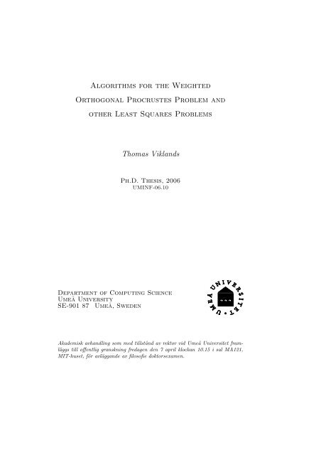
Introduction and overview 3x 2α 2TY ( ˆQ)rBx 1α 1Figure 1: Y (Q) is here an ellipse with semi major and semi minor axes α 1 andα 2 , respectively. The minimum distance occurs at Y ( ˆQ) where the residualr = B − Y ( ˆQ) is orthogonal to the tangent T of Y (Q) at ˆQ.and the point B according to Figure 1.With Q = [cosφ, sin φ] T we can express the ellipse as the vector valuedfunction[ ][ ]α1 0 cosφY (Q) == AQ.0 α 2 sin φFor vectors, the Frobenius norm is the same as the 2-norm. We can write theoptimization problem as a WOPP (with X = 1)minQ ||AQ − B||2 2 , subject to Q T Q = 1. (1.0.4)Since n = 1 in this case, there are no orthogonality constraints. The task is tofind the orthonormal matrix ˆQ (a normalized vector, Q T Q = 1), that minimizesthe distance between the ellipse Y (Q) and the point B. A solution to (1.0.4) canbe computed by using iterative methods as, e.g., Newton’s method. Though, forthis simple case of a WOPP, a solution can also be computed by solving a fourthdegree polynomial, see Paper I. There can also be two different minimizers for(1.0.4), see Section 3.1.Note that if α 1 = α 2 = χ, Y (Q) describes a circle with radii χ. Then bytaking X = χ, (1.0.4) can be written as an OPPminQ ||QX − B||2 2 , subject to QT Q = 1. (1.0.5)The solution ˆQ to (1.0.5) is unique, and is easily computed by taking ˆQ =B/||B|| 2 .

4 Chapter 1Though these examples are very simple, they illustrate the difficulty of computinga solution to a WOPP compared to an OPP.1.1 Procrustes problemsThere are several types of optimization problems involving Stiefel manifolds.One class of problems are different types of Procrustes problems, arising ina wide area of applications. Commonly, the term Procrustes analysis or Procrustesrotation is used instead of Procrustes problems. For example, orthogonalProcrustes analysis and weighted Procrustes rotation to address the OPP andWOPP, respectively.The name Procrustes comes from the Greek mythology. Procrustes (theStretcher) was a robber and torturer that had an iron bed in which he desiredto put his victims. To make them fit the bed he cut of their limbs or alternativelystretched them out. In the end, karma came to Procrustes as he was fitted inhis own bed by Theseus.1.1.1 Rigid body movementsThe ellipse problem discussed is to the least very simple, due to its low dimension(m = 2 and n = 1). To give an example of a WOPP of larger dimension, weconsider the problem of determining a rigid body movement.Consider a rigid body with n landmarks x 1 , ..., x n in R 3 that is subject toa translation t ∈ R 3 , and a rotation M ∈ R 3×3 , taking the landmarks into thepositions c 1 , . . .,c n . In rigid body applications, commonly M (for Motion) isused to represent an orthogonal matrix.x 1Mx i + tx 2x 3c 1c 2c 3Figure 2: A rigid body with three landmarks undergoing a rotation and translation.The motion of the rigid body can be written asMx i + t = b iwhere M, with det(M) = 1, describes the rotations around the three axes.Given x 1 , . . .,x n and c 1 , . . .,c n , the rotation M can be computed by solving an

Introduction and overview 5orthogonal Procrustes problem (OPP) as follows [29]. Let X = [x 1 −¯x, ..., x n −¯x]and C = [c 1 − ¯c, ..., c n − ¯c] where ¯x and ¯c are the mean value vectors of x i andc i , i = 1, ..., n, then M is given by solvingminM ||MX − C||2 F , subject to MT M = I 3 , det(M) = 1. (1.1.1)The solution is given by using the SVD of XC T , and if XC T is nonsingular thesolution is unique.Suppose now that the accuracies of the landmarks x i and x i , i = 1, . . . , n aredifferent, dependent on the coordinate axes (in R 3 ). Let us say, that along thethird axis (z-axis), we have a noticeable lower accuracy than for the first andsecond axes (x- and y-axes). It is then preferred to give these z-axis coordinatesa lesser impact when computing a solution. To do this we can weight the OPPby using a weighting matrix A. For instance, letA =⎡⎣ 1 0 00 1 00 0 αwhere 0 < α < 1 is a suitable chosen scalar. The weighted residual is thenA(MX − C) and we get a WOPP on the formminM ||A(MX − C)||2 F , subject to M T M = I 3 , det(M) = 1. (1.1.2)Observe that by taking B = AC, (1.1.2) is on the form stated in Definition 1.0.1.Commonly iterative optimization algorithms are used to compute a solutionto (1.1.2). Moreover, a WOPP can have several minima, which leads to theproblem of deciding if a computed solution is the ”best” one.It can also be desired to weight the OPP from right. Assume that theaccuracy when measuring some, specific, landmarks is worse than the average.Then by constructing a diagonal matrix W, we can give these landmarks a lowweight as (MX − C)W. The right-weighted OPP then becomesminM ||(MX − C)W ||2 F , subject to M T M = I 3 , det(M) = 1.By taking X := XW and B = CW, we see that solving this problem is doneby solving an OPP.1.1.2 PsychometricsThe OPP originates from factor analysis in psychometrics in the 1950s and1960s, e.g., [16,18]. The task is to determine an orthogonal matrix Q ∈ R m×m ,that rotates a factor (data) matrix A, to fit some hypothesis matrix B. Typicallyin psychometrics, the points to be rotated are ordered row wise in A, not columnwise in X as with the rigid body movement example shown above. We denotethe rotation of A as Y (Q) = AQ. Hence, given A and B, we wish to find Qsuch that Y (Q) ≈ B.⎤⎦ ,

6 Chapter 1When using the Euclidean distance to measure the distance between therotation Y (Q) and B, the optimal orthogonal matrix Q is given by solvingminQ ||AQ − B||2 F , subject to Q T Q = I m . (1.1.3)Since n = m, resulting in that Q is an orthogonal matrix, (1.1.3) is an OPPwith a solution that can be derived by using the SVD of B T A.A more common formulation of the OPP, in psychometrics, is with the usageof the matrix-trace,minQ tr(AQ − B)T (AQ − B) , subject to Q T Q = I m .Extensions of (1.1.3) were later on considered. The case when Q is an orthonormalmatrix, i.e., Q ∈ R m×n with n ≤ m was considered in, e.g., [5]. GivenA and B, it is desired to find Q such that Y (Q) ≈ B but now with Q T Q = I n .In [5], to measure the similarity of the two matrices Y and B, the degree ofcollinearity of the rows yiT and b T i in Y and B respectively is used. Hence, thesolution ˆQ is computed frommax ∑ iy T i b i = max tr(Y B T ) = maxtr(AQB T ) , subject to Q T Q = I n ,(1.1.4)by using the SVD UΣV T = B T A, yielding ˆQ = V I m,n U T . This solution iscomputed in a similar manner as for an OPP. ˆQ is not necessary the same asthe solution given when the Euclidean distance is used, to measure distancesbetween points in Y and B. Then we getminQ ||AQ − B||2 F , subject to QT Q = I n . (1.1.5)By using the matrix-trace, we write the objective function in (1.1.5) as||AQ − B|| 2 F = tr(QT A T AQ) − 2tr(AQB T ) + B T B == tr(AQQ T A T ) − 2tr(AQB T ) + B T B.If n = m, then QQ T = I m and (1.1.5) becomes an OPP whose solution iscomputed by maximizing tr(AQB T ), just as in (1.1.4). The differences occurwhen n < m, since then QQ T ≠ I n , and the term tr(AQQ T A T ) becomesdependent on Q. To illustrate this, we can look at the example in [5]. Therethe hypothetical factor matrices to be matched are,A =⎡⎢⎣0.76 0.32 0.50.5 0.5 −0.40.52 −0.36 0.50.5 −0.5 −0.4⎤ ⎡⎥⎦ , B = ⎢⎣0.7 0.10.8 00.1 0.70 0.8⎤⎥⎦ .

Introduction and overview 7The solution to 1.1.4 is⎡ˆQ = ⎣0.7444 0.66200.6651 −0.74660.0582 0.0657while the solution to (1.1.3) is⎡¯Q = ⎣0.7385 0.65700.6656 −0.7462−0.1073 −0.1076⎤⎦ , Y ( ˆQ) =⎤⎦ , Y ( ¯Q) =⎡⎢⎣⎡⎢⎣0.8077 0.29700.6815 −0.06860.1768 0.64590.0164 0.67800.7206 0.20670.7450 −0.00160.0907 0.55650.0794 0.7446The discrepancies here, for the two different solutions ˆQ and ¯Q, are || ˆQ− ¯Q|| F =0.2398, ||Y ( ˆQ) − B|| F = 0.3052 and ||Y ( ¯Q) − B|| F = 0.2119.It can also be desirable to weight either the columns or the rows in theresidual AQ − B, as described above in the rigid body movement example.When weighting of the columns in AQ − B, we getminQ tr(AQ − B)T ˜W 2 (AQ − B) , subject to Q T Q = I n , (1.1.6)and the weighting of the rows in AQ − B isminQ tr(AQ − B) ¯W 2 (AQ − B) T , subject to Q T Q = I n , (1.1.7)where ˜W and ¯W are known diagonal weighting matrices, [20,22]. If n = m, then(1.1.6) becomes an OPP, in a similar way to the right-weighted OPP in Section1.1.1. Equation (1.1.7) can be written as a WOPP according to Definition 1.0.1,by taking B := B ¯W and X = ¯W.1.1.3 The OPP and WOPPAreas where the WOPP (and OPP) arise are in applications related to, e.g.,rigid body movement and psychometrics as mentioned, factor analysis [15,23],multivariate analysis and multidimensional scaling [6,13], global positioning system[2]. Typically, it is about computing a matrix with orthonormal columns,when it is desired to match one set of data to another.As mentioned earlier, the solution to a WOPP can not be computed aseasily as for an OPP. Additionally, a WOPP can have several local minima.Hence a solution, computed by some iterative method, is not necessarily a globaloptimum. The formulation (1.0.1) has sometimes been referred to as the Penroseregression problem 1 .1 It is not clear from where this originates. It seems as the first time the term ”Penroseregression” was used was in an older version (technical report) of [4] from 1997. Lars Eldéninformed me that Penrose studied the best approximation of the matrix equation AXC = Bwhere A, X, C and B are any general matrices [26].⎤⎥⎦ ,⎤⎥⎦ .

Introduction and overview 91.2 Linear Least squares problems on the StiefelmanifoldIn this thesis, we also consider optimization problems on the form,minQ ||f(Q) − b||2 2 , subject to Q ∈ V m,n , (1.2.1)where f(Q) ∈ R k is a vector valued function of Q and b ∈ R k a known vector.We restrict ourselves to the cases when f(Q) is linear in Q.Another way of writing (1.2.1) ismin ||f(Q) −Q b||2 2 (1.2.2){subject to qi T 0 if i ≠ jq j =(1.2.3)1 otherwise.There are two types of constraints for this problem. The orthogonality constraintthat q i ⊥q j whenever i ≠ j and the normalizing constraint, ||q i || = 1 forall i.The algorithms presented in Paper I and Paper II are based on the formulationaccording to (1.2.1). Those can be used to compute a solution to aWOPP. To write a WOPP on the form given in (1.2.1), we make use of theKronecker product ⊗ and the vec-operator. The (i, j) block of the Kroneckerproduct X ⊗ A of two matrices X and A is x i,j A. vec(Q) is a stacking of thecolumns in Q = [q 1 , ..., q n ] ∈ R m×n into a vector⎡vec(Q) = ⎢⎣⎤q 1q 2..⎥q n⎦ ∈ Rmn .Let Y (Q) = AQX, then by using the vec-operator on Y and B we getf(Q) = vec(Y ) = [X T ⊗ A]vec(Q)b = vec(B).The function Y (Q) ∈ R m×n is now embedded in R mn .Generally, any matrix function Y (Q) that is linear in Q, can be expressedas a vector valued function f(Q) = vec(Y (Q)) = Fvec(Q) where F ∈ R k×mn .

10 Chapter 1

Chapter 2Algorithms for least squaresproblems on the Stiefelmanifold2.1 The 3-dimensional WOPP, Paper IIn Paper I, we present an algorithm to solve the 3-dimensional WOPP (1.1.2).As a parametrization of M, the Cayley transform C(S) of a skew-symmetricmatrix S = −S T ∈ R 3×3 is used,C(S) = (I + S)(I − S) −1 .The algorithm uses Newton or Gauss-Newton search directions and due to thegeometry of the problem, optimal step lengths can be computed very simply.The weighted case of (1.1.1) has also been specially studied by others [1].A poster of this work was presented at the First SIAM-EMS Conference”AMCW” 2001, Berlin, September 2-6, 2001.2.2 Linear least squares problems on the Stiefelmanifold, Paper IIIn Paper II, we consider the least squares problemminQ12 ||f(Q) − b||2 2 , subject to Q ∈ V m,n, (2.2.1)where f(Q) ∈ R k can be written as f(Q) = Fvec(Q) with F ∈ R k×mn andrank(F) = min(k, mn). There are some requirements on the matrix F, though.Suppose Q is parameterized with p parameters, then if k < p the optimizationproblem is under-determined, in fact the Jacobian of f(Q) will not have full11

12 Chapter 2column rank. Even if k ≥ p it is not guaranteed that (2.2.1) is not underdetermined.We illustrate this with a small example. Take Q = [q 1 , q 2 , q 3 ] ∈R 3×3 then p = 3 is needed to represent Q. But with F = [I 3 , Z, Z] ∈ R 3×9where Z ∈ R 3×3 is a zero matrix, we see that f(Q) is then independent of q 2and q 3 due to multiplication with zeros, i.e.,⎡f(Q) = [ I 3 Z Z ] ⎣ q ⎤1q 2⎦ = q 1 + Zq 2 + Zq 3 = q 1 .q 2Hence it is necessary that F corresponds to a sufficiently amount of data suchthat (2.2.1) is well-posed. The algorithm in Paper II can be used to someextent to solve some undetermined problems, but it is not developed to handlethem. The best way to deal with an under-determined (rank-deficient, ill-posed)problem is to do a reformulation, if possible. As for the example given, it wouldbe better to reformulate the problem with Q ∈ R 3×1 and F = diag(1, 1, 1) ∈R 3×3 .The algorithm in Paper II started out as a generalization of the algorithm inPaper I. Hence the Cayley transform was used to parameterize Q ∈ R m×n . Sincethe Cayley transform only works for orthogonal matrices, i.e., when m = n,a slight modification of it was needed to comply with the unbalanced caseswhen n < m. Also this algorithm uses Newton or Gauss-Newton methodsto get a descent direction. Optimal step lengths could not be computed aseasily as in Paper I. However, later on it was found out that by using thematrix exponential of a skew-symmetric matrix S, exp(S), instead of the Cayleytransform to parameterize Q ∈ R m×n , optimal step lengths could be computedrather simply. The choice of exp(S) results in a similar algorithm as when usingthe Cayley transform.Parts of this work was presented at the 18th International Symposium onMathematical Programming (ISMP), Copenhagen, August 18-22, 2003.

Chapter 3Global minimization of aWOPPAs mentioned, a WOPP can have several minima. The task of finding the ”best”minimizer is a global optimization problem. In order to know if a computedminimizer is a global minimizer, a sufficient condition for global optimum isdesired. That is, a condition that is true for a global minimizer but false forany local minimum. Deriving such a condition is not an easy task. In [9], anecessary condition for global optimum is presented. If this condition fails fora computed solution ˆQ, then ˆQ is a local minimum. If the necessary conditionis true for ˆQ, then ˆQ can either be a local or global minimum.Another way to classify if a minimizer ˆQ is a global optimum, is to computeall minima to the problem and then check which of those minima that yields theleast objective function value. In order to do so it is useful to know how manyminima the problem might have. The studies done in Paper III and Paper IV,presented below, leads to the following conjecture.Conjecture 3.0.1 The weighted orthogonal Procrustes problemminQ ||AQX − B||2 F , subject to QT Q = I n ,has at most 2 n unconnected minima.By unconnected minima, we mean that the minima are distinct. For somespecial cases, there can be a continuum of minimizers. This can be illustratedby considering the ellipse example shown earlier. Let A = I 2 and let B = 0 (theorigin), then any Q ∈ V 2,1 is a minimum.13

14 Chapter 33.1 The number of minima to a WOPP, PaperIIIPaper III contains a study on the number of minima to a WOPP. As a simpleexample of a WOPP with more than one minimizer, consider the ellipse problemmentioned earlier. As seen in Figure 1 a local minimum occurs in the fourthquadrant. What determines if the optimization problem has one or two minimais the flatness of ellipse along with the magnitude and direction of b. For a veryflat ellipse where α 1 >> α 2 it is more likely that a local minimum can exist asopposed to an ”almost circular” ellipse with α 1 ≈ α 2 . If α 1 = α 2 then f(Q)is a circle and only one minimizer ˆQ = b/||b|| exist if b ≠ 0. Consider now theyTf( ˆQ)bxf( ˆQ 2 )Figure 1: Two minima are found where the tangent of f(Q) is orthogonal to thedistance vector from b to the ellipse (the residual r = b − f(Q)). The minimumin the first quadrant is global.case when b = 0. If α 1 = α 2 any Q ∈ V 2,1 is a minimizer, i.e., a continuumof solutions arises. Roughly speaking we can say that we consider a continuumof solutions as one minimizer. However, if α 1 > α 2 the WOPP always has twodistinct, unconnected, minima at ˆQ = [0, ±1] T . This reasoning applies to anyWOPP with Q ∈ R m×1 , which we call the ellipsoid cases since the surface off(Q) = AQX is a hyper ellipsoid in R m . In this instance there can at most betwo unconnected minima to the WOPP for any b ∈ R m , see Paper III.The global minimum ˆQ to an ellipsoid case must fulfill the conditionsign(f i ( ˆQ)) = sign(b i ) ∀ i = 1, . . .,m.That is, f( ˆQ) must lie in the same area as b, that is divided by the coordinateplanes. For example consider Q ∈ R 2 , then f( ˆQ) and b must be lie the samequadrant and for Q ∈ R 3 they must be in the same octant and so on.

Global minimization of a WOPP 15For a WOPP of general dimension the geometry becomes more complicatedthan in the ellipsoid cases. Nevertheless, the surface of f(Q) still have ellipticproperties. For instance we can move from one point f( ˜Q) to another pointf( ¯Q) by following ellipses on the surface of f(Q). When studying the maximumnumber of minima to a WOPP, using b = 0 (B = 0) is a naturally first approach.Also it is preferred to consider that α i > α i+1 and χ j > χ j+1 for all i =1, 2, . . ., m − 1 and j = 1, 2, . . .,n−1. Compare this to the task of determiningthe number of eigenvectors to a matrix E ∈ R m×m . If we consider, e.g., theidentity matrix E = I ∈ R m×m , any x ∈ R m with ||x|| = 1 is an eigenvector.But if E is a diagonal matrix according to E = diag(ɛ 1 , . . . , ɛ m ) where ɛ i ≠ ɛ jfor all i ≠ j, then the number of eigenvectors of E are finite.However, in Paper III it is shown that a WOPP with Q ∈ R m×n has 2 nminima when B = 0. Empirical studies indicate that this is a valid upper boundfor the maximal number of minima to a WOPP.3.2 Computing all minimizers, Paper IVConsider a very flat ellipse with α 1 >> α 2 according to Figure 2, with ˆb lyingin the first quadrant. The solution ˆQ is then also in the first quadrant. Nowlet b = ˆb + δb be a perturbed measurement, as shown. Due to the flatness ofthe ellipse, the global minimum now is in the fourth quadrant. In this case thelocal minimum is a better approximation of the ”correct” solution ˆQ, than theglobal minimum. This can also occur for higher dimensional problems. Hencecomputing all, or some, solutions to a WOPP could be to prefer.ˆbbFigure 2:In Paper IV, an algorithm to compute all minima to a WOPP is presented.To explain how this algorithm works we can again take the ellipsoid cases.Assume that the local minimum ˆQ 2 in Figure 1 is computed. To get a ˜Q thatis in the vicinity of the global minimum ˆQ we can use the normal N of f(Q)at Q = ˆQ 2 . The residual r = b − f( ˆQ 2 ) coincides with the normal direction.Consider the function f( ˆQ)+Nγ where γ is a scalar and N the normal at f( ˆQ).Computing the intersection of f( ˆQ) + Nγ and the ellipse yields a Q 2 in thevicinity of ˆQ. Now Q 2 is a good initial value for an iterative method to compute

16 Chapter 3ˆQ. This method is roughly the same for any ellipsoid case since the normal isuniquely defined.Nf( ˆQ)f(Q 2 )bf( ˆQ 2 )Figure 3: The normal plane N (dashed line) at f( ˆQ 2 ) intersects the surface off(Q) at f(Q 2 ), in the vicinity of f( ˆQ).From special studies of Q ∈ R 2×2 and Q ∈ R 3×2 it seems as if this normalplane method is a good method to use for computing all minimizers. Sincethe surface of f(Q) is ”built up by ellipses”, intuitively this method shouldbe viable for a WOPP of a general dimension. In these cases, computing theintersections of the normal plane and the surface of f(Q) is done by computingall solutions to a set of quadratic equations. These equations can be formulatedas a continuous algebraic Riccati equation (CARE), a well known quadraticmatrix equation, [21,27]. This equation has 2 n roots, the same number as theestimated maximal number of minima to a WOPP. Empirical studies shows thatthis method manages to compute all, or at least several, minima to the WOPPsconsidered.A presentation of this work was held at the 18th International Symposiumon Mathematical Programming (ISMP), Copenhagen, August 18-22, 2003.

Chapter 4Quadratic equationsIn Paper V, an iteration method for solving F(x) = 0 where F(x) ∈ R m and x ∈R m is presented. It exhibits cubic convergence by using second order information(derivatives) in each step. Other methods using second order information arethe Chebyshev method [19], and Halley’s method [25]. The implementation ofthese in R m for m > 1 from a ”practical linear algebraic” point of view, doesnot seem easy. As an example, the Chebyshev method (in Banach spaces) isoften presented as in [19],x k+1 = x k − (I + 1 2 F ′ (x k ) −1 F ′′ (x k )F ′ (x k ) −1 F(x k ))F ′ (x k ) −1 F(x k ).How is the second order derivative F ′′ (x) (usually represented as a tensor) multipliedwith the inverse of the Jacobian F ′ (x k ) −1 ? Presentations of these methodsseem too abstract. It is suspected that mathematicians are not interestedin how the multiplication is performed, they are satisfied with the knowledge ofthat it is possible. In [7], a straightforward and practical presentation of Halley’smethod in R m is given. Paper V also contains the writers interpretationof Halley’s method in several variables.However, to use higher order information usually is computationally heavy.But for a quadratic problem this is not always the case. The second orderderivatives of quadratic equations are constant, hence the computational costwill not grow that much. A small experimental study of this is done in PaperV, indicating an increased efficiency for quadratic problems with less than 15parameters.Finally, to prove cubic convergence for the method presented in Paper Vwhen m > 1, a rather cumbersome and messy tensor arithmetic was inventedand used. The paper [31] contains a short informal note about this tensorarithmetic.17

18 Chapter 4

Chapter 5Ill-posed problemsAn inverse problem is the task of, e.g., determining some parameters x in amodel (function) f(x) by using some observed data b where b ≈ f(x). Typicallywe can write a solution ˆx as ˆx = f −1 (b), if the problem is well-posed. Thedefinition of well-posedness was set up by Hadamard in the beginning of the20th century as [10,17],a) For all admissible data, a solution exist.b) For all admissible data, the solution is unique.c) The solution depends continuously on the data.If any of the above properties does not hold, the problem is said to be illposed.In connection to c), are ill-conditioned problems. A problem is calledill-conditioned if a small perturbation in b yields a large perturbation of thesolution ˆx.Consider a nonlinear optimization problems as, e.g.,minx||f(x) − b|| 2 2 , (5.0.1)where f(x) ∈ R m is a nonlinear function of the parameters x ∈ R n to bedetermined, and b ∈ R m corresponds to some input data (measurements). Here(5.0.1) is ill-conditioned in the sense that any small perturbation ∆b in b mayresult in a large perturbation of the solution ˆx of (5.0.1).A commonly used approach for solving these types of optimization problemsis Tikhonov regularizationminx||f(x) − b|| 2 2 + λ||L(x − x c)|| 2 2 , (5.0.2)where λ > 0 is called the regularization parameter, x c the center of regularizationand L a known weighting matrix. For simplicity, consider L as the identitymatrix, then the regularized problem (5.0.2) corresponds to determining a ˆλ anda solution ˆx(ˆλ) such that ||ˆx − x c || 2 is not large and ||f(ˆx) − b|| 2 is somewhat19

20 Chapter 5optimal. How should this be done ? Given some x c and a priori knowledgeabout the magnitude of the noise level, e.g., ||∆b|| 2 ≤ δ b , then it would be anidea to formulate (5.0.2) asminx||x − x c || 2 2 , subject to ||f(x) − b|| 2 2 = δ b . (5.0.3)This is known as the discrepancy principle. We could also assume that for agiven x c , a solution ˆx should fulfill ||ˆx − x c || 2 ≤ δ x where δ x is known. Then asolution could be computed by solvingminx||f(x) − b|| 2 2 , subject to ||x − x c || 2 2 ≤ δ x . (5.0.4)5.1 The L-curve for nonlinear problems, PaperVIHow should (5.0.1) or (5.0.2) be solved without having any a priori knowledge ?A quite popular method for linear least squares problems is the L-curve method[17]. The L-curve is given by plotting the solution norm ||x(λ)−x c || as a functionof the residual ||f(x(λ)) − b||, in a log-log scale, for different values of λ. Theidea is to pick a solution ”in the corner” of the L-curve, since it is there thatthe solution norm starts to grow drastically.In Paper VI a rather specialized investigation of the L-curve method inconnection to nonlinear problems is done. Nonlinear problems can be extremelydifferent from each other as opposed to linear problems. Hence the L-curvesoften vary in shape and similarities to the L-curve for linear problems can beuncommon.Additionally, the center of regularization x c plays a bigger role for nonlinearproblems. Without any additional information, it can be hard to motivate thata solution ˆx is better than x c itself just because ˆx yields a smaller residual norm.

Chapter 6Software6.1 WOPP softwareThe algorithms presented in Paper I, Paper II and Paper IV have been implementedin MATLAB. Though the algorithm in Paper II also manages the 3-dimensional case described in Paper I, a special routine for algorithm in Paper Iis available. Also included are routines using the Cayley transform parametrization,instead of the matrix exponential function.Details regarding the software can be found athttp://www.cs.umu.se/˜viklands/WOPP/index.html.6.2 L-curve toolboxInitially our goal was to develop a toolbox for Tikhonov regularization of nonlinearoptimization problems. In a similar manner as Hansen [17] did for linearproblems. Due to the difficulties that arise with nonlinearity (convergence aspects,how to choose and update regularization parameters, time consumingcomputations, etc.), this turned out to be a difficult task. The black box typealgorithm presented in Paper IV can and probably will fail, if the nonlinearfunction f(x) is replaced by some other ”general” function (coming from a differentapplication). Therefore no toolbox software has been made public, yet.21

22 Chapter 6

Chapter 7Research biography andreflectionsMy first years of research (1999-2001) were focused on algorithms for solving illposednonlinear optimization problems, by using Tikhonov regularization (5.0.2)and the L-curve. Since no specific, real, application was considered, this gaverise to some problems. We mostly regarded f(x) ∈ R m as an ill-conditionedfunction of the parameters x ∈ R n , and the weighting matrix L as the identitymatrix, i.e.,min ||f(x) − b|| 2x2 + λ||x − x c|| 2 2 . (7.0.1)Here we get something like a parameter estimation problem, which I nowthink is a bad approach. I figure it would be better to consider problems (applications)where x is a function instead, e.g., x(t) where t ∈ R. Then applyinga smoothness condition on x(t) by using a weighting matrix L.Also, how should the center of regularization x c be treated ? Let us considertwo choices of how to treat x c .1. x c is a fix (known) point, that should not be changed as, e.g., a prioriinformation.2. x c is just an arbitrary point (initial value) ”in the vicinity” of the solution.Roughly speaking, it’s not that important.Our approach was to consider x c as in item 2, and then as I see it, a smalldilemma turns up. By using the L-curve method, suppose we compute a solutionˆx with some not-so-important x c . Is ˆx really a better solution than x c itself,just because it gives a smaller residual norm ? Seems hard to state that, unlesssome additional information is provided.If we now state that ˆx is a good solution to the problem, then by takingx c = ˆx and solving the problem again with the L-curve, we get a new solution¯x. The new solution ¯x is not necessarily the same as the first computed solutionˆx. This does not feel right. In my opinion, having computed a solution ˆx by some23

24 Chapter 7method with an arbitrary x c , and then using x c = ˆx and solving the problemagain should result in that the computed solution still is ˆx (if we disregardproblems arising due to finite arithmetic). This is where the L-curve methodfails, but the discrepancy principle does not.However, I do not think the L-curve (or other heuristic methods) to solvenonlinear ill-posed problems are a waste, but I do believe a specific real applicationis needed. The test problems considered as, e.g., NMR spectroscopy andheat transfer equations, were purely artificial. Doing research with a ”general”nonlinear function f(x), i.e., having a black box approach, seemed rather hopelessat that time. Even though the area of ill-posed problems is more popularand huge compared to the area of WOPP, I think it was a good decision that Ileft it. In my opinion, research on deriving good or reasonable solutions to anill-posed problem is more connected to statistics than developing optimizationalgorithms.The first time I came in contact with a WOPP was during a course inoptimization related to rigid body movement, held by my supervisor Per-ÅkeWedin in the year 2000. Having only some basic knowledge about the commonOPP, I became interested in the fact that a WOPP can have several minimawhile an OPP has an unique minimizer (if BX T is nonsingular). Slowly myresearch became less focused on ill-posed problems, and instead turned towardsthe WOPP.When we developed the algorithms in described Paper I and Paper II, Imade a lot numerical tests. It was noted that there were some pattern betweenthe different minima to a WOPP. For instance, if ˆQ 1 and ˆQ 2 are two minima,they can look quite similar apart from some + or − signs on different elements.By studying some special and low-dimensional cases, I found out that using thenormal plane, to compute additional minima, seemed as a good method. Theresult was the normal plane algorithm presented in Paper IV.Before the connection to the CARE was discovered in Paper IV, a heuristicmethod was used to compute all solutions to the quadratic equations (computationof the normal plane intersections). It was early noted that there alwaysseemed to be 2 n solutions. This was later seen to be the exact number of solutions,when the CARE formulation was used. However, to compute all 2 nsolutions Newton’s method with random initial values was used until all solutionswere found. To speed this up, a new iteration method was consideredPaper V. In connection to this work, I became interested in tensor representationsof higher order derivatives. But it felt as if I was too far away from whatI was supposed to be working with. Hence only a small note about the subjectwas done [31], and I turned back to the WOPP.By empirical studies I noted that the maximal number of minima to a WOPPseemed to be given by the formula 2 n . Also if B was small, more minima likelyoccurred. This resulted in a special study of the case when B = 0 in PaperIII. Initially when studying the WOPP with B = 0, the Cayley transformparametrization was used. This resulted in rather long and badly arrangedequations. In [9] Eldén and Park uses the Lagrangian formulation of the WOPP,which inspired me. By using that formulation, the equations become more

Research biography and reflections 25foreseeable, but the proofs in Paper III can presumably be done different andsimpler.The WOPP is not a ”well used”, so to speak, optimization problem as theOPP. Very little has been published about its real world applications. Is it dueto that since the OPP is very easy to solve, people do not want to complicatethe problem by turning it into a WOPP, even though a weighting or such isdesirable ? I do not know. However, I hope that some of this work can beuseful for present and future persons, wishing to solve and do research aboutthe WOPP and least squares problems defined on Stiefel manifolds.

References[1] P. G. Batchelor and J. M. Fitzpatrick. A Study of the AnisotropicallyWeighted Procrustes Problem. IEEE Workshop on Mathematical Methodsin Biomedical Image Analysis (MMBIA’00), page 212, 2000.[2] T. Bell. Global Positioning System-Based Attitude Determination and theOrthogonal Procrustes Problem. Journal of Guidance, Control, and Dynamics,26(5):820–822, 2003.[3] M. T. Chu and N. T. Trendafilov. On a Differential Equation Approach tothe Weighted Orthogonal Procrustes Problem. Statistics and Computing,8(2):125–133, 1998.[4] M. T. Chu and N. T. Trendafilov. The Orthogonally Constrained RegressionRevisted. J. Comput. Graph. Stat., 10:746–771, 2001.[5] N. Cliff. Orthogonal rotation to congruence. Psychometrika, 31(1):33–42,1966.[6] T. F. Cox and M. A. A. Cox. Multidimensional scaling. Chapman & Hall,1994.[7] A. A. M. Cuyt and L. B. Rall. Computational Implementation of theMultivariate Halley Method for Solving Nonlinear Systems of Equations.ACM Transactions on Mathematical Software, 11(1):20–36, 1985.[8] A. Edelman, T. A. Arias, and S. T. Smith. The Geometry of Algorithmswith Orthogonality Constraints. SIAM Journal on Matrix Analysis andApplications, 20(2):303–353, 1998.[9] L. Eldén and H. Park. A Procrustes problem on the Stiefel manifold.Numer. Math., 82(4):599–619, 1999.[10] H. W. Engl, M. Hanke, and A. Neubauer. Regularization of Inverse Problems.Kluwer Academic Publishers, 1996.[11] W. Gander. Least Squares with a Quadratic Constraint. Numer. Math.,36:291–307, 1981.26

REFERENCES 27[12] G. H. Golub and C. F. Van Loan. Matrix Computations. The Johns HopkinsUniversity Press, 1989.[13] J. C. Gower. Multivariate Analysis: Ordination, Multidimensional Scalingand Allied Topics. Handbook of Applicable Mathematics, VI:Statistics(B),1984.[14] J. C. Gower. Orthogonal and projection procrustes analysis. In W. J.Krzanowski, editor, Recent Advances in Descriptive multivariate analysis.Oxford University Press, Oxford, 1995.[15] J. C. Gower and G. B. Dijksterhuis. Procrustes problems. Oxford UniversityPress, 2004.[16] B. F. Green. The orthogonal approximation of an oblique simple structurein factor analysis. Psychometrika, 17:429–440, 1952.[17] P. C. Hansen. Rank-Deficient and Discrete Ill-Posed Problems. SIAM,1998.[18] J. R. Hurley and R. B. Cattell. The procrustes program: Producing directrotation to test a hypothesized factor structure. Behavioural Science, 6:258–262, 1962.[19] M. A. Hernández J. M. Gutiérrez. New Recurrence Relations for Chebyshevmethod. Appl. Math. Lett., 10(2):63–65, 1997.[20] M. A. Koschat and D. F. Swayne. A Weigthed Procrustes Criterion. Psychometrika,56(2):229–239, 1991.[21] P. Lancaster and L. Rodman. The Algebraic Riccati Equation. OxfordUniversity Press, 1995.[22] R. W. Lissitz, P. H. Schönemann, and J. C. Lingoes. A solution to theweighted procrustes problem in which the transformation is in agreementwith the loss function. Psychometrika, 41(4):547–550, 1976.[23] W. Meredith. On weighted procrustes and hyperplane fitting in factoranalytic rotation. Psychometrika, 42(4):491–522, 1977.[24] A. Mooijaart and J. J. F. Commandeur. A General Solution of the WeigthedOrthonormal Procrustes Problem. Psychometrika, 55(4):657–663, 1990.[25] Ortega and Rheinholdt. Iterative Solution of Nonlinear Equations in SeveralVariables. Academic Press, 1970.[26] R. Penrose. A Generalized Inverse for Matrices. Proc. Cambridge Philos.Soc., 51:406–413, 1955.[27] J. E. Potter. Matrix Quadratic Solutions. J. SIAM Appl. Math., 14(3):496–501, 1966.

28[28] T. Rapcsak. On Minimization on Stiefel manifolds. European J. Oper.Res., 143(2):365–376, 2002.[29] I. Söderkvist and Per-Åke Wedin. On Condition Numbers and Algorithmsfor Determining a Rigid Body Movement. BIT, 34:424–436, 1994.[30] E. Stiefel. Richtungsfelder und Fernparallelismus in n-dimensionalen Mannigfaltigkeiten.Commentarii Math. Helvetici, 8:305–353, 1935-1936.[31] T. Viklands. A Note on Representations of Derivative Tensors of VectorValued Functions. Technical Report UMINF-05.14, Department of ComputingScience, Umeå University, Umeå, Sweden, 2005.

Paper IAlgorithms for 3-dimensional WeightedOrthogonal Procrustes Problems ∗Per-Åke Wedin and Thomas Viklands †Department of Computing Science, Umeå UniversitySE-901 87 Umeå, Sweden.pwedin@cs.umu.se, viklands@cs.umu.seAbstractA weighted orthogonal Procrustes problem can be written as the minimizationof ||AMX −B|| 2 F, subject to M T M = I, where A, X and B areknown matrices and M is to be determined. In this paper, we considerthe special case when M ∈ R 3×3 with det(M) = 1. This is typically thecase in applications related to rigid body movement. Our approach is toformulate the problem as min ||f(M) − b|| 2 2 subject to M T M = I, wheref(M) is a linear function of M and b a vector. The Cayley transform isused to make a local parametrization of M. The iterative Newton basedalgorithm presented, finds the closest point on an ellipse on the surface off(M) in each step.Keywords : Weighted, orthogonal, Procrustes, ellipses, rigid body movement,Cayley transform.∗ From UMINF-06.06, 2006.† Financial support has partly been provided by the Swedish Foundation for Strategic Researchunder the frame program grant A3 02:128.31

32 Paper IContents1 Introduction 332 Choice of coordinate system 343 Moving on the surface of f(M) 363.1 Computing the step length . . . . . . . . . . . . . . . . . . . . . 383.1.1 The 2 dimensional ellipse problem . . . . . . . . . . . . . 394 WOPP algorithm for M ∈ R 3×3 405 Computational experiments 405.1 Tests with a relative type of perturbation . . . . . . . . . . . . . 425.2 Tests with an isotropic type of perturbation . . . . . . . . . . . . 435.3 Summary of computational results . . . . . . . . . . . . . . . . . 44A The canonical form of a WOPP 45B The solution to an OPP 45C Tables for the tests with a relative type of perturbation 47D Tables for the tests with an isotropic type of perturbation 50E Finding a condition for a global minimizer 51References 53

Algorithms for 3-dimensional Weighted Orthogonal Procrustes Problems 331 IntroductionConsider a body with n landmarks x 1 , ..., x n in R 3 that is subject to a translationand rotation, taking the landmarks into the positions b 1 , ..., b n . This can bewritten asMx i + t = b i ,where M ∈ R 3×3 is an orthogonal matrix with det(M) = 1, describing rotationsaround the three axes, and t ∈ R 3 is a translation. Given x 1 , ..., x n and b 1 , ..., b n ,the rotation matrix M can be computed by solving an orthogonal Procrustesproblem (OPP) [7]. Let X = [x 1 − ¯x, ..., x n − ¯x] and B = [b 1 − ¯x, ..., b n −¯b] where¯x = (x 1 + . . . + x n )/n and ¯b = (b 1 + . . . + b n )/n. Then M is given by solvingminM ||MX − B||2 F , subject to MT M = I, det(M) = 1. (1)The solution is derived from the singular value decomposition of XB T , seeTheorem B.1 in Appendix B.Assume now that a weighting A of the residual MX − B in (1) is desired,then (1) becomes a weighted orthogonal Procrustes problem (WOPP)minM ||A(MX − B)||2 F , subject to MT M = I, det(M) = 1, (2)or with B := AB we can write this asminM ||AMX − B||2 F , subject to M T M = I, det(M) = 1. (3)We can assume that A and X are 3 by 3 diagonal matrices defined as A =diag(α 1 , α 2 , α 3 ) and X = diag(χ 1 , χ 2 , χ 3 ) where α 1 ≥ α 2 ≥ α 3 > 0 and χ 1 ≥χ 2 ≥ χ 3 > 0, see Appendix A. We call this the canonical form of a WOPP. Thelast strict inequality assumptions, α 3 > 0 and χ 3 > 0, means that we retainthe relevance of M being an orthogonal matrix. The formulation (3) has beenstudied, e.g., in [1,2].A solution to a WOPP can not be derived in a similar manner as for anOPP, where the singular value decomposition is most helpful. Typically, aniterative method is needed. Additionally, (3) can have local minimizers. Henceit is possible that a solution given by some iterative algorithm is not necessarilya global minimum. In Appendix E a condition (26) for a global minimum isstated. However, from a practical point of view, having computed a solution ˆQto (3), it is very hard to verify if ˆQ is a global minimum by using (26).An equivalent formulation of (3) isminM12 ||f(M) − b||2 2 , subject to MT M = I, det(M) = 1, (4)where f(M) = Fvec(M), F = X T ⊗A and b = vec(B). Here ⊗ is the Kroneckerproduct and vec(M) is a stacking of the columns in M = [m 1 , m 2 , m 3 ] to forma vector as⎡vec(M) = ⎣ m ⎤1m 2⎦ ∈ R 9 .m 3

34 Paper IThis paper proposes an iterative algorithm to solve a WOPP based on theformulation given in (4). As a parametrization of M the Cayley transform isused. The algorithm uses the first and second order Taylor expansion of f(M)to get Newton or Gauss-Newton search directions. Given a search direction thealgorithm moves from one point ˜M to another point by following ellipses on the3-dimensional surface of f(M) in R 9 .2 Choice of coordinate systemOne way of representing M as an orthogonal matrix, is by using plane rotationmatrices. That is, to write M as a matrix productM = P 1 (φ 1 )P 2 (φ 2 )P 3 (φ 3 ),where each P i (φ i ) ∈ R 3×3 , i = 1, 2, 3, corresponds to a plane rotation aroundthe x, y and z axes in R 3 .Another way of representing M is with a skew symmetric 1 matrix S ∈ R 3×3 .Every orthogonal matrix M, in a neighborhood of a given orthogonal matrix˜M, can be written asM(s) = ˜MC(s). (5)Here C(s) = (I + S)(I − S) −1 is the Cayley transform of S. With s =[s 1 , s 2 , s 3 ] T ∈ R 3 we express⎡S(s) = ⎣0 −s 1 −s 2s 1 0 −s 3s 2 s 3 0and referring to S or s is essential the same. An orthogonal matrix has eithera determinant of 1 or −1, corresponding to a rotation or a reflection. TheCayley transform is defined for orthogonal matrices with positive determinantonly. Let ˆM be a solution to (4) and consider the sequence M0 , M 1 , ..., M kwhere M k → ˆM as k → ∞. If using a parametrization according to (5) thendet(M i ) = det(M i+1 ), hence det(M 0 ) = 1 must be chosen.At a given point ˜M, by using the power series expansionwe can write M(s) and f(M(s)) asand⎤⎦,(I − S) −1 = I + S + S 2 + S 3 + ...M(s) = ˜M(I + 2S + 2S 2 + 2S 3 + ...) (6)f(M(s)) = f( ˜M) + f( ˜M2S) + f( ˜M2S 2 ) + ... = f( ˜M) + Js + ... (7)1 S is skew-symmetric if S = −S T .

Algorithms for 3-dimensional Weighted Orthogonal Procrustes Problems 35Using the first order approximation of f(M(s)) in (4) yieldsmins||Js + f( ˜M) − b|| 2 ,and the search direction corresponding to the Gauss-Newton method iss GN = −J + (f(M 0 ) − b). (8)The Jacobian J ∈ R 9×3 can be expressed with column vectors according toJ = 2 [ f( ˜M(e 2 e T 1 − e 1 e T 2 )) f( ˜M(e 3 e T 1 − e 1 e T 3 )) f( ˜M(e 3 e T 2 − e 2 e T 3 )) ] .The full Newton search direction to (4) is given bys N = −(J T J + H) −1 (J T (f( ˜M) − b)) (9)where H ∈ R 3×3 is a symmetric matrix containing second order derivatives. Toexpress H we use the term f( ˜M2S 2 ) and let ω denote ω = f( ˜M) − b. Then weget9∑H = ω i ∇ 2 s f i( ˜M2S 2 ).S 2 is symmetric sinceand has the appearance⎡S 2 =i=1(S 2 ) T = (S T ) 2 = (−S) 2 = (−1) 2 S 2 = S 2⎤⎣ −(s2 1 + s 2 2) −s 2 s 3 s 1 s 3−s 2 s 3 −(s 2 1 + s2 3 ) −s 1s 2⎦.s 1 s 3 −s 1 s 2 −(s 2 2 + s2 3 )To simplify the forthcoming derivations, S 2 is written as a sum of 6 matricesT ij , with i = 1, 2, 3 and i ≤ j ≤ 3 according to⎡S 2 = s 2 ⎣ −1 0 0 ⎤ ⎡1 0 −1 0 ⎦ + s 1 s 2⎣ 0 0 0 ⎤ ⎡0 0 −1 ⎦ + s 1 s 3⎣ 0 0 1 ⎤0 0 0 ⎦0 0 0 0 −1 0 1 0 0+s 2 2With⎡⎣ −1 0 00 0 00 0 −1⎤ ⎡⎦ + s 2 s 3⎣ 0 −1 0−1 0 00 0 0⎤⎦ + s 2 3⎡⎣ 0 0 00 −1 00 0 −1= s 2 1 T 11 + s 1 s 2 T 12 + s 1 s 3 T 13 + s 2 2 T 22 + s 2 s 3 T 23 + s 2 3 T 33.H can then be expressed as⎡H = 2h ij = f( ˜MT ij ),⎤⎣ 2ωT h 11 ω T h 21 ω T h 31ω T h 21 2ω T h 22 ω T h 32⎦.ω T h 31 ω T h 32 2ω T h 33⎤⎦ =

36 Paper I3 Moving on the surface of f(M)To move from a point f( ˜M) to another point can be done by following an ellipseon the surface of f(M). This is achieved by writingM = ˜M ˜M T M = ˜M(I + S)(I − S) −1 ,and do a decomposition of (I + S)(I − S) −1 according to(I + S)(I − S) −1 = UΦ(φ)U T = C φ (φ), (10)where U ∈ R 3×3 is orthogonal and⎡⎤cos(φ) − sin(φ) 0Φ(φ) = ⎣ sin(φ) cos(φ) 0 ⎦. (11)0 0 1The decomposition is described in [5] and is based on using the eigenvectors of(I + S)(I − S) −1 . The eigenvectors of S and (I + S)(I − S) −1 are the same.To see this in a simple way, let S = WDW H be a spectral decomposition withD = diag(id 1 , −id 1 , 0), d 1 ∈ R and W H W = I. Then(I + S)(I − S) −1 = (I + WDW H )(I − WDW H ) −1 == W(I + D)W H W(I − D) −1 W H = W ˜DW H ,where ˜D is a diagonal matrix containing the eigenvalues of (I + S)(I − S) −1 .To get the decomposition given in (10), letD := Y DY H , W := WY H ,whereY =⎡⎢⎣1√2− √ i20− √ i2√2 100 0 1⎤⎥⎦ , Y H Y = I ,then D is skew-symmetric asD =⎡⎣ 0 −d 1 0d 1 0 00 0 0and let W have column vectors W = [w 1 , w 2 , w 3 ]. Observe that S still fulfillsS = WDW H . The introduction of Y is merely done to get a real valued skewsymmetricrepresentation of D. Consider now a search direction S and a scalarα giving the step αS, then(I + αS)(I − αS) −1 = W(I + αD)(I − αD) −1 W H . (12)⎤⎦ ,

Algorithms for 3-dimensional Weighted Orthogonal Procrustes Problems 37The Cayley transform of αD is an orthogonal matrix of the form Φ(φ) in (11).The real matrix U in (10) is given by U = [u 1 , u 2 , u 3 ] = [ √ 2Re(w 1 ), √ 2Re(w 2 ), w 3 ].For a given direction S at a point ˜M, we can then move along the surface off(M) by usingM(φ) = ˜MUΦ(φ)U T = ˜MC φ (φ). (13)Evidently M(0) = ˜M since C(0) = I.As indicated in (12), when using (13) the magnitude of S is somewhat unimportant.Also the negative search direction −S is in this context the same as S,corresponding to α = −1. This is analogy with moving on an ellipse clockwiseor counter-clock wise.We choose to set ||S|| F = √ 2 ⇒ ||s|| 2 = 1, and express C φ (φ) in terms of Sas⎡C φ (φ) = cosφ(I − u 3 u T 3 ) + sinφS + u 3 u T 3 , u 3 = ⎣ s ⎤3−s 2⎦. (14)s 1This results in that an explicit decomposition is not needed. Equation (14) isderived by noting that the tangent direction at a point ˜M, for a given directionS, is+ ∆φ)) − f(M(0))lim (f(M(0 ) = f( dM(0)∆φ→0 ∆φdφ ).The derivative at φ = 0 can then be expressed as⎡dM(0) dC(0)= ˜Mdφ dφ= ˜MU ⎣ 0 −1 01 0 00 0 0⎤⎦U T .In (7), note that a tangent direction can be written as f( ˜M2S). Hence f( ˜MS)is also a tangent direction. Then we have that⎡U ⎣ 0 −1 0 ⎤1 0 0 ⎦U T = ±S,0 0 0if ||S|| F = √ 2. The choice of sign depends on the clockwise or counter-clockwiseanalogy. Consider the +S case using⎡U ⎣ 1 0 0 ⎤0 1 0 ⎦U T = I − u 3 u T 3 ,0 0 0we can write C φ (φ) as⎡C φ (φ) = U ⎣cos(φ) − sin(φ) 0sin(φ) cos(φ) 00 0 1⎤⎦U T =

38 Paper IcosφU⎡⎣ 1 0 00 1 00 0 0⎤⎦U T + sinφU⎡⎣ 0 −1 01 0 00 0 0⎤⎦U T + U= cosφ(I − u 3 u T 3 ) + sinφS + u 3u T 3 .⎡⎣ 0 0 00 0 00 0 1⎤⎦U T =Here u 3 is the screw axis of the rotation C φ (φ). The screw axis has the propertythat if the corresponding rotation is applied to the screw axis, it is unchanged,i.e., C φ (φ)u 3 = u 3 . u 3 is the eigenvector to C φ corresponding to the eigenvalueλ = 1. This results in that the screw axis for the rotation C φ (φ) is the third columnvector of U, since C φ (φ)u 3 = u 3 . Additionally, the screw axis is orthogonalto the tangent space represented by S, i.e.,⎡⎤⎡ ⎤Su 3 =⎣ 0 −s 1 −s 2s 1 0 −s 3s 2 s 3 0⎦u 3 = 0 ⇒ u 3 = ±⎣ s 3−s 2s 1As with the search direction S, the choice of the sign when choosing u 3 is not ofimportance here since it is included in (14) as u 3 u T 3 . For more details regardingthe screw axis see [6].3.1 Computing the step lengthFor a given search direction s at the point ˜M, we can move along the surface off(M) by using (13). Solving the least squares problem⎦ .minφ||f(M(φ)) − b|| 2 2 (15)results in the angle ˆφ that gives the optimal step for the given search directions.Since f(M(φ)) describes an ellipse, (15) can be reformulated into a problemof finding the point on an ellipse that is closest to a given point b p ∈ R 2 . To doso we use (14) to getf(M(φ)) = f( ˜MC φ (φ)) = f( ˜M(I − u 3 u T 3 ))cos φ + f( ˜MS)sin φ + f(u 3 u T 3 ) =[= [f( ˜M(I − u 3 u T cosφ3 )), f( ˜MS)]sin φNow (15) is equivalent with[ cosφmin ||A f φ sin φLet the singular value decomposition of A f beA f = U A Σ A V T A ,][+ f(u 3 u T cosφ3 ) = A fsin φ]+ c.]− (b − c)|| 2 2. (16)

Algorithms for 3-dimensional Weighted Orthogonal Procrustes Problems 39where U A ∈ R 9×9 , V A ∈ R 2×2 are orthogonal and Σ A = diag(σ 1 , σ 2 ) ∈ R 9×2 .Substitute[ ] [ ]cosφ cosθVAT = ,sin φ sin θand letU T A (b − c) = [bpb n],where b p ∈ R 2 , then (16) is equivalent to[ ] [σ1 0 cosθmin ||θ 0 σ 2 sin θIf ˆθ is a solution to (17), the solution to (16) is given by[ ] [ ]cosφ cos ˆθ= Vsinφ Asin ˆθ .3.1.1 The 2 dimensional ellipse problemA problem of the form[ ] [σ1 0 cosθmin ||θ 0 σ 2 sin θcorresponds to finding the point on the ellipse[ ] cosθΣ ∈ Rsin θ2 , Σ = diag(σ 1 , σ 2 ) ∈ R 2×2]− b p || 2 2. (17)]− ˜b|| 2 2 (18)that lies closest to the point ˜b ∈ R 2 .A simple and robust way of solving (18) is to solve a fourth degree polynomial.At an extreme point the tangent is orthogonal to the residual. Thetangent t at a given point ˜θ isso at an extreme point[t T cosθ(Σsin θt(˜θ) = Σ[− sin ˜θcos ˜θ],][− b) = [− sinθ, cosθ]Σ 2 cosθ(sin θis fulfilled. Substituting a = cosθ gives the equation,]− b) = 0−σ 1√1 − a2 (σ 1 a − b 1 ) + aσ 2 (σ 2√1 − a2 − b 2 ) = 0 ⇒(σ 4 1 −2σ2 2 σ2 1 +σ4 2 )a4 +(2σ 2 2 b 1σ 1 −2b 1 σ 3 1 )a3 +(2σ 2 2 σ2 1 −σ4 1 −σ4 2 +b2 2 σ2 2 +σ2 1 b2 1 )a2 ++(−2σ 2 2 b 1σ 1 + 2b 1 σ 3 1 )a − σ2 1 b2 1 = 0.Solving this equation for a yields four solutions. The solution with the leastresidual norm in (18), is the global minimum.

40 Paper Ix 2T˜bx 1Figure 1: Two minima are found where the tangent T is orthogonal to thedistance vector from b to the ellipse (the residual r = b − f(Q)). The minimumin the first quadrant is global.4 WOPP algorithm for M ∈ R 3×3The algorithm to solve the optimization problemminM12 ||f(M) − b||2 2 , subject to M T M = I, det(M) = 1, (19)consists of several parts. First an initial value M 0 is computed. This is done byfirst solving a linear least squares problem with equality constraint [3]. Let ˜M 0be the solution tominM ||Fvec(M) − b||2 2 , subject to ||vec(M)|| 2 = √ 3. (20)Since ˜M 0 is not necessarily orthogonal, an orthogonal matrix M 0 approximating˜M 0 is computed by solving an OPP. Let M 0 be the solution tominM 0||M 0 − ˜M 0 || F , subject to M T 0 M 0 = I , det(M 0 ) = 1. (21)M 0 is now used as the initial value for a nonlinear solver to compute a solutionto (19). The algorithm has the following setup.5 Computational experimentsHere we present some computational results regarding

Algorithms for 3-dimensional Weighted Orthogonal Procrustes Problems 41WOPP Algorithm: min ||f(M) − b|| 2 2 subject to M T M = I , det(M) = 1.0. Compute an initial matrix M 0 by solving (20) and (21).1. k = 0, ˆ∆ = 10 −10 , ∆ 0 = ˆ∆ + 1.2. While ∆ j > ˆ∆2.1. If (J T J + H) is positive definite,2.2. else2.1.1. compute a Newton search direction s = s N according to (9),2.2.1. take a Gauss-Newton search direction s = s GN according to(8).2.3 Solve (15) to get the optimal step length, i.e., optimal C φ (φ).2.4 Update M k+1 = M k C φ (φ).2.5. k = k + 1.2.6.3. end While.∆ j+1 = ||JT (f(Q j ) − b)|| 2||J|| 2 ||f(Q j ) − b|| 2.◦ the number of iterations needed by the WOPP algorithm to compute asolution,◦ number of minima to a (3),◦ and the reliability of the WOPP algorithm to compute the global minima.We consider two ways of adding noise to the problem. First we add noisecomponents relative to the magnitude of the elements in b. Second, we considerthe case of having isotropic noise.To compute additional local minima for each generated test problem, aheuristic method was used. It has the following setup.The algorithm uses random initial matrices M 0 , combined with the WOPPalgorithm, to compute and store minima. When no new minimum is found,after that 100 random matrices have been used, the algorithm is terminated.This method works very well, though it is pretty time consuming. In most casesall minima were found after using less than 20 initial matrices (without resettingthe counter k). However, to give the method a higher reliability, we choose touse too many initial matrices rather than too few.

42 Paper IHeuristic Algorithm for computing additional minima1. k := 02. while k < 1002.1 M 0 := Random orthogonal matrix with det(M) = 1.2.2 ˆM := Computed minimum with M 0 as an initial matrix for theWOPP algorithm.2.3 If ˆM is a new minimum (not been computed earlier)2.3.1 Save ˆM.2.3.2 k := 0. (Reset counter)2.4 end if.2.5 k := k + 1.2.6 end while.5.1 Tests with a relative type of perturbationIn this section, we present computational results of the algorithm when appliedto different types of WOPPs generated according to the following.• Set a noise level γ.• for i = 2.5, 5, 10, 50, 200, 500• for j = 2.5, 5, 10, 50, 200, 500• for k = 1, 2, . . ., 200• A := random matrix of dimension m A by 3, with conditionnumber κ(A) = i. m A is a randomly chosen integer in theinterval [3, 20].• X := random matrix of dimension 3 by n X , with conditionnumber κ(X) = j. n X is a randomly chosen integer in theinterval [10, 100].• Generate a random rotation matrix ˆM.• ˆb := f( ˆM).• Generate a perturbation δb, and take b := ˆb + γδb.• Compute the canonical form of the WOPP, F := X T ⊗ A.• Use F and b to compute a solutions with the WOPP algorithm,and to compute all minima with the heuristic algorithm.• end for k, end for j, end for i.

Algorithms for 3-dimensional Weighted Orthogonal Procrustes Problems 43For a given noise level, this results in a total of 7200 tests, with differentcondition numbers of the matrix F,κ(F) = κ(X)κ(A).When generating δb, each element ˆb i is subject to a perturbation γδb i , withmagnitude relative to the value of ˆb i asδb i = ɛ i |ˆb i | , i = 1, ..., 9.Here ɛ i is a scalar chosen randomly from the normal distribution. The scalarγ > 0 is then used to control the magnitude of the noise level. This perturbationis used to not add a too large noise component, which can be the case if thevalues in ˆb are of very different magnitudes.Since the condition number κ(F) for some of the problems is quite large, atolerance of ˆ∆ −10 was used in the WOPP-solver.Tables 1-5 in Appendix C displays results for different choices of the noiselevel γ. Each table contains the following information.κ(F) Condition number for the matrix F = X T ⊗ A.1m-4m The number of the generated test problems that had oneminimum, two minima, three and four minima.Total tests The total amount of test problems generated with conditionnumber κ(F).GM The percentage of how many of the test problems that resultedin a Global Minimum solution, by the WOPP algorithm.Avg.iter The average number of iterations performed by the WOPPalgorithm to compute a solution.Std.dev The standard deviation for the average number of iterations.Let us illustrate the results by considering the third row in Table 1. A totalof 600 generated test problems, each with a condition number κ(F) = 25 andnoise level γ = 0.05, were used. The average number of iterations were 5.15with a standard deviation 1.37. Out of these 600 generated problems, 404 hadone minimum, 195 had two minima, one had three minima and none had fourminima (computed by the heuristic method). The WOPP algorithm computedthe global minimum in 89% of these 600 tests.5.2 Tests with an isotropic type of perturbationThe previous test problems used a relative noise level. In the following tests, wegenerate isotropic noise. By isotropic we mean that it is equal in all directions.The test problems are generated according to the following.

44 Paper I• Set a noise level γ.• for i = 2.5, 5, 10, 50, 200, 500• for k = 1, 2, . . ., 200• A := random matrix of dimension m A by 3, with condition numberκ(A) = i, where m A is a randomly chosen integer in theinterval [3, 20].• ˆX := 1000 · randn(3, n X ). n X is a randomly chosen integer inthe interval [10, 100].• Generate a random rotation matrix ˆM.• ˆB := ˆMX.• Generate a perturbation δB = 1000 · randn(3, n X ).• Generate a perturbation δX = 1000 · randn(3, n X ).• Add noise to ˆB, B := ˆB + γδB.• Add noise to ˆX, X := ˆX + γδX.• B := AB.• Compute the canonical form of the WOPP.• F := X T ⊗ A, b := vec(B).• Use F and b to compute a solution with the WOPP algorithm.• Use F and b to compute all minima with the heuristic algorithm.• end for k, end for i.Here we generate n X number of points in R 3 (stored in ˆX). The points areplaced within a ”box” by using the MATLAB function randn(·). This set ofpoints are then scaled by 1000, to make the box bigger. The result is that mostelements in X are approximately smaller than 2000 or greater than −2000.The set of points is then rotated to form a new set ˆB. After that, a perturbationγδX and γδB is added to ˆX and ˆB, respectively. The size of theperturbation is correlated to the size of the box. Say that the box has a dimensionof 1000 × 1000 × 1000 millimeters. Then by choosing γ ≈ 0.001 we addnoise around 1 millimeter in magnitude.The condition number for X in these cases is low, approximately around 1.The tests have been sorted and collected depending on the condition number ofA. Tables 6-10 in Appendix D displays results for different values of the noiselevel γ.5.3 Summary of computational resultsThe computational tests show that the algorithm generally computes a solutionin less than 10 iterations for the 42000 test problems considered. Choosing theinitial matrix M 0 as described has shown to be a good starting approximation forcomputing a global minimizer, with around an 80% chance of success. Duringthe tests with isotropic noise, the matrix X had a condition number of around

Algorithms for 3-dimensional Weighted Orthogonal Procrustes Problems 451. This results in that the generated WOPPs ”almost becomes” an OPP withonly one minimum, due to the small differences of the singular values in X. Asseen, the number of local minima distinguishes quite much from the tests whenusing relative noise (where A and X had higher condition numbers). Duringthe tests, the maximal number of minima found (with positive determinant)was four.AppendixA The canonical form of a WOPPProposition A.1 The matrices A ∈ R mA×m and X ∈ R n×nX with Rank(A) =m and Rank(X) = n belonging to a WOPPmin 1 2 ||AQX − B||2 F , subject to QT Q = I n ,can always be considered as m by m and n by n diagonal matrices, respectively.be the singular value decom-Proof. Let A = U A Σ A VA T and X = U XΣ X VX Tposition of A and X. Then||U A Σ A V T A QU B Σ B V T B − B|| 2 F = ||U A Σ A ZΣ X V T X − B|| 2 F,where Z = V T A QU X ∈ R m×n has orthonormal columns. Since U T A U A = I mAand V T X V X = I nX it follows that||U A Σ A ZΣ X V T X − B||2 F = tr(U AΣ A ZΣ X V T X − B)T (U A Σ A ZΣ X V T X − B) == tr(V X Σ X Z T Σ 2 AZΣ X V T X − 2V X Σ X Z T Σ 2 AU T AB + B T B) == tr(Σ X Z T Σ 2 AZΣ X ) − tr(2Σ B Z T Σ A U T ABV X ) + tr(B T B) =tr(Σ A ZΣ X − U T A BV X) T (Σ A ZΣ X − U T A BV X) = ||Σ A ZΣ X − U T A BV X|| 2 F .Hence, without loss of generality we can assume that A = diag(α 1 , ..., α m ) andX = diag(χ 1 , ..., χ n ) with α i ≥ α i+1 ≥ 0 and χ i ≥ χ i+1 ≥ 0. ✷B The solution to an OPPTheorem B.1 Let X ∈ R n×n and B ∈ R m×n be known matrices with Rank(X) =n and Rank(B) = n. Then the solution ˆQ of the orthogonal Procrustes problemmin 1 2 ||QX − B||2 F , subject to Q T Q = I n , (22)is ˆQ = V I m,n U T , where V and U are the orthogonal matrices given by thesingular value decomposition UΣV T = XB T .

46 Paper IProof. Since||QX − B|| 2 F = trace((QX − B)T (QX − B)) == trace((QX) T (QX)) + trace(B T B) − trace((QX) T B) − trace(B T (QX)) =Equation (22) is equivalent to||X|| 2 F + ||B||2 F − 2trace(BT QX),maxtrace(B T QX) , subject to Q T Q = I n . (23)Note that trace(B T QX) = trace(XB T Q) and let UΣV T = XB T be a singularvalue decomposition. Use the matrix Z = V T QU, Z ∈ R m×n , and wegetn∑trace(XB T Q) = trace(ΣV T QU) = trace(ΣZ) = σ i z i,i .Since Z has orthonormal columns, the upper bound of (23) is given by havingz i,i = 1, i.e., Z = I m,n . The solution to (22) is then V T QU = I m,n ⇒ Q =V I m,n U T . ✷If we consider the balanced case of a WOPP with X = I n ,min 1 2 ||AQ − B||2 F , subject to QT Q = I n , (24)then (24) is an OPP since Q is orthogonal [4].i=1

Algorithms for 3-dimensional Weighted Orthogonal Procrustes Problems 47C Tables for the tests with a relative type ofperturbationκ(F) 1m 2m 3m 4m GM Avg.iter Std.dev Total tests6.25 165 35 0 0 94% 5.2 1.81 20012.5 316 84 0 0 95% 5.06 1.32 40025 404 195 1 0 89% 5.15 1.37 60050 167 226 7 0 88% 5.34 1.49 400100 44 151 4 1 83% 5.44 1.4 200125 309 91 0 0 99% 5.42 1.18 400250 140 254 6 0 89% 5.62 1.3 400500 376 401 13 10 89% 5.85 1.47 8001000 134 260 6 0 89% 5.99 1.19 4001250 323 77 0 0 98% 5.83 1.6 4002000 60 321 11 8 86% 6.16 1.99 4002500 149 427 13 11 87% 6.11 1.16 6005000 57 321 12 10 83% 6.39 1.41 40010000 5 359 5 31 73% 6.37 1.63 40025000 7 341 13 39 82% 6.42 1.29 40040000 3 175 3 19 88% 6.4 2.15 200100000 0 349 0 51 81% 6.47 1.23 400250000 1 174 2 23 83% 6.83 1.5 200Table 1: Results when using γ = 0.05, corresponding to a noise level around5%.κ(F) 1m 2m 3m 4m GM Avg.iter Std.dev Total tests6.25 171 29 0 0 95% 4.99 1.37 20012.5 311 89 0 0 92% 5.25 1.55 40025 394 204 2 0 94% 5.23 1.52 60050 175 219 6 0 89% 5.51 1.44 400100 52 143 4 1 85% 5.63 1.53 200125 299 101 0 0 98% 5.67 2.89 400250 145 250 5 0 91% 5.76 1.26 400500 356 426 12 6 89% 5.8 1.06 8001000 135 260 4 1 90% 6.03 1.22 4001250 308 92 0 0 98% 5.74 0.87 4002000 51 324 12 13 82% 6.17 1.12 4002500 148 409 19 24 89% 6.06 1.02 6005000 47 337 7 9 83% 6.32 1.36 40010000 9 350 9 32 79% 6.42 1.29 40025000 5 342 8 45 74% 6.53 1.46 40040000 0 175 2 23 83% 6.53 1.4 200100000 7 357 3 33 86% 6.67 2.74 400250000 2 177 2 19 88% 6.49 1.21 200Table 2: Results when using γ = 0.1, corresponding to a noise level around 10%.

48 Paper Iκ(F) 1m 2m 3m 4m GM Avg.iter Std.dev Total tests6.25 168 32 0 0 94% 4.95 1.63 20012.5 313 86 1 0 94% 5.14 1.3 40025 400 200 0 0 92% 5.25 1.27 60050 162 234 4 0 88% 5.53 1.45 400100 45 149 5 1 86% 5.65 1.26 200125 319 81 0 0 97% 5.63 1.13 400250 153 242 3 2 91% 5.85 1.1 400500 368 415 14 3 90% 5.85 1.13 8001000 144 250 4 2 91% 6.09 1.17 4001250 312 88 0 0 98% 5.74 0.91 4002000 50 332 9 9 82% 6.29 1.21 4002500 133 430 12 25 88% 6.13 1.15 6005000 49 332 6 13 84% 6.31 1.44 40010000 7 355 11 27 79% 6.34 1.14 40025000 11 350 10 29 82% 6.34 1.27 40040000 4 171 5 20 86% 6.49 1.13 200100000 3 361 4 32 84% 6.49 1.43 400250000 3 175 1 21 89% 6.58 2.26 200Table 3: Results from a of data with noise level around 15%, i.e., γ = 0.15.κ(F) 1m 2m 3m 4m GM Avg.iter Std.dev Total tests6.25 168 32 0 0 96% 5.07 1.47 20012.5 326 74 0 0 96% 5.06 1.29 40025 388 212 0 0 93% 5.29 1.3 60050 162 236 2 0 87% 5.69 1.38 400100 38 152 9 1 84% 5.55 1.19 200125 307 93 0 0 98% 5.55 0.92 400250 132 265 2 1 90% 5.96 1.24 400500 367 412 12 9 90% 5.86 1.02 8001000 146 248 5 1 90% 6.07 1.13 4001250 304 96 0 0 99% 5.71 0.93 4002000 49 333 12 6 86% 6.16 1.15 4002500 135 438 15 12 90% 6.08 1.1 6005000 50 329 12 9 82% 6.27 1.2 40010000 9 345 13 33 81% 6.29 1.13 40025000 6 351 12 31 80% 6.31 1.53 40040000 5 175 1 19 90% 6.45 1.32 200100000 4 351 2 43 88% 6.4 1.26 400250000 2 176 1 21 86% 6.81 2.71 200Table 4: Results for a noise level around 20%, γ = 0.2.

Algorithms for 3-dimensional Weighted Orthogonal Procrustes Problems 49κ(F) 1m 2m 3m 4m GM Avg.iter Std.dev Total tests6.25 169 31 0 0 94% 5.12 1.55 20012.5 318 81 1 0 94% 5.24 1.29 40025 399 200 1 0 95% 5.35 1.06 60050 142 253 5 0 85% 5.73 1.27 400100 49 143 7 1 86% 5.88 1.14 200125 304 96 0 0 97% 5.62 0.87 400250 129 267 3 1 90% 5.93 1.09 400500 357 427 11 5 91% 5.9 1.04 8001000 141 251 7 1 87% 6.05 1.19 4001250 298 102 0 0 98% 5.71 1.06 4002000 50 328 9 13 82% 6.18 1.2 4002500 148 427 12 13 91% 6.01 1.17 6005000 52 331 9 8 85% 6.22 2.26 40010000 11 349 8 32 83% 6.38 1.21 40025000 21 339 6 34 81% 6.46 2.45 40040000 7 171 6 16 86% 6.5 2.07 200100000 9 348 3 40 87% 6.51 1.98 400250000 10 167 1 22 86% 7.1 5.89 200Table 5: Results for a noise level around 50%, γ = 0.5.

50 Paper ID Tables for the tests with an isotropic type ofperturbationκ(A) 1m 2m 3m 4m GM Avg.iter Std.dev Total tests2.5 388 12 0 0 98% 4.3 2.06 4005 399 1 0 0 100% 4.47 1.51 40010 397 3 0 0 100% 4.33 1.54 40050 396 4 0 0 99% 4.42 1.61 400200 398 2 0 0 100% 4.45 1.64 400500 398 2 0 0 100% 4.43 1.66 4001000 394 6 0 0 100% 4.48 1.63 4005000 392 8 0 0 99% 4.58 1.76 400Table 6: Results with γ = 0.001.κ(A) 1m 2m 3m 4m GM Avg.iter Std.dev Total tests2.5 394 6 0 0 99% 4.34 1.65 4005 395 5 0 0 99% 4.32 1.5 40010 393 7 0 0 99% 4.29 1.46 40050 394 6 0 0 99% 4.55 1.54 400200 398 2 0 0 100% 4.6 1.61 400500 397 3 0 0 100% 4.76 1.58 4001000 398 2 0 0 100% 4.7 1.62 4005000 393 7 0 0 99% 4.7 1.64 400Table 7: Results with γ = 0.01.κ(A) 1m 2m 3m 4m GM Avg.iter Std.dev Total tests2.5 397 3 0 0 99% 4.72 1.93 4005 397 3 0 0 100% 4.75 1.28 40010 393 7 0 0 99% 4.98 1.4 40050 398 2 0 0 100% 4.92 1.29 400200 397 3 0 0 100% 5.05 1.55 400500 397 3 0 0 99% 5.13 1.44 4001000 395 5 0 0 99% 5.02 1.41 4005000 389 11 0 0 99% 5.14 1.45 400Table 8: Results with γ = 0.1.

Algorithms for 3-dimensional Weighted Orthogonal Procrustes Problems 51κ(A) 1m 2m 3m 4m GM Avg.iter Std.dev Total tests2.5 397 3 0 0 99% 4.96 1.52 4005 398 2 0 0 100% 4.98 1.34 40010 395 5 0 0 100% 5.06 1.36 40050 390 10 0 0 99% 5.04 1.36 400200 395 5 0 0 99% 5.29 1.46 400500 395 5 0 0 99% 5.28 1.47 4001000 394 6 0 0 100% 5.1 1.39 4005000 395 5 0 0 100% 5.12 1.46 400Table 9: Results with γ = 0.2.κ(A) 1m 2m 3m 4m GM Avg.iter Std.dev Total tests2.5 391 9 0 0 99% 5.42 2.05 4005 386 14 0 0 99% 5.36 1.61 40010 391 9 0 0 99% 5.47 1.49 40050 389 9 2 0 99% 5.45 1.55 400200 388 12 0 0 98% 5.68 1.43 400500 391 9 0 0 99% 5.6 1.58 4001000 390 10 0 0 99% 5.51 1.41 4005000 385 15 0 0 98% 5.72 1.45 400Table 10: Results with γ = 0.5.E Finding a condition for a global minimizerConsider the two dimensional ellipse[σ1 cos(φ)e(φ) =σ 2 sin(φ)and let b = [˜x, ỹ] T be a point in the first quadrant, i.e., ˜x > 0 and ỹ > 0. Theglobal minimum ˆφ = arg{min ||e(φ) −b|| 2 } lies in the first quadrant. By movingb along the elongation of the normal to the tangent e ′ (ˆφ), ˆφ will remain as theglobal minimum until b hits the x-axis at b 0 = [x, 0] T . If b = b 0 the problemconsists of two local minimum.Let ê = e(ˆφ), then ˆφ is only a global minimizer ifor],ê T (b − ê) > ê T (b 0 − ê) (25)||ê|| · ||b − ê|| cos(α) > ||ê|| · ||b 0 − ê|| cos(β)according to Figure 2. If b is inside the ellipse then the intermediate anglesα and β will be equal and α = β > π/2 hence cos(α) = cos(β) < 0. (25)is then fulfilled since ||b − ê|| < ||b 0 − ê||. If b lies outside the ellipse thenα = β + π ⇒ cos(α) > 0 so (25) holds, since cos(β) < 0.

52 Paper Iyσ 2αe(φ)βbxσ 1Figure 2: The global minimum exists in the first quadrant as long as b doesnot cross the x-axis. The angle between e(φ) and b − e(φ) is β if b is inside theellipse, otherwise it will be α.Theorem 1 The residual b 0 − ê = [x, 0] T − ê that is orthogonal to the tangente ′ (φ) of the ellipse e(φ) at φ = ˆφ fulfills the conditionê T (b 0 − ê) = −σ 2 2Proof. Express b 0 by using the fact that that [b 0 − ê] is orthogonal to e ′ (ˆφ):[b 0 − ê] T e ′ (ˆφ) = −σ 1 xsin(ˆφ) + cos(ˆφ)sin(ˆφ)(σ 2 1 − σ2 2 ) = 0.Solving for x yieldsThenb 0 =[]cos(ˆφ)(σ 1 2 −σ2 2 )σ 1 .0ê T (b 0 − ê) = σ 1 cos(ˆφ)( cos φ(σ2 1 − σ 2 2)σ 1− σ 1 cos ˆφ) − σ 2 2 sin 2 ˆφ == cos 2 ˆφ(σ21 − σ 2 2 ) − σ2 1 cos2 ˆφ − σ22 sin 2 ˆφ = −σ22 . ✷To generalize this to a condition for a global minimizer to a WOPPminM12 ||f(M) − b||2 2 , subject to MT M = I,recall that for a given search direction s at a point ˆM, f(M(φ)) describes anellipse. Hence we can conclude that for a global minimizer, (25) must hold for

Algorithms for 3-dimensional Weighted Orthogonal Procrustes Problems 53all search directions s ∈ R 3 , i.e., for all s with ||s|| 2 = 1. That is, if ˆM is aglobal minimizer the following inequality must hold:a T 1 (s)(b − f( ˆM)) ≥ −σ 2 2(s) ∀ ||s|| 2 = 1. (26)Here σ2 2 (s) is the magnitude of the semi-minor axis of the ellipse f(M(φ)) anda 1 (s) = f( ˆM(I − u 3 u T 3 )). σ 2(s) is the smallest singular value of A f whereA f = [a 1 , a 2 ] = [f( ˆM(I − u 3 u T 3 )), f( ˆMS)]coming from the ellipsef(M(φ)) = A f[cos(φ)sin(φ)].However, it seems as a verification of this, practically, is more complicated thatsolving the problem itself. Let λ(A T f A f) denote the eigenvalues of A T f A f, thenσ 2 can be expressed asσ2 2 = min(λ(AT f A f)) =√= aT 1 a 1 + a T 2 a 2 (aT− 1 a 1 ) 2 + (a T 2 a 2) 2 + 4(a T 1 a 2) 2 − 2a T 1 a 1a T 2 a 2.22Using this expression to analyze (26) seems to be more complicated than theWOPP itself.References[1] P. G. Batchelor and J. M. Fitzpatrick. A Study of the AnisotropicallyWeighted Procrustes Problem. IEEE Workshop on Mathematical Methodsin Biomedical Image Analysis (MMBIA’00), page 212, 2000.[2] M. T. Chu and N. T. Trendafilov. On a Differential Equation Approach tothe Weighted Orthogonal Procrustes Problem. Statistics and Computing,8(2):125–133, 1998.[3] W. Gander. Least Squares with a Quadratic Constraint. Numer. Math.,36:291–307, 1981.[4] G. H. Golub and C. F. Van Loan. Matrix Computations. The Johns HopkinsUniversity Press, 1989.[5] P. R. Halmos. Finite-dimensional vector spaces. Van Nostrand, 1958.[6] I. Söderkvist. Some Numerical Methods for Kinematical Analysis. ISSN-0348-0542, UMINF-186.90, Department of Computing Science, Umeå University,1990.[7] I. Söderkvist and Per-Åke Wedin. On Condition Numbers and Algorithmsfor Determining a Rigid Body Movement. BIT, 34:424–436, 1994.

54 Paper I

Paper IIAlgorithms for Linear Least Squares Problemson the Stiefel manifold ∗Thomas Viklands † and Per-Åke WedinDepartment of Computing Science, Umeå UniversitySE-901 87 Umeå, Sweden.viklands@cs.umu.se, pwedin@cs.umu.seAbstractIn this paper we consider optimization problems on the form min Q ||f(Q)−b|| 2 2 subject to Q T Q = I n, where Q ∈ R m×n with n ≤ m. f(Q) ∈ R k isa function linear in Q, and b ∈ R k is a known vector. Problems of thiskind are for instance different types of Procrustes problems. The matrixexponential is used to make local parameterizations of Q. The algorithmis based on Newton and Gauss Newton search directions and uses optimalstep length in each step. The algorithm has been implemented in asoftware package for MATLAB.Keywords : Weighted, orthogonal, Procrustes, global minimum, Stiefel manifold,Cayley transform, skew symmetric.∗ From UMINF-06.07, 2006.† Financial support has partly been provided by the Swedish Foundation for Strategic Researchunder the frame program grant A3 02:128.57

58 Paper IIContents1 Introduction 592 Parametrization of V m,n 603 Series expansion 613.1 Computing the optimal step length . . . . . . . . . . . . . . . . . 624 The overall algorithm 635 Computational experiments 645.1 Relative perturbations . . . . . . . . . . . . . . . . . . . . . . . . 645.2 Null space perturbations . . . . . . . . . . . . . . . . . . . . . . . 655.2.1 Tests with non-square F . . . . . . . . . . . . . . . . . . . 656 Summary of computational experiments 65A The canonical form of a WOPP 66B Parametrization of V m,n by using the Cayley transform 67B.1 Search directions with Cayley representation . . . . . . . . . . . 68C Results from computational experiments 70C.1 Tables for the relative type of perturbations . . . . . . . . . . . . 70C.2 Tables for null space perturbations . . . . . . . . . . . . . . . . . 72C.2.1 Using a square matrix F ∈ R mn×mn . . . . . . . . . . . . 72C.2.2 Using non-square matrix F ∈ R (mn−n)×mn . . . . . . . . 76References 78

Algorithms for Linear Least Squares problems on the Stiefel manifold 591 IntroductionConsider the minimization of a quadratic function of the form ||f(Q) − b|| 2 2,where || · || 2 is the Euclidean 2-norm, on the Stielfel manifold [12],V m,n = {Q ∈ R m×n : Q T Q = I n , n ≤ m}.Here f(Q) ∈ R k is a function linear in Q and b ∈ R k is a known vector.Embedding Stiefel manifolds in an mn-dimensional Euclidian space can be donewith the vec-operator. vec(Q) is a stacking of the columns of Q = [q 1 , ..., q n ]into a vector⎡vec(Q) = ⎢⎣⎤q 1q 2..⎥⎦ .q nOften in connection to the vec-operator the Kronecker product ⊗ appears whenembedding matrix functions, e.g.,• AQX ⇒ f(Q) = (X T ⊗ A)vec(Q),• AQX + CQ T D ⇒ f(Q) = (X T ⊗ A + (D T ⊗ C)P)vec(Q), where P is asuitable permutation matrix such that Pvec(Q) = vec(Q T ).We consider optimization problems on the formminQ12 ||f(Q) − b||2 2 , subject to Q ∈ V m,n , (1)where f(Q) ∈ R k can be written as f(Q) = Fvec(Q) with F ∈ R k×mn . Also weassume that F corresponds to a reasonable problem formulation. A (perhapsextreme) example of an unreasonable problem is: Let Q ∈ R 3×2 and F =[1, 0, . . ., 0] ∈ R 1×6 . Evidently for any given b ∈ R 1 , (1) has infinite number ofsolutions. A better way of solving this problem would be to reformulate it as,e.g.,minc|1 · c − b| , subject to |c| ≤ 1,where c is a scalar. However, this optimization problem is not on the form statedin (1). Practically, we could say that F and b should correspond to a sufficientlynumber of observations such that (1) makes sense. Assume Q(s) with s ∈ R pis a parametrization of V m,n . It is desired that the Jacobian J ∈ R k×p of f(Q)should have full column rank, which does not occur if k < p. Also having a verysparse F could result in rank(J) < p, event though k ≥ p and rank(F) ≥ p. Thealgorithm presented in this contribution can be used to some extent to solve (1)in these unreasonable cases, but it is not tailor-made to deal with them.However, some optimization problems that can be formulated as (1) aredifferent classes of Procrustes problems. For instance, the weighted orthogonalProcrustes problem (WOPP)min ||AQX − B|| 2 F , subject to Q ∈ V m,n , (2)

60 Paper IIwhere A, X and B are known matrices. For a WOPP one can assume thatA = diag(α 1 , ..., α m ) and X = diag(χ 1 , ..., χ n ) are m × m and n × n diagonalmatrices respectively, where α i ≥ α i+1 ≥ 0 and χ i ≥ χ i+1 ≥ 0, see Appendix A.f(Q) in (1) is then f(Q) = Fvec(Q) with F = (X T ⊗ A) = diag(χ 1 A, ..., χ n A).Hence F ∈ R mn×mn is also a diagonal matrix. It is indeed wise to do thisreformulation since it results in a smaller computational cost, as opposed tousing the original A and X with possibly greater dimensions and dense structure.Earlier work in connection to iterative algorithms for solving problems similarto (2) is reported in [1–5,7–11,13].This paper proposes a Newton and Gauss-Newton based method to solveoptimization problems on the form in (1). As a parametrization of Q ∈ V m,n ,the matrix exponential of a skew-symmetric matrix is used. Given a searchdirection (Newton or Gauss-Newton) the optimal step length is computed ineach iteration. This is done by computing the roots of a polynomial.2 Parametrization of V m,nTwo common ways to represent an orthogonal matrix Q ∈ R m×m are to use amatrix exponential function or a Cayley transform. Our first approach was touse the Cayley transform, see Appendix B. Later on it was found out that byusing the matrix exponential instead, optimal step lengths could be computedquite simple, see Section 3.1. Anyhow, both representations make use of askew-symmetric matrix⎡S(s) = ⎢⎣⎤0 −s 1 −s 2 . . . −s m−1s 1 0 −s m −s m+1 . . .s 2 s m 0⎥. ....⎦ , S = −ST ∈ R m×m ,where s = [s 1 , s 2 , ..., s p ] T ∈ R p . The number of parameters s 1 , s 2 , . . . , s p arep = (m 2 − m)/2 when Q ∈ R m×m . Given a point ˜Q we can represent any Q inthe vicinity of ˜Q asQ(s) = ˜Q exp(S(s)).A parametrization of V m,n when n < m can be done as in [3]. Let ˜Q ∈ R m×nbe a given point, then letQ(s) = [ ˜Q, ˜Q ⊥ ] exp(S(s))I m,n , (3)be a local parametrization around ˜Q. Here ˜Q ⊥ is a column expansion to make[ ˜Q, ˜Q ⊥ ] ∈ R m×m orthogonal and[ ]InI m,n = ∈ R m×n .0The number of parameters are now p = mn − (n 2 + n)/2 and S ∈ R m×m havethe form[ ]S1,1 −S2,1S =T , (4)S 2,1 0

Algorithms for Linear Least Squares problems on the Stiefel manifold 61where S 1,1 ∈ R n×n is skew-symmetric, S 2,1 ∈ R (m−n)×n and the lower rightpart is a (m − n) × (m − n) zero matrix.The Cayley transform can also be used to make a parametrization of V m,n ,see Appendix B.3 Series expansionIn order to compute Newton or Gauss-Newton search directions to (1), theJacobian J ∈ R k×p of f(Q) and the second order derivative matrix H ∈ R p×pof (1) is needed. To derive these we use the series expansion of exp(S),exp(S) = I + S + S22 + S33! + S44! + . . .The expansion of Q(s) and f(Q(s)) around ˜Q is thenandQ(s) = [ ˜Q, ˜Q ⊥ ](I + S + S22! + S33! + S44! + . . .)I m,nf(Q(s)) = f( ˜Q)+f([ ˜Q, ˜Q ⊥ ]SI m,n )+f([ ˜Q, ˜Q ⊥ ] S22! I m,n)+... = f( ˜Q)+Js+...The Jacobian can be expressed with column vectors asJ = [j 2,1 , . . .,j m,1 , j 3,2 , . . .,j m,2 , . . . , j m,n ](5)wherej i,j = f([ ˜Q, ˜Q ⊥ ](e i e T j − e je T i )I m,n).By using the first order approximation in (5), a Gauss-Newton search directionfor (1) is given by solvingmins||f( ˜Q) + Js − b|| 2 2 ,i.e.,s GN = −J + (f( ˜Q) − b). (6)The Newton search direction to (1) is given bys N = −(J T J + H) −1 (J T (f( ˜Q) − b)), (7)where H ∈ R p×p is a symmetric matrix containing second order derivatives. Anelement in h i,j ∈ H when i ≠ j can be written ash i,j = (f( ˜Q) − b) T f( ˜QT ij I m,n ).

62 Paper IIT ij ∈ R p×p is a sparse matrix 1 with either 2 elements not equal to zero or insome cases all equal to zero.T ij = 1 2 (S(˜s))2 − D˜sand the elements i and j in ˜s equals 1 and the rest is zero. D˜s is a diagonalmatrix to eliminate any diagonal elements in 1 2 (S(˜s))2 . When i = j we geth i,i = 2(f(Q) − b) T f( ˜QT ii I m,n ),and nowT ii = 1 2 (S(˜s))2where element i in ˜s equals 1 and the remaining are zeroes. T ii is a diagonalmatrix and contains only 2 elements not equal to zero.3.1 Computing the optimal step lengthFor a given descent direction s at a point ˜Q obtained by solving (6) or (7),moving along the surface of f(Q) in the direction s is done by usingQ(βs) = [ ˜Q, ˜Q ⊥ ] exp(βS(s))I m,n ,where β > 0 is a scalar. The optimal step length is found by solving1minβ 2 ||f(Q(βs)) − b||2 2. (8)To do this we use a finite series expansion of exp(βS) of order t,exp(βS) ≈ I + Sβ + S22 β2 + S33! β3 + S44! β4 + . . . + Stt! βt .The objective function in (8) is then approximated according to||f(Q(βs)) − b|| 2 2 ≈ (f 0 + f 1 β + ... + f t β t ) T (f 0 + f 1 β + ... + f t β t ) = P 2t (β),where f 0 = f( ˜Q) − b,f i = f([ ˜Q, ˜Q ⊥ ] S(s)i I m,n ) , i = 1, 2, ..., t.i!Hence P 2t (β) is a polynomial in β of degree 2t. By choosing t sufficiently large,the critical points of (8) is given by computing the positive real solutions to apolynomial of degree 2t − 1, i.e.,ddβ P 2t(β) = P 2t−1 (β) = 0.1 We do not mean the element at position (i, j) in a matrix T

Algorithms for Linear Least Squares problems on the Stiefel manifold 63Let β i , i = 1, 2, . . . be the positive real solutions of P 2t−1 (β) = 0 ordered suchthat β i < β i+1 . Since s is a descent direction, β 1 is always a minimum or saddlepoint to (8). Consider the interval (0, µ] where µ > 0, the optimal step lengthon the interval is given byˆβ = arg{min(P 2t (β i ), P 2t (µ)) ∀ β i < µ}.Typically when considering local convergence µ = 1 is used, corresponding to afull step length.4 The overall algorithmTo get a starting approximation Q 0 for the nonlinear solver first a least squaresproblem with equality constraint is solved,˜Q 0 = minQ {||Fvec(Q) − b||2 2 , subject to vec(Q) T vec(Q) = √ n} (9)Since ˜Q 0 ∈ R m×n does not necessarily has orthonormal columns, the OPPQ 0 = arg{minQ ||Q − ˜Q 0 || 2 F , subject to Q ∈ V m,n} (10)is solved yielding Q 0 ∈ V m,n , which is used as the initial value for the iterativealgorithm. The algorithm to compute a minimum to (1) works as follows.Algorithm: min ||f(Q) − b|| 2 2 subject to Q ∈ V m,n0. Compute Q 0 by solving (9) and (10).1. j = 0, µ = 1, ˆ∆ = 10 −10 , ∆ 0 = ˆ∆ + 1.2. While ∆ j > ˆ∆2.1. If (J T J + H) is positive definite2.1.1. compute a Newton search direction s = s N (7),2.2. else2.2.1. take a Gauss-Newton search direction s = s GN (6).2.3 Compute optimal step length ˆβ on the interval (0, µ] by solving (8).2.4 Update Q j+1 = [Q j , (Q j ) ⊥ ] exp(S(ˆβs))I m,n .2.5. j = j + 1.2.6.3. end While.∆ j+1 = ||JT (f(Q j ) − b)|| 2||J|| 2 ||f(Q j ) − b|| 2.The algorithm has been implemented in MATLAB, and can be downloadedfromhttp://www.cs.umu.se/~viklands/WOPP/index.html.

64 Paper II5 Computational experimentsIn this section, the algorithm presented is tested on randomly generated problemsof different dimensions Q ∈ R m×n and F ∈ R k×mn . We mainly investigatethe ability of computing a minimizer, and the number of iterations needed todo so. But, we also present some results regarding the efficiency of computingthe global minimum.The matrix F is generated as a matrix with normally distributed randomnumbers. Then by manipulating the singular values of F different conditionnumbers can be chosen. A random solution ˆQ is generated, and the exactmodel is then ˆb = Fvec( ˆQ). To generate b, letb = ˆb + γ¯b,where ¯b is a perturbation and γ > 0 a scalar. Some different methods to choose¯b ∈ R k have been considered.1. Let each element ¯b i = ɛ i |ˆb i |, i = 1, ..., k, where ɛ i is a scalar chosen randomlyfrom the normal distribution.2. Assume that Q is parameterized with p parameters. If k > p, we cancompute the jacobian at f( ˆQ) and let N ∈ R k×(k−p) be a basis of the nullspace of J T . Now take ¯b = ρNx where x ∈ R k−p is a vector with normallydistributed random numbers. ρ is a scalar used to make ||¯b|| 2 = ||f( ˆQ)|| 2 .In Item 1, relative perturbations are generated. Using this type of perturbationchanges the initial chosen solution ˆQ. That is, the generated ˆQ is not a minimum(critical point) to the optimization problem. By using Item 2, the initialsolution ˆQ will always be a critical point with residual γ¯b (but not necessarilya minimum). γ is here used to make the norm of the residual proportional tothe norm of f( ˆQ). For instance, using γ = 0.1 means that the magnitude of theresidual is 10% of the magnitude of the function value f( ˆQ). For small values ofγ, ˆQ should still be a global minimum after adding the perturbation. Choosingtoo large values of γ often results in that ˆQ becomes a local minimum, saddlepoint or maximum. We want to add a small perturbation such that ˆQ is stillglobal minimum, but large enough to cause trouble. That is, not so small thatthe algorithm becomes 100% successful in computing the global (generated)minimum ˆQ.5.1 Relative perturbationsThe tables in Appendix C.1 display results for different dimensions m, n andF ∈ R mn×mn using relative perturbations (item 1 above). For a given conditionnumber κ(F) and noise level γ, 100 tests are randomly generated. The tablesdisplay the average number of iterations, and the corresponding standard deviationinside parenthesis. For example, for m = 3 and n = 2 with κ(F) = 5 andγ = 0.01 (1% relative noise level), 100 tests were done. The average numberof iterations needed to compute a solution is 3.77, with a standard deviation of0.42.

Algorithms for Linear Least Squares problems on the Stiefel manifold 655.2 Null space perturbationsFor a given dimension m, n and noise level γ, each table in Appendix C.2.1corresponds to a set of tests where the condition number of F ∈ R mn×mn isvaried. For each condition number, 100 test problems were generated with aperturbation according to item 2 above. The tables in contain the followinginformation.κ(F) Condition number for the matrix F.Iterations The average number of iterations, and the correspondingstandard deviation inside parenthesis (computed after running100 test problems).Fails Contains the number of tests that resulted in a nonminimumsolution, due to exceeding 100 iterations. It isexpected that some generated problems can yield very slowconvergence, hence the algorithm was set to terminate at100 iterations.New min For a given test problem generated with the exact solutionˆQ, let ¯Q be the solution computed by the algorithm. Thenumber of tests that resulted in that ˆQ ≠ ¯Q is shown here.This was done by checking if || ˆQ − ¯Q|| F > 10 −4 .Not global Shows the number of tests when ||f( ˆQ) − b|| 2 < ||f( ¯Q) −b|| 2 occurred. That is, the computed solution resulted in agreater residual norm than the generated solution.The ideal results are, e.g., those shown in Table 14. The ’Fails’ column with justzeroes, indicates that the algorithm managed to compute a minimum to all testproblems. The column ’New min’ indicates that the computed solution is thesame as the generated solution. Also, e.g., Table 13 shows good results. Herethe computed solutions differ on several occasions from the generated solutions,seen in the column ’New min’. However, only a few of the computed solutionsresulted in a greater residual norm, seen in the ’Not global’ column.5.2.1 Tests with non-square FFor Q ∈ R m×n and F ∈ R k×mn , the computational experiments in previoussections used k = mn (resulting in that F is a square matrix). Here we considerthe case when k < mn, with perturbations according to item 2. For the results,shown in Appendix C.2.2, k = mn − n was used. As earlier, for each conditionnumber κ(F), 100 tests were made. The tables show the same information asdescribed in Section 5.2.6 Summary of computational experimentsThe computational experiments presented in Appendix C, show that the algorithmis efficient in computing a solution to (1). Tables indicates that around

66 Paper II5−15 iterations were needed on an average, depending on the problem dimensionand noise level.When it comes to the success rate of computing the global solution, the algorithmseems quite successful. First of all, no global optimization algorithm hasbeen used during the experiments. By using small γ values and perturbationsaccording to Item 2 above, ˆQ should most often be global minimizer. Typicallythis was the case when using γ = 0.05 and γ = 0.1, while for γ = 0.2 ˆQ wouldmore often become a local minimum, saddle point or maximum.For test problems generated in Appendix C.2.1, with m = 6, 10, 12, thealgorithm most often computed a solution ¯Q, better 2 than or same as ˆQ. Rathersurprisingly the worst results appear in the low-dimensional case with m = 3,where around 10% of the computed solutions yielded a greater residual normthan ˆQ. For all tests, using γ = 0.2 quite often resulted in that ˆQ was not aglobal minimum. By subtracting the ’Not global’ column from the ’New min’column, the number of test problems where ||f( ¯Q) − b|| 2 < ||f( ˆQ) − b|| 2 isgiven. Typically ˆQ would become a saddle point most of the cases, when theperturbation was added.For a non-square F, in Appendix C.2.2, the tables show a noticeable increasein the number of average iterations. In the tables with m = 6 and n = 5,10% − 40% of the experiments resulted in that the computed solution yieldeda greater residual than ˆQ. However, when looking at the tables with m = 10and n = 4 many of the tests resulted in that ˆQ became a local minimum(or maximum/saddle-point) after adding the perturbation. And the computedsolution yielded a smaller residual norm. Even though these problems are ofdifferent dimensions, 6 × 5 and 10 × 4, it is not clear why the results are quitevarying in this sense.Nevertheless, in total 41800 tests are presented here. Out of these tests, 5resulted in that the algorithm terminated due to more than 100 iterations wereperformed (without fulfilling the desired tolerance). Since the algorithm usesGauss-Newton steps, unless the Hessian J T J + H is positive definite, this canin some cases (with large residuals), result in slow convergence. Specially if thecomputed initial matrix Q 0 is a bad starting value. However, on the total, forthese tests, it was a rare scenario.AppendixA The canonical form of a WOPPProposition A.1 The matrices A ∈ R mA×m and X ∈ R n×nX with Rank(A) =m and Rank(X) = n belonging to a WOPPmin 1 2 ||AQX − B||2 F , subject to Q T Q = I n ,can always be considered as m by m and n by n diagonal matrices, respectively.2 Better in the sense that ¯Q resulted in a smaller residual.

Algorithms for Linear Least Squares problems on the Stiefel manifold 67be the singular value decom-Proof. Let A = U A Σ A VA T and X = U XΣ X VX Tposition of A and X. Then||U A Σ A V T A QU B Σ B V T B − B|| 2 F = ||U A Σ A ZΣ X V T X − B|| 2 F,where Z = V T A QU X ∈ R m×n has orthonormal columns. Since U T A U A = I mAand V T X V X = I nX it follows that||U A Σ A ZΣ X V T X − B||2 F = tr(U AΣ A ZΣ X V T X − B)T (U A Σ A ZΣ X V T X − B) == tr(V X Σ X Z T Σ 2 AZΣ X V T X − 2V X Σ X Z T Σ 2 AU T AB + B T B) == tr(Σ X Z T Σ 2 AZΣ X ) − tr(2Σ B Z T Σ A U T ABV X ) + tr(B T B) =tr(Σ A ZΣ X − U T A BV X) T (Σ A ZΣ X − U T A BV X) = ||Σ A ZΣ X − U T A BV X|| 2 F .Hence, without loss of generality we can assume that A = diag(α 1 , ..., α m ) andX = diag(χ 1 , ..., χ n ) with α i ≥ α i+1 ≥ 0 and χ i ≥ χ i+1 ≥ 0. ✷B Parametrization of V m,n by using the CayleytransformThe Cayley is often used to represent orthogonal matrices with positive determinantsasQ(S) = (I + S)(I − S) −1 , (11)where S ∈ R m×m is skew-symmetric S = −S T . Since a skew-symmetric matrixhas imaginary eigenvalues, (I − S) always has full rank. However, thisparametrization fails in some cases, namely when ( ˜Q + I) is singular. As anexample, there exist no S ∈ R 2×2 such that Q(S) = diag(−1, −1). Instead ofusing (11) as a parametrization of orthogonal matrices, a local parametrizationcan be used. Given a point ˜Q ∈ V m,n , we can express any Q ∈ V m,m in thevicinity of ˜Q by usingQ(S) = ˜Q(I + S)(I − S) −1 . (12)To get a local parametrization of V m,n when n ≤ m, (12) is modified accordingto the following. Given a point ˜Q ∈ V m,n , then a parametrization for anyQ ∈ V m,n in the vicinity of ˜Q can be written asQ(S) = [ ˜Q, ˜Q ⊥ ](I + S)(I − S) −1 I m,n . (13)Here ˜Q ⊥ is any extension such that [ ˜Q, ˜Q ⊥ ] ∈ R m×m is orthogonal and[ ]InI m,n = ∈ R m×n .0S is skew-symmetric according to[S11 −S21S =T S 21 0], (14)

68 Paper IIwhere S 11 ∈ R n×n is skew-symmetric and S 21 ∈ R m×n is arbitrary. The remaininglower right part in S is a zero matrix. Observe that if m = n, then(13) is the same as (12).B.1 Search directions with Cayley representationFor a given search direction s at a point ˜Q, moving along the surface of f(Q)can be done by usingQ(φ) = [ ˜Q, ˜Q ⊥ ]C φ (φ)I m,n ,where=C φ (φ) =˜p∑j=1˜p∑j=1U j[cos(φj ) − sin(φ j )sin(φ j ) cos(φ j )[(cos(φ j )U j Uj H 0 −1+ sin(φ j )U j1 0]U T j = (15)]U T j ). (16)By using the spectral decomposition of S, S = WDW H , the decompositionC φ (φ) = UΦ(φ)U T is derived [6]. U ∈ R m×m is orthogonal,Φ(φ) ={ diag(Φ1 , Φ 2 , ..., Φ m/2 ) if m is even ⇒ ˜p = m/2,diag(Φ 1 , Φ 2 , ..., Φ (m−1)/2 , 1) otherwise ⇒ ˜p = (m − 1)/2 + 1,whereΦ i =Now using (16) to express C φ (φ) yieldsf(Q(φ)) =˜p∑j=1[ cos(φi ) − sin(φ i )sin(φ i ) cos(φ i )].[(cos(φ j )f( ˜QU j Uj T I m,n ) + sin(φ)f( ˜QU 0 −1j1 0]U T j I m,n )) =cos(φ 1 )f 1,cos + sin(φ 1 )f 1,sin + ... + cos(φ˜p )f˜p,cos + sin(φ˜p )f˜p,sin .The optimal C φ (φ) is given by solving the least squares problem[ ] [ ] [ ]cosφ1 cosφ2min ||A f1 + Aφ sin φf2 + . . . + A cosφ˜p1 sin φf˜p− b|| 222, (17)sinφ˜pwhere A fi = [f i,cos , f i,sin ] ∈ R k×2 .Two different approaches to solve this subproblem are considered. A traditionalGauss Newton or Newton method can be used to solve (17). However,empirical studies have shown that the Jacobian matrix of f(Q(φ)) can occasionallybecome ill conditioned. Hence using a Gauss-Newton method can result inslow convergence. Switching to a Newton method then might result in convergencetowards a maximum. Since the parameters φ i are periodic, a large searchdirection when solving (17) can result in a seemingly randomized step.

Algorithms for Linear Least Squares problems on the Stiefel manifold 69In the cases when Newton type algorithms fail, a coordinate-wise search canbe used. This is done by keeping every angle but one φ i ∈ φ fix, and use it as aminimizer. Then repeating this for all angles φ j ∈ φ, j = 1, ..., ˜p.Algorithm: Coordinate-wise search0. Given a search direction s (S), compute U.1. Set φ 1 = φ 2 = ... = φ˜p = 0.2. While φ is not a minimizer to (17)2.1. for i = 1 to ˜p2.1.1.c =˜p∑j=1,j≠i2.1.2. Let φ i be the solution of2.2. end for2.3 end While[ ]cosφjA fjsin φ j[ ]cosφimin ||A fi − (b − c)||φ i sin φ 2 2 . (18)iThe subproblem (18) is solved optimally by computing all solutions to afourth degree polynomial, see [13]. This is a very robust method in order tominimize (17), but for larger problems it can be a time consuming task. Also ithas shown to result in too short step lengths, resulting in a slow convergence.

70 Paper IICResults from computational experimentsC.1 Tables for the relative type of perturbationsκ(F) γ = 0.001 γ = 0.01 γ = 0.1 γ = 0.2 γ = 0.52 3 ( 0 ) 3.13 ( 0.34 ) 3.77 ( 0.42 ) 3.92 ( 0.37) 4.18 ( 0.52)5 3.15 ( 0.36 ) 3.77 ( 0.42 ) 4.21 ( 0.46 ) 4.4 ( 0.57) 4.73 ( 0.97)10 3.34 ( 0.48 ) 3.93 ( 0.48 ) 4.46 ( 0.63 ) 4.69 ( 0.72) 4.91 ( 1.06)50 3.69 ( 0.49 ) 4.13 ( 0.58 ) 5.13 ( 1.01 ) 5.15 ( 1.28) 5.18 ( 0.93)100 3.77 ( 0.6 ) 4.25 ( 0.73 ) 5.2 ( 1.05 ) 5.39 ( 1.14) 5.14 ( 1.06)250 3.72 ( 0.6 ) 4.74 ( 1.28 ) 5.21 ( 1.09 ) 5.24 ( 1.06) 5.58 ( 1.61)500 3.92 ( 0.8 ) 4.87 ( 1.51 ) 5.4 ( 1.41 ) 5.76 ( 1.96) 5.15 ( 1.04)1000 3.87 ( 0.77 ) 4.84 ( 1.22 ) 5.26 ( 1.3 ) 5.66 ( 1.36) 5.55 ( 1.31)2500 4.15 ( 1.1 ) 5.14 ( 2.43 ) 5.27 ( 1.12 ) 5.53 ( 1.36) 5.35 ( 1.1)5000 4.54 ( 1.53 ) 5.2 ( 1.37 ) 5.38 ( 1.43 ) 5.3 ( 1.12) 5.4 ( 1.56)10000 4.6 ( 1.34 ) 5.17 ( 1.41 ) 5.29 ( 1.13 ) 5.63 ( 1.76) 5.52 ( 1.32)Table 1: m = 3, n = 2.κ(F) γ = 0.001 γ = 0.01 γ = 0.1 γ = 0.2 γ = 0.52 3.05 ( 0.5 ) 3.29 ( 0.52 ) 4.00 ( 0 ) 4 ( 0) 4.27 ( 0.49)5 3.19 ( 0.39 ) 4 ( 0 ) 4.4 ( 0.49 ) 4.94 ( 0.51) 5.46 ( 0.77)10 3.71 ( 0.46 ) 4 ( 0 ) 4.95 ( 0.5 ) 5.35 ( 0.63) 6.07 ( 0.96)50 3.98 ( 0.14 ) 4.44 ( 0.54 ) 5.66 ( 0.79 ) 6.26 ( 1.38) 7.07 ( 3.27)100 4.02 ( 0.25 ) 4.75 ( 0.61 ) 5.79 ( 1.15 ) 6.32 ( 1.65) 7.13 ( 3.08)250 4.1 ( 0.3 ) 4.99 ( 0.82 ) 5.88 ( 0.79 ) 6.32 ( 1.06) 6.95 ( 2.04)500 4.11 ( 0.37 ) 5.12 ( 0.83 ) 5.93 ( 0.87 ) 6.59 ( 2.18) 7.33 ( 2.31)1000 4.27 ( 0.57 ) 5.19 ( 0.85 ) 5.95 ( 1.91 ) 6.44 ( 1.56) 7.45 ( 3.34)2500 4.59 ( 0.93 ) 5.18 ( 0.78 ) 5.81 ( 0.66 ) 6.28 ( 1.16) 7.11 ( 2.7)5000 4.63 ( 0.86 ) 5.48 ( 1.18 ) 6.08 ( 1.35 ) 6.2 ( 1.06) 6.76 ( 1.24)10000 4.92 ( 1.01 ) 5.29 ( 1 ) 5.89 ( 0.91 ) 6.33 ( 1.23) 6.89 ( 1.49)Table 2: m = 6, n = 5.

Algorithms for Linear Least Squares problems on the Stiefel manifold 71κ(F) γ = 0.001 γ = 0.01 γ = 0.1 γ = 0.2 γ = 0.52 3.07 ( 0.7 ) 3.4 ( 0.6 ) 4 ( 0) 4 ( 0 ) 4.17 ( 0.43 )5 3.41 ( 0.49 ) 4 ( 0 ) 4.72 ( 0.45) 5.01 ( 0.33 ) 5.58 ( 0.67 )10 3.99 ( 0.1 ) 4.02 ( 0.14 ) 5.3 ( 0.48) 5.83 ( 0.57 ) 6.19 ( 1.24 )50 4.01 ( 0.1 ) 4.98 ( 0.53 ) 6.3 ( 0.7) 6.51 ( 0.87 ) 7.32 ( 2.06 )100 4.07 ( 0.26 ) 5.28 ( 0.65 ) 6.41 ( 0.79) 6.7 ( 1.11 ) 7.47 ( 2.02 )250 4.32 ( 0.47 ) 5.48 ( 0.89 ) 6.44 ( 0.9) 7.01 ( 1.45 ) 6.86 ( 1.1 )500 4.33 ( 0.49 ) 5.74 ( 0.8 ) 6.54 ( 0.88) 6.79 ( 1.08 ) 7.11 ( 1.54 )1000 4.67 ( 0.74 ) 5.63 ( 0.79 ) 6.53 ( 0.81) 7.02 ( 2.16 ) 7.58 ( 2.77 )2500 4.73 ( 0.85 ) 5.87 ( 0.98 ) 6.64 ( 1.19) 6.95 ( 1.4 ) 7.44 ( 2.28 )5000 5.23 ( 1.04 ) 5.82 ( 0.98 ) 6.65 ( 0.89) 6.85 ( 1.1 ) 7.06 ( 1.51 )10000 5.16 ( 1.13 ) 5.87 ( 1.02 ) 6.6 ( 1.02) 6.73 ( 1.05 ) 7.29 ( 2.26 )Table 3: m = 12, n = 5.κ(F) γ = 0.001 γ = 0.01 γ = 0.1 γ = 0.2 γ = 0.52 3.04 ( 0.4 ) 3.53 ( 0.61 ) 4 ( 0 ) 4 ( 0 ) 4.36 ( 0.48 )5 3.29 ( 0.46 ) 4 ( 0 ) 4.7 ( 0.46 ) 5.03 ( 0.22 ) 6.15 ( 1.77 )10 3.99 ( 0.1 ) 4 ( 0 ) 5.09 ( 0.29 ) 5.58 ( 0.54 ) 6.39 ( 1.11 )50 4 ( 0 ) 4.69 ( 0.46 ) 5.97 ( 0.63 ) 6.41 ( 0.98 ) 8.65 ( 7.51 )100 4 ( 0 ) 4.95 ( 0.41 ) 6.01 ( 0.58 ) 6.64 ( 1.09 ) 7.75 ( 1.95 )250 4.08 ( 0.27 ) 5.2 ( 0.68 ) 6.18 ( 0.67 ) 6.6 ( 0.94 ) 7.8 ( 3.24 )500 4.19 ( 0.42 ) 5.48 ( 0.81 ) 6.26 ( 0.75 ) 6.39 ( 0.71 ) 7.74 ( 3.02 )1000 4.39 ( 0.62 ) 5.44 ( 0.72 ) 6.13 ( 0.65 ) 6.48 ( 0.9 ) 8.13 ( 5.31 )2500 4.64 ( 0.82 ) 5.62 ( 0.76 ) 6.25 ( 0.69 ) 6.6 ( 0.9 ) 7.59 ( 2.82 )5000 4.76 ( 0.81 ) 5.39 ( 0.72 ) 6.1 ( 0.73 ) 6.59 ( 0.94 ) 8.36 ( 4.15 )10000 5.09 ( 1 ) 5.51 ( 0.83 ) 6.07 ( 0.54 ) 6.41 ( 0.65 ) 8 ( 2.86 )Table 4: m = 10, n = 7.

72 Paper IIC.2 Tables for null space perturbationsC.2.1 Using a square matrix F ∈ R mn×mnκ(F) Iterations Fails New min Not global2 3.87 ( 0.33 ) 0 0 05 4.14 ( 0.40 ) 0 0 010 4.52 ( 0.78 ) 0 1 050 5.04 ( 0.97 ) 0 10 6100 5.2 ( 1.11 ) 0 12 7250 5.52 ( 1.47 ) 0 17 11500 5.51 ( 1.39 ) 0 16 131000 5.44 ( 1.64 ) 0 19 142500 5.47 ( 1.1 ) 0 16 115000 5.58 ( 1.30 ) 0 20 1610000 5.69 ( 1.48 ) 0 15 12Table 5: m = 3, n = 2, γ = 0.05.κ(F) Iterations Fails New min Not global2 3.98 ( 0.14 ) 0 0 05 4.48 ( 0.59 ) 0 1 010 4.99 ( 0.85 ) 0 3 050 5.44 ( 1.18 ) 0 24 17100 5.75 ( 2.16 ) 0 22 10250 5.61 ( 1.18 ) 0 22 11500 5.61 ( 1.19 ) 0 27 141000 5.47 ( 1.43 ) 0 26 112500 5.35 ( 1.09 ) 0 20 165000 5.66 ( 1.65 ) 0 17 1310000 5.74 ( 1.34 ) 0 26 13Table 6: m = 3, n = 2, γ = 0.1.

Algorithms for Linear Least Squares problems on the Stiefel manifold 73κ(F) Iterations Fails New min Not global2 4.05 ( 0.3 ) 0 0 05 4.87 ( 0.93 ) 0 4 110 5.35 ( 0.99 ) 0 18 450 5.48 ( 1.34 ) 0 32 13100 5.45 ( 1.24 ) 0 33 12250 5.76 ( 1.56 ) 0 32 7500 5.57 ( 1.17 ) 0 27 121000 5.93 ( 1.52 ) 0 35 152500 5.84 ( 1.42 ) 0 37 115000 5.73 ( 1.48 ) 0 32 910000 5.59 ( 1.78 ) 0 22 4Table 7: m = 3, n = 2, γ = 0.2.κ(F) Iterations Fails New min Not global2 4 ( 0 ) 0 0 05 4.23 ( 0.42 ) 0 0 010 4.84 ( 0.37 ) 0 0 050 5.55 ( 0.69 ) 0 0 0100 5.78 ( 0.91 ) 0 0 0250 5.77 ( 0.96 ) 0 0 0500 5.77 ( 0.81 ) 0 0 01000 5.85 ( 0.9 ) 0 1 12500 5.84 ( 1.1 ) 0 1 15000 5.83 ( 1.05 ) 0 0 010000 5.78 ( 0.81 ) 0 2 2Table 8: m = 6, n = 5, γ = 0.05.κ(F) Iterations Fails New min Not global2 4 ( 0 ) 0 0 05 4.85 ( 0.41 ) 0 0 010 5.2 ( 0.45 ) 0 0 050 6.01 ( 0.72 ) 0 0 0100 6.12 ( 1.1 ) 0 2 2250 6.15 ( 1.31 ) 0 1 1500 6.21 ( 0.86 ) 0 0 01000 6.17 ( 0.82 ) 0 1 02500 6.26 ( 1.13 ) 0 3 25000 5.98 ( 0.68 ) 0 2 110000 6.26 ( 1.57 ) 0 0 0Table 9: m = 6, n = 5, γ = 0.1.

74 Paper IIκ(F) Iterations Fails New min Not global2 4.04 ( 0.2 ) 0 0 05 5.13 ( 0.49 ) 0 0 010 5.89 ( 0.97 ) 0 3 150 6.58 ( 1.22 ) 0 11 1100 6.54 ( 1.06 ) 0 12 2250 7.11 ( 1.79 ) 0 13 2500 6.81 ( 2.67 ) 0 10 21000 6.93 ( 1.25 ) 0 7 42500 7.53 ( 2.78 ) 0 19 65000 7.07 ( 1.78 ) 0 17 810000 7.22 ( 1.89 ) 0 13 1Table 10: m = 6, n = 5, γ = 0.2.κ(F) Iterations Fails New min Not global2 4 ( 0 ) 0 0 05 4.8 ( 0.4 ) 0 0 010 5.3 ( 0.5 ) 0 0 050 6.37 ( 0.95 ) 0 2 0100 6.59 ( 1.2 ) 0 1 0250 6.97 ( 1.7 ) 0 4 1500 6.81 ( 1.15 ) 0 1 01000 6.68 ( 1.02 ) 0 6 22500 6.77 ( 1.04 ) 0 4 05000 6.96 ( 1.4 ) 0 4 010000 6.96 ( 1.3 ) 0 4 0Table 11: m = 12, n = 5, γ = 0.05.κ(F) Iterations Fails New min Not global2 4 ( 0 ) 0 0 05 5.13 ( 0.37 ) 0 0 010 5.99 ( 0.58 ) 0 0 050 7.41 ( 2.35 ) 0 14 1100 7.78 ( 2.4 ) 0 26 0250 7.77 ( 2.73 ) 0 23 0500 7.88 ( 1.82 ) 0 22 01000 7.77 ( 2.08 ) 0 25 12500 8.27 ( 3.05 ) 0 22 15000 8.01 ( 1.95 ) 0 27 110000 8.09 ( 2.61 ) 0 27 4Table 12: m = 12, n = 5, γ = 0.1.

Algorithms for Linear Least Squares problems on the Stiefel manifold 75κ(F) Iterations Fails New min Not global2 4.22 ( 0.42 ) 0 0 05 6.12 ( 1.27 ) 0 4 110 8.06 ( 3.64 ) 0 27 050 9.5 ( 4.24 ) 0 70 2100 10.09 ( 7.04 ) 0 67 1250 8.91 ( 2.87 ) 0 69 3500 8.93 ( 2.09 ) 2 61 11000 9.34 ( 4.38 ) 0 63 02500 10.28 ( 6.75 ) 0 65 25000 10.16 ( 5.02 ) 0 72 110000 9.47 ( 4.73 ) 0 68 1Table 13: m = 12, n = 5, γ = 0.2.κ(F) Iterations Fails New min Not global2 4 ( 0 ) 0 0 05 4.6 ( 0.49 ) 0 0 010 5.03 ( 0.17 ) 0 0 050 5.9 ( 0.61 ) 0 0 0100 6.09 ( 0.64 ) 0 0 0250 6.09 ( 0.6 ) 0 0 0500 6.03 ( 0.64 ) 0 0 01000 6.14 ( 0.64 ) 0 0 02500 6.19 ( 0.54 ) 0 0 05000 6.05 ( 0.52 ) 0 0 010000 6.23 ( 0.58 ) 0 0 0Table 14: m = 10, n = 5, γ = 0.05.κ(F) Iterations Fails New min Not global2 4 ( 0 ) 0 0 05 5.01 ( 0.1 ) 0 0 010 5.65 ( 0.61 ) 0 0 050 6.13 ( 0.56 ) 0 0 0100 6.54 ( 0.86 ) 0 2 0250 6.44 ( 0.88 ) 0 0 0500 6.56 ( 0.81 ) 0 0 01000 6.63 ( 0.91 ) 0 0 02500 6.62 ( 0.83 ) 0 2 05000 6.45 ( 0.77 ) 0 1 010000 6.61 ( 1.38 ) 0 2 0Table 15: m = 10, n = 5, γ = 0.1.

76 Paper IIκ(F) Iterations Fails New min Not global2 4.03 ( 0.17 ) 0 0 05 5.68 ( 0.55 ) 0 0 010 6.56 ( 0.98 ) 0 5 050 8.99 ( 4.06 ) 0 20 1100 9.02 ( 5.49 ) 0 22 5250 10.67 ( 10.24 ) 0 31 4500 9.44 ( 9.4 ) 0 28 11000 8.48 ( 2.89 ) 0 33 02500 8.04 ( 2.13 ) 0 27 45000 9.24 ( 5.15 ) 0 26 210000 8.73 ( 3.52 ) 0 24 1Table 16: m = 10, n = 5, γ = 0.2.C.2.2 Using non-square matrix F ∈ R (mn−n)×mnκ(F) Iterations Fails New min Not global2 7.25 ( 1.48 ) 0 9 95 7.65 ( 1.47 ) 0 10 1010 9.29 ( 4.78 ) 0 10 1050 10.03 ( 3.25 ) 0 18 17100 11.9 ( 4.44 ) 0 15 14250 11.81 ( 4.08 ) 0 24 23500 12.76 ( 3.95 ) 0 31 281000 13.34 ( 4.34 ) 0 36 342500 13.33 ( 3.83 ) 0 35 355000 14.08 ( 4.38 ) 0 25 2410000 13.65 ( 3.88 ) 0 35 33Table 17: m = 6, n = 5, γ = 0.05.

Algorithms for Linear Least Squares problems on the Stiefel manifold 77κ(F) Iterations Fails New min Not global2 7.36 ( 1.84) 0 8 85 8.86 ( 2.78) 0 8 810 9.67 ( 3.6) 0 15 1150 10.7 ( 3.34) 0 39 28100 12.44 ( 4.53) 0 35 24250 13.47 ( 4.39) 0 43 33500 13.82 ( 4.56) 0 43 331000 14.72 ( 7.26) 0 36 292500 14.52 ( 5.25) 0 47 355000 14.48 ( 5.23) 0 41 3510000 14.94 ( 4.93) 0 42 31Table 18: m = 6, n = 5, γ = 0.1.κ(F) Iterations Fails New min Not global2 8.01 ( 2.63 ) 0 10 75 9.24 ( 2.79 ) 0 26 1010 10.11 ( 3.2 ) 0 46 1950 12.18 ( 4.93 ) 1 60 26100 13.21 ( 3.81 ) 0 58 33250 14.91 ( 7.41 ) 0 71 36500 13.16 ( 5.52 ) 0 67 291000 12.92 ( 3.52 ) 0 62 272500 14.73 ( 5.48 ) 0 58 325000 15.05 ( 8.87 ) 0 67 3810000 14.47 ( 5.44 ) 0 61 32Table 19: m = 6, n = 5, γ = 0.2.κ(F) Iterations Fails New min Not global2 7.35 ( 1.45 ) 0 2 25 8.21 ( 1.47 ) 0 4 010 8.92 ( 1.79 ) 0 14 350 11.57 ( 3.21 ) 0 42 9100 12.47 ( 3.25 ) 0 53 7250 14.38 ( 4.49 ) 0 50 11500 13.81 ( 3.06 ) 0 40 41000 15.37 ( 4.99 ) 0 39 82500 14.77 ( 3.54 ) 0 38 45000 14.79 ( 3.87 ) 0 49 910000 15.18 ( 4.99 ) 0 45 9Table 20: m = 10, n = 4, γ = 0.05.

78 Paper IIκ(F) Iterations Fails New min Not global2 7.55 ( 1.36 ) 0 19 25 8.96 ( 5.19 ) 0 29 110 9.54 ( 3.19 ) 0 46 650 11.49 ( 2.49 ) 0 62 2100 13.09 ( 3.87 ) 0 55 3250 13.72 ( 5.38 ) 0 68 4500 14.2 ( 3.53 ) 0 59 61000 14.15 ( 3.66 ) 0 69 62500 14.6 ( 4.3 ) 0 74 95000 14.38 ( 4.37 ) 0 59 410000 14.78 ( 3.49 ) 0 74 7Table 21: m = 10, n = 4, γ = 0.1.κ(F) Iterations Fails New min Not global2 8.63 ( 3.83 ) 0 60 25 9.39 ( 3.44 ) 0 70 210 10.29 ( 3.26 ) 0 85 550 12.42 ( 3.53 ) 0 79 4100 13.61 ( 4.69 ) 0 79 0250 14.38 ( 7.06 ) 0 88 3500 13.64 ( 3.12 ) 0 81 31000 15.04 ( 4.18 ) 1 85 22500 14.79 ( 6.26 ) 0 85 35000 15.51 ( 9.29 ) 0 81 210000 13.62 ( 3.09 ) 1 78 2Table 22: m = 10, n = 4, γ = 0.2.References[1] M. T. Chu and N. T. Trendafilov. On a Differential Equation Approach tothe Weighted Orthogonal Procrustes Problem. Statistics and Computing,8(2):125–133, 1998.[2] M. T. Chu and N. T. Trendafilov. The Orthogonally Constrained RegressionRevisted. J. Comput. Graph. Stat., 10:746–771, 2001.[3] A. Edelman, T. A. Arias, and S. T. Smith. The Geometry of Algorithmswith Orthogonality Constraints. SIAM Journal on Matrix Analysis andApplications, 20(2):303–353, 1998.[4] L. Eldén and H. Park. A Procrustes problem on the Stiefel manifold.Numer. Math., 82(4):599–619, 1999.[5] W. Gander. Least Squares with a Quadratic Constraint. Numer. Math.,36:291–307, 1981.

Algorithms for Linear Least Squares problems on the Stiefel manifold 79[6] P. R. Halmos. Finite-dimensional vector spaces. Van Nostrand, 1958.[7] M. A. Koschat and D. F. Swayne. A Weigthed Procrustes Criterion. Psychometrika,56(2):229–239, 1991.[8] A. Mooijaart and J. J. F. Commandeur. A General Solution of the WeigthedOrthonormal Procrustes Problem. Psychometrika, 55(4):657–663, 1990.[9] T. Rapcsak. On Minimization on Stiefel manifolds. European J. Oper.Res., 143(2):365–376, 2002.[10] I. Söderkvist. Some Numerical Methods for Kinematical Analysis. ISSN-0348-0542, UMINF-186.90, Department of Computing Science, Umeå University,1990.[11] I. Söderkvist and Per-Åke Wedin. On Condition Numbers and Algorithmsfor Determining a Rigid Body Movement. BIT, 34:424–436, 1994.[12] E. Stiefel. Richtungsfelder und Fernparallelismus in n-dimensionalen Mannigfaltigkeiten.Commentarii Math. Helvetici, 8:305–353, 1935-1936.[13] P. Å . Wedin and T. Viklands. Algorithms for 3-dimensional WeightedOrthogonal Procrustes Problems. Technical Report UMINF-06.06, Departmentof Computing Science, Umeå University, Umeå, Sweden, 2006.

80 Paper II

Paper IIIOn the Number of Minima to WeightedOrthogonal Procrustes Problems ∗Thomas Viklands †Department of Computing Science, Umeå UniversitySE-901 87 Umeå, Sweden.viklands@cs.umu.seAbstractA weighted orthogonal Procrustes problem (WOPP) min ||AQX −B|| 2 F, subject to Q T Q = I n, where Q ∈ R m×n with n ≤ m, can haveseveral local minima. Hence some global optimization technique is oftenneeded in order to find the global minimum. This contribution investigatesthe maximal number of minima to a WOPP, a useful knowledge when developinga global optimization algorithm. A natural first approach is tostudy the case when B = 0. It turns out that if A and X have strictlydecreasing singular values, there exist exactly 2 n minima. By continuityreasoning it is shown that the amount of minima is conserved for smallperturbations B = 0+δB. Our conjecture is that no more than 2 n minimaexist for a WOPP.Keywords : Weighted, orthogonal, Procrustes, global minimum, Stiefel manifold,minima.∗ From UMINF-06.08, 2006. Submitted to BIT.† Financial support has partly been provided by the Swedish Foundation for Strategic Researchunder the frame program grant A3 02:128.83

84 Paper IIIContents1 Introduction. 852 2-norm formulation 863 The tangent space of V m,n 864 Lagrangian formulation 875 Why study the case when B = 0 875.1 The ellipsoid cases . . . . . . . . . . . . . . . . . . . . . . . . . . 885.2 Motivation of B = 0 in general cases . . . . . . . . . . . . . . . . 896 The B = 0 case 916.1 First order conditions and the critical points . . . . . . . . . . . . 916.2 Second order conditions and the minimum solutions . . . . . . . 926.3 Some cases with equal singular values . . . . . . . . . . . . . . . 967 Discussion of the general case B ≠ 0 967.1 Some examples . . . . . . . . . . . . . . . . . . . . . . . . . . . . 977.2 A simple algorithm . . . . . . . . . . . . . . . . . . . . . . . . . . 988 Concluding remarks 99A The canonical form of a WOPP 99B The solution to an OPP 100C Parametrization of V m,n by using the Cayley transform 101C.1 The Tangent space of V m,n . . . . . . . . . . . . . . . . . . . . . 101D Number of minima to the ellipsoid cases 102References 104

On the Number of Minima to Weighted Orthogonal Procrustes Problems 851 Introduction.A weighted orthogonal Procrustes problem (WOPP) is an optimization problemthat arises in applications related to, e.g., multivariate analysis and multidimensionalscaling [5,12,13], and photogrammetry [1]. Typically it is aboutcomputing an optimal rotation when it is desired to match one set of data toanother. Formally, a WOPP corresponds to computing a matrix Q ∈ R m×n ,where n ≤ m, with orthonormal columns that solves the minimization problemmin 1 2 ||AQX − B||2 F , subject to Q T Q = I n . (1)Here A ∈ R m×m , X ∈ R n×n and B ∈ R m×n are known matrices and || · || Fdenotes the Frobenius norm. We can assume that A and X are square diagonalmatrices A = diag(α 1 , ..., α m ) and X = diag(χ 1 , ..., χ n ), where α i ≥ α i+1 > 0and χ i ≥ χ i+1 > 0 respectively, see Appendix A. We call this the canonicalform of a WOPP. From now on we assume that A and X are diagonal matriceson this form.Equation (1) is an optimization problem defined on the Stiefel manifold [19],V m,n = {Q ∈ R m×n : Q T Q = I n }.As in [8], we call (1) balanced if m = n and unbalanced if n < m. WithA = I m , (1) specializes to the orthogonal Procrustes problem (OPP)min 1 2 ||QX − B||2 F , subject to QT Q = I m . (2)If B has full rank, this problem has a unique minimum that can be derived fromthe singular value decomposition of XB T , see Appendix B.Consider a weighting of the residual QX − B for an OPP as A(QX − B),then (2) becomesmin 1 2 ||A(QX − B)||2 F , subject to QT Q = I n . (3)By taking B := AB we get the optimization problem on the form given in (1).Generally, a solution to (1) can not be computed as easily as in the OPPcases. An iterative method is needed. Earlier work in connection to iterativealgorithms and methods for solving problems similar to (1) is reported in [3,4,6,8, 10,14–18,22]. Moreover (1) can have several minima, also observed byothers [3, 4,8, 10,14,15].This paper investigates the maximal amount of minima to a WOPP. Todo this the special case when B = 0 is studied in detail by using a Lagrangeformulation of (1), and at the end some special and low-dimensional cases whenB ≠ 0 are considered. We start with some introductory definitions, formulationsand motivations.

86 Paper III2 2-norm formulationIn later sections, we mainly consider the function AQX ∈ R m×n embedded inR mn . Usually this is done by using the vec-operator, which is the stacking ofthe columns in a matrix into a column vector. For example, with Q = [q 1 , ..., q n ]and Q ∈ R m×n , thenvec(Q) =⎡⎢⎣⎤q 1.⎥⎦ , vec(Q) ∈ R mn .q nAn equivalent problem formulation of (1), but now in the 2-norm ismin 1 2 ||Fvec(Q) − vec(B)||2 2 , subject to Q T Q = I. (4)The diagonal matrix F ∈ R mn×mn is the Kronecker product of X T and A, i.e.,F = X T ⊗ A = diag(χ 1 A, ..., χ n A). More information regarding this problemformulation with algorithms can be found in [22] and [21].The surface of Fvec(Q) is addressed later on when considering some specialcases of a WOPP.Definition 2.1 Letdenote the surface of Fvec(Q) ∈ R mn .F = {y = Fvec(Q) | Q ∈ V m,n }3 The tangent space of V m,nHaving a parametrization of the Stiefel manifold, the tangent space of V m,n ata point ˜Q, is the set of all tangent directions. It is used in the following sectionswhen classifying critical points to a WOPP.Definition 3.1 The tangent space of the Stiefel manifold V m,n at a given point˜Q can be expressed asT = {T = ˜QS + (I − ˜Q ˜Q T )C} (5)where S = −S T ∈ R n×n is skew-symmetric and C ∈ R m×n arbitrary.To derive the expression of the tangent space, the Cayley transform of askew symmetric matrix can be used, see Appendix C.1. For more informationregarding the tangent space of V m,n , see also [6].

On the Number of Minima to Weighted Orthogonal Procrustes Problems 874 Lagrangian formulationFor later analysis, we use the Lagrangian formulation of (4)L(Q, Λ) = 1 2 ||Fvec(Q) − vec(B)||2 2 + 1 2n∑λ i,i (qi T q i − 1) +i=1n∑λ i,j qi T q j.Here Λ denotes the set of all Lagrange parameters λ corresponding to the constraint(s)Q T Q = I. Λ can be considered as an n by n symmetric matrix withelements Λ i,j = λ i,j .The gradient of the Lagrangian with respect to Q is denoted⎡ ⎤∇ Q L =⎢⎣∇ q1 L.∇ qn Land can be written as n sets of m equations,∇ qi L = χ 2 iDq i + λ i,i q i +n∑λ j,i q j +j

88 Paper III5.1 The ellipsoid casesConsider the special case when Q ∈ R m×1 , studied by Forsythe and Golub [9],Gander [10] and Eldén [7], commonly written asmin ||Aq − b|| 2 2 , subject to qT q = 1. (10)In a geometric sense, (10) corresponds to determining the minimum distancebetween a hyper-ellipsoid in R m , determined by A, and the given point b.Let m = 2, by using the parameterization q = [cosφ, sin φ] T , an equivalentformulation of (10) is thenmin ||[α1 cosφα 2 sin φ] [ ]b1− ||b 2 22.Assume that α 1 > α 2 , then the optimization problem corresponds to find thepoint on the ellipsex = α 1 cosφy = α 2 sinφthat lies closest to the point b = [b 1 , b 2 ] T . There can at most be two minima tothis problem. It turns out that if b is inside the evolute 1 of the ellipsex e = α2 1 −α2 2α 1cos 3 φ,y e = α2 2 −α2 1α 2sin 3 φ,then (10) has two minima, otherwise it has just one.3210−1−2−3−2 −1.5 −1 −0.5 0 0.5 1 1.5 2Figure 1: An ellipse with α 1 = 2 and α 2 = 1 and its evolute.The global minimum is always in the same quadrant as b, while the localminimum is in the quadrant vertically opposite to b (due to that α 1 > α 2 ).1 The evolute is the locus of centers of curvatures of a curve.

On the Number of Minima to Weighted Orthogonal Procrustes Problems 89Especially if b = 0, then the two minima are q = [0, ±1], no matter of the valuesof α 1 and α 2 (as long as α 1 > α 2 is fulfilled).If α 1 = α 2 and b ≠ 0, then the solution ˆq to (10) is unique, ˆq = b/||b|| 2 .However, if α 1 = α 2 and b = 0, then there is a continuum of solutions (connectedminima). Any q ∈ R 2 is a minimizer (and maximizer).Connected minima can occur for any dimensions, but, we focus on the casesyielding distinct minima. This always occurs if the singular values of A arestrictly decreasing, α i > α i+1 > 0 for all i = 1, . . .,m − 1. In Section 6.3, thecase with equal singular values is studied.Deriving a similar ”evolute surface” for general ellipsoid cases, when q ∈R m×1 , m = 3, 4, . . ., is more complicated and not really so interesting. Whatis interesting is that the origin, the point b = 0, is inside these surfaces. Thatis, when b = 0 the optimization problem (10) always has two minimizers q =[0, . . .,0, ±1]. The maximal amount of minima to an ellipsoid case is two, statedby Theorem D.1 in Appendix D.In connection to the ellipsoid cases are the oblique Procrustes problem [5, 13],commonly formulated asmin 1 2 ||AQ − B||2 F , subject to diag(QT Q) = [1, . . .,1]. (11)Since there are no orthogonality constraints q T i q j = 0, this problem is separable.By denoting B = [b 1 , . . . , b n ] we can write||AQ − B|| 2 F = ||Aq 1 − b 1 || 2 2 + . . . + ||Aq n − b n || 2 2.The problem (11) can then be written as n optimization problems on the formin (10) asmin 1 2 ||Aq 1 − b 1 || 2 2 , subject to q T 1 q 1 = 1,min 1 2 ||Aq n − b n || 2 2 , subject to q T n q n = 1.. (12)Each of the n optimization problems in (12) can have two minimizers. Hence,the maximal number of minima for problem (11) is 2 n .5.2 Motivation of B = 0 in general casesThe difficulty in analyzing how many minima a WOPP might have, is that oneshould know a B that results in maximal amount of minimizers. At this point,doing analysis with an arbitrary B seems to border on the task of solving theoptimization problem analytically, like one can do with an OPP. However, forthe ellipsoid cases when Q ∈ R m×1 , having B = 0 always results in maximalnumber of minima. Does the same hold for cases when Q ∈ R m×n when n > 1 ?Procrustes type problems have elliptic properties, studying the case when B = 0(or when B is in the vicinity of the origin) should yield valuable information.

90 Paper IIIThe elliptic properties in this case, are that we can consider F as the surfacetraced out by the ellipses given by plane rotations around each unit axis in R m .As an example, for the ellipsoid case when Q ∈ R 3×1 , we can regard F as asurface of ellipses, where the plane spanned by any ellipse is parallel to eitherthe xy-plane, xz-plane or yz-plane. Take a parametrization as, e.g.,Q(φ 1 , φ 2 ) =⎡⎣ cosφ 1 − sin φ 1 0sin φ 1 cosφ 2 00 0 1⎤ ⎡⎦⎣ cosφ ⎤2 0 − sinφ 20 1 0 ⎦sin φ 2 0 cosφ 2⎡⎣ 1 00We can extend the concept of the evolute in R 2 to an ellipses in R mn . Anyof these ellipses given by plane rotations, for any Q ∈ R m×n , can be written as[ ] cosφE + d,sin φwhere E ∈ R mn×2 and d is a translation of the ellipse along a direction orthogonalto the plane spanned by the ellipse, i.e., d⊥Range(E). By using the SVDUΣV T = E, the minimizationis equivalent tomin ||Eφ[ cosφsin φ[cosθmin ||Σφ sin θ[ ] [σ1 0 cosθmin ||φ 0 σ 2 sin θ]+ d − b|| 2 2⎤⎦.]+ ˜d − ˜b|| 2 2 = (13)] [ ] ˜b1− || 2 2 + ||˜b2⎡⎢⎣˜d 3 − ˜b ⎤3⎥. ⎦ || 2 2,˜d mn − ˜b mnwhere [cosθ, sin θ] T = V T [cosφ, sin φ] T , ˜d = U T d = [0, 0, ˜d 3 , ..., ˜d mn ] T and ˜b =U T b. What determines if (13) has two minima is [˜b 1 ,˜b 2 ] T ; the remaining mn−2elements in ˜b does not affect this at all. Hence by using the evolute for the R 2case, we can define a similar function⎡ ⎤α 2 1 −α2 2cos 3 θ˜h(θ, h 3 , ..., h mn ) =⎢⎣α 1α 2 2 −α2 1α 2h 3.h mnsin 3 θThe surface of ˜h is the boundary of the set of all ˜b such that (13) has maximalnumber of minimizers. A reasonable assumption would be that if a given pointb = vec(B) (that after SVD rotation U T b) is in each of these sets given by everyellipse, maximal amount of minima would occur. One point that fulfils this isthe origin B = 0, since then ˜b = U T b = 0 for all ellipses..⎥⎦

On the Number of Minima to Weighted Orthogonal Procrustes Problems 916 The B = 0 caseIn this section, we study the special case when B = 0. The practical relevancewith B = 0 is perhaps insignificant. However, when studying how many minimaa WOPP can have, it is an intuitive first approach. We derive all critical pointsto the optimization problem and classify which are minimum, maximum andinflection points. Under some conditions on A and X, we show that there are2 n minima. Earlier studies of the number of minima to optimization problemson Stiefel manifolds, similar to a WOPP with B = 0, have been done in [2]. Forthe problem type considered in [2], the number of minima is also 2 n .6.1 First order conditions and the critical pointsWe now consider a WOPP with B = 0,min 1 2 ||AQX||2 F , subject to QT Q = I n⇓min 1 2 ||Fvec(Q)||2 2 , subject to QT Q = I n .(14)Additionally, we also assume that the diagonal elements (singular values) of Aand X are strictly decreasing, i.e.,andα i > α i+1 > 0 ⇒ D i > D i+1 (15)χ i > χ i+1 > 0. (16)The reason for this assumption is that the WOPP with B = 0 will not haveconnected minima. Later on, in Section 6.3, we study some cases with equalsingular values (α i = α i+1 or χ i = χ i+1 for at least one i).Theorem 6.1 Any critical point of (14) only has 0, 1 and/or −1 as elements.Proof. The Lagrangian corresponding to the problem isL(Q, Λ) = 1 2 ||Fvec(Q)||2 2 +n∑λ i,i (qi T q i − 1) +i=1n∑λ i,j qi T q j . (17)According to (6), a stationary point results in n sets of m equations∇ qi L = χ 2 iDq i + λ i,i q i +n∑λ j,i q j +j

92 Paper IIIχ 2 jDq j + λ j,j q j + λ 1,j q 1 + ... + λ i,j q i + ... + λ j,n q n = 0. (20)Due to orthogonality, multiplying (19) with q T j and (20) with q T igivesχ 2 i q T j Dq i + λ i,j = χ 2 iγ + λ i,j = 0 (21)χ 2 jq T i Dq j + λ i,j = χ 2 jγ + λ i,j = 0. (22)The condition (16) implies that γ = 0, yielding λ i,j = 0.The set of equations (18) then have the form of an eigenvalue problemχ 2 1 Dq 1 = −λ 1,1 q 1χ 2 2 Dq 2 = −λ 2,2 q 2. (23).χ 2 nDq n = −λ n,n q nHence each λ i,i must be equal to any −χ 2 i D j, j = 1, ..., m since D is adiagonal matrix. Consequently q i = ±e j , where e j denotes any column vectorof I ∈ R m×m . Q is orthogonal, so clearly if q i = ±e j then any other columnvector of Q fulfills q k = ±e l where j ≠ l. That is, if q 1 = ±e i then q 2 = ±e jand q 3 = ±e k and so on. ✷Now we know all critical points to (14). What remains is to classify whichof those that are minima.6.2 Second order conditions and the minimum solutionsTheorem 6.2 A problem of the form (14) has 2 n minima, and each minimumis on the form[ ] ZKwhere Z is an m − n by n zero matrix and K is an n by n anti diagonal matrixwith arbitrary ±1 as elements. Additionally, the minimum value ||A ˆQ i X|| 2 F forall minima ˆQ i , i = 1, ..., 2 n , is the same.To prove Theorem 6.2, we make use of the following lemmas. Each of thelemmas excludes forms of Q that results in non-minimum critical points. Whenproving the lemmas, we make use of the necessary conditions (8). An importantthing is that at a critical point, the Hessian is a diagonal matrixsince λ i,j = 0 whenever i ≠ j.H = diag(χ 2 1D 2 + λ 1,1 I, ..., χ 2 nD 2 + λ n,n I),Lemma 6.1 A minimum ˆQ can not be on the form⎡ ⎤ˆQ = ⎣ U z TV⎦,

On the Number of Minima to Weighted Orthogonal Procrustes Problems 93where z T is a row of zeros and U ∈ R p×n has at least one row that contains a1 or −1.Proof. Assume that there is at least one element U i,j in U that has anelement equal to ±1, i.e., U i,j = ±1. When choosing a tangent direction fromDefinition 3.1, take S = 0 and we get⎡T = (I − ˆQ ˆQ T )C = ⎣ I − ⎤UUT 0 UV T0 1 0 ⎦C.V U T 0 I − V V TLet k = p + 1 and choose all elements in C, apart from C k,j = c, as zero. ThenT = C, so t = vec(T) has elements t m(j−1)+k = c and zeros elsewhere. Denotethe jth column in T by T j , then the condition (8) becomest T Ht = T T j (χ2 j D + λ j,jI)T j = c 2 (χ 2 j D k + λ j,j ).Looking back on (23), we see that if U i,j = ±1, then q j = ±e i so λ j,j =−χ 2 j D i. But since i ≤ p and k > p ⇒ k > i then, by (15), D k − D i < 0 sot T Ht = c 2 χ 2 j (D k − D i ) < 0. We have shown that whenever there is an elementequal to ±1 at a row i in ˆQ, and there is a row j with j > i containing justzeros, it is possible to find a tangent direction t resulting in that t T Ht < 0.Hence ˆQ can not be a minimizer. ✷If ˆQ now should be a minimizer, all m − n rows containing zeros must bein the top of the matrix. What is left to show is that the remaining n rows,containing ±1 elements, must be ordered to form a n by n anti-diagonal matrix.Lemma 6.2 If the element ˆQ m,1 = 0 then ˆQ is not a minimizer.Proof. Assume that[ Z ˆQ =P]where P ∈ R n×n is orthogonal and Z is a zero matrix. Also assume thatˆQ m,1 ≠ ±1. This results in that ˆQ i,1 = ±1 for one i ∈ {m − n + 1, ..., m − 1}and ˆQ m,j = ±1 for one j ∈ {2, ..., n}. This means that there is a ±1 elementon row i in the first column, with (m − n) < i < m. Additionally, there is a ±1element in column j in the last row m where j > 1.As tangent direction take C = 0 and choose the skew-symmetric matrix Sas S j,1 = s, S 1,j = −s and zeroes elsewhere. Then T = ˆQS has zero elementseverywhere apart from the two elements T m,1 = ±s and T i,j = ±(−s). LetT 1 and T j , respectively, be the column vectors in T that contain these nonzeroelements. The condition (8) is thent T Ht = T T 1 (χ2 1 D + λ 1,1I)T 1 + T T j (χ2 j D + λ j,jI)T j == s 2 (χ 2 1D m + λ 1,1 ) + s 2 (χ 2 j D i + λ j,j ).(24)

94 Paper IIINow q 1 = ±e i and q j = ±e m , so λ 1,1 = −χ 2 1D i and λ j,j = −χ 2 j D m. Substitutingthis into (24) yieldst T Ht = s 2 (χ 2 1D m − χ 2 1D i + χ 2 jD i − χ 2 jD m ) == s 2 (χ 2 1 − χ 2 j)(D m − D i ) < 0,since (χ 2 1 − χ2 j ) > 0 and (D m − D i ) < 0 by (16) and (15), respectively.We have shown that if ˆQ 1,m ≠ ±1 then we can always find a tangent directiont = vec(T) such that t T Ht < 0. Hence, if ˆQ should be a minimizer, ˆQ1,m mustbe equal to ±1. ✷Lemma 6.3 Assume that⎡ˆQ = ⎣0 00 P˜K 0⎤⎦where ˜K ∈ R r×r is anti-diagonal with elements ±1 and P ∈ R (n−r)×(n−r) . IfP n−r,1 ≠ ±1 then ˆQ is not a minimizer.Proof. Let q r+1 = ±e i with (m − n) ≤ i < (m − r) and q j = ±e m−r withr + 1 < j ≤ n. Choose tangent direction as C = 0, but now choose S j,r+1 = s(and S r+1,j = −s due to skew symmetry) and zeroes elsewhere. We now getT m−r,r+1 = ±s and T i,j = ±(−s) and all other elements are equal to zero.Denote T r+1 and T j as the columns containing these two elements, we then gett T Ht = T T r+1(χ 2 r+1D + λ r+1,r+1 I)T r+1 + T T j (χ2 j D + λ j,jI)T j == s 2 (χ 2 r+1 D m−r + λ r+1,r+1 ) + s 2 (χ 2 j D i + λ j,j ).(25)The Lagrange parameters are λ r+1,r+1 = −χ 2 r+1D i and λ j,j = −χ 2 j D m−r, substitutingthis into (25) and we gett T Ht = s 2 (χ 2 r+1D m−r − χ 2 r+1D i + χ 2 jD i − χ 2 jD m−r ) == s 2 (χ 2 r+1 − χ 2 j)(D m−r − D i ) < 0,by (16) and (15) since r + 1 < j and i < (m − r) respectively. ✷Proof of Theorem 6.2. By lemmas 6.1, 6.2 and 6.3, take⎡ˆQ = ⎣0 00 ˜P˜K 0⎤⎦where˜K :=[ 0 ±1˜K 0], ˜K ∈ R (r+1)×(r+1) , ˜P ∈ R(n−r−1)×(n−r−1)

On the Number of Minima to Weighted Orthogonal Procrustes Problems 95and induction follows trivially, i.e., a minimizer must be of the form stated inTheorem 6.2.The only thing left to prove is that a matrix of the form[ ] Z ˆQ =Kis a minimizer. The tangent direction at ˆQ is[T = ˆQS + (I − ˆQ ˆQ T )C = ˆQSIm−n 0+0 0] [ ]C1=C 2[C1KSObserve that C ≠ 0 only contributes with positive terms to the condition t T Ht.Hence we can choose C = 0 for simplicity to get[ ]T = . 0˜S].ofThe matrix ˜S = KS has the ”permuted and possibly negated” appearance⎡⎤±s 1,n ±s 2,n ... ±s n−1,n 0±s 1,n−1 ... ±s n−2,n−1 0 ±s n,n−1˜S =⎢ : ... 0 ... :⎥⎣ ±s 1,2 0 ±s 3,2 ... ±s n,2⎦ .0 ±s 2,1 .... ±s n−1,1 ±s n,1However, as we shall see, it is the absolute value of these elements that areimportant. The necessary condition ist T Ht =n∑n∑i=1 j=1,j≠i(χ 2 iD m−j+1 +λ i,i )s 2 i,j =n∑n∑i=1 j=1,j≠iSince s 2 i,j = s2 j,i , we can collect these terms and write (26) ast T Ht =n∑i=1 j>i(χ 2 iD m−j+1 −χ 2 iD 2 m−i+1)s 2 i,jn∑s 2 i,j (χ2 i D m−j+1 − χ 2 i D m−i+1 + χ 2 j D m−i+1 − χ 2 j D m−j+1) ==n∑i=1 j>i(26)n∑s 2 i,j(χ 2 i − χ 2 j)(D m−j+1 − D m−i+1 ) ≥ 0, (27)since j ≥ i ⇒ (χ 2 i − χ2 j ) > 0 and (D m−j+1 − D m−i+1 ) < 0 by (16) and (15).Equality t T Ht = 0 only occurs if t = 0, so the last condition (27) is a sufficientcondition for a minimizer, i.e., t T Ht > 0, t = vec(T) ∀ T ∈ T .

96 Paper IIIFinally, it is easily seen that each minimum ˆQ i results in the same objectivefunction value,||A ˆQ i X|| 2 F = ||Σvec( ˆQ)|| n 2 2 = ∑(χ 2 i D m−i+1(±1) 2 ) =i=1n∑χ 2 i α2 m−i+1 . ✷In a similar way, all maxima to (14) can be proven to be on the form[ ]diag(±1, . . .,±1)Q =∈ RZm×n .The remaining critical points that are not minima or maxima, are then saddlepoints.6.3 Some cases with equal singular valuesIf two or more singular values are equal, e.g., α i = α i+1 and/or χ i = χ i+1 , theoptimization problem with B = 0 can have connected minima. This is easilyunderstood when looking at the 2 by 1 case with A = I 2 and X = 1. Then theoptimization problem min ||AQX|| 2 F , subject to QT Q = 1, consists of findingthe shortest distance from the unit circle to the origin. Obviously, this problemhas an infinite amount of solutions since the distance from the unit circle to theorigin (radii) is constant.The orthogonal Procrustes problem is a case with equal singular values. AnyQ ∈ R m×n yields the same objective function value if B = 0, because of thecircular properties of F.If Q ∈ R m×1 and α i = α i+1 = ... = α m we get a subspace minimizing theproblem according to[ ] z ˆQ = ,qwhere z ∈ R i−1 is a zero vector and q ∈ R m−i+1 fulfills q T q = 1. The samehappens for unbalanced problems of general dimensions, e.g., take X = I n thenif ˆQ is a minimizer to min 1 2 ||AQ||2 F , so is any Q = ˆQV where V ∈ R n×n is anyorthogonal matrix since||AQ|| 2 F = trace(Q T A T AQ) = trace(QQ T A T A) = (28)= trace( ˆQV T V ˆQ T A T A) = ||A ˆQ|| 2 F .i=17 Discussion of the general case B ≠ 0For the OPP it is known that if B is rank deficient, the solution is not unique.In this section, we consider some special cases when B ≠ 0 that result in severalminima for different setups of (1). As earlier mentioned, doing analysis with anarbitrary B is beyond the scoop of this paper.

On the Number of Minima to Weighted Orthogonal Procrustes Problems 97For a problem of the form (14) define the function g(s, b) = ||Fvec(Q) −b|| 2 2,where s ∈ R p is a parametrization of Q and b ∈ R mn . The gradient of g(s, b)with respect to s is ∇ s g(s, b) ∈ R p and at an extreme point ∇ s g(s, b) = 0 isfulfilled. By the implicit function theorem, if det(∇ 2 sg(s, b)) ≠ 0 there exists aneighborhood W of b and a unique continuously function h : W ↦→ R p such that∇ s g(h(u), u) = 0 for all u ∈ W. Let W i , i = 1, .., 2 n , be the neighborhood foreach minima given when b = 0, then the optimization problem has at least 2 nminima for all b ∈ ⋂ 2 ni=1 W i.7.1 Some examplesIn the ellipsoid cases there is a number γ such that if ||B|| F > γ then theproblem has an unique minimizer. The same does not hold for general caseswhen n > 1. Similar to the case when an OPP lacks a unique minimizer, it isalways possible to choose a rank deficient B at infinity such that (1) has morethan one minima. Let Q ∈ R 3×2 and takeB =⎡⎣ 0 00 0β 0where β > 0 is arbitrary large, then the optimization problem has the twominimizers⎡⎣ 0 0 ⎤ ⎡0 1 ⎦ , ⎣ 0 0 ⎤0 −1 ⎦.1 0 1 0This is easily generalized to hold for problems of general dimensions and we candraw the conclusion that there exist no bounded, finite ”evolute surface” as inthe ellipsoid cases.For an unbalanced problem with X = I n , (28) indicates circular propertiesof F close to the origin. One might think that for a small perturbation B = δB,there should be less than 2 n minima. This is not necessarily the case, withQ ∈ R 3×2 (and X = I 2 ) takeB =⎡⎣ β 00 00 0For a sufficiently small β > 0 there is still 2 n = 4 minimizers on the form⎡ˆQ = ⎣ cos ˆφ ⎤0± sin ˆφ 0 ⎦,0 ±1where ˆφ is the solution to[ ][α1 0 cosφmin ||φ 0 α 2 sin φ⎤⎦,⎤⎦.] [ β−0]|| 2 2.

98 Paper IIILet us assume that the maximal amount of unconnected minima to (1) is 2 n .For a given B = ˜B, one could then assume that as B → 0 the minimizers wouldcontinuously follow. An idea would be to try the opposite, i.e., an algorithmthat starts out at B = 0 and approaches the given value B = ˜B.7.2 A simple algorithmConsider the following optimization problemminQ ||AQX − βB||2 F , subject to Q T Q = I n ,where β is a parameter ranging from 0 to 1. At β = 0 there are several minimizers,but it is possible to derive which of these minima that gives the leastobjective function value ||AQX − B|| 2 F . Let Q 0 be this minimum. If α i > α i+1for i = 1, ..., m and X = I n , Q 0 is be on the form[ ]Q 0 = , Z˜Qwhere ˜Q ∈ R n×n is orthogonal, and Z ∈ R (m−n)×n is a zero matrix. Theobjective function is then||AQ 0 − B|| 2 F = trace(QT 0 AT AQ 0 − 2Q T 0 AT B + B T B).Because of the special structure of Q 0 the first can be removed, so min ||AQ 0 −B|| 2 F = maxtrace(QT 0 AT B). Perform a SVD of A T B as[ ]UΣV T U1= ΣVU T = A T B,2where U 1 ∈ R (m−n)×m and U 2 ∈ R n×m , thentrace(Q T 0 AT B) = V T [Z T , ˜Q T ][U1U 2]Σ = trace(V T ˜QT U 2 Σ).Since V T ˜QT is an n by n orthogonal matrix we can derive the optimal solution,analogous to the procedure for an orthogonal Procrustes problem, by usingthe SVD of U 2 Σ. Let Ũ ˜ΣṼ T = U 2 Σ, then trace(V T ˜QT Ũ ˜ΣṼ T ) is maximizedif Ṽ T V T ˜QT Ũ = I n , i.e., if ˜Q = ŨV T Ṽ T . Here X = I n was used, that isχ i = χ i+1 = 1, but the same procedure can be applied for cases with χ i ≥ χ i+1 .Consider now an algorithm as1. Compute Q 0 .2. k = 0.3. for β > 0 to β = 1,3.1 k = k + 1,

On the Number of Minima to Weighted Orthogonal Procrustes Problems 993.2 Let Q k be the solution to4. end for.min ||AQX − βB|| 2 F , (29)when using Q k−1 as the initial value for the iterative method used tosolve (29).Does Q k converge to the global minimum as β → 1 ? Empirical studieshave shown that this is not always the case. For an optimal Q 0 (computed asabove), Q k can at some point when β = ˜β become a local minima, even thoughthe trajectory of Q k ’s followed is (to the very best seemed to be) continuous.Studies have shown that starting with a non-optimal Q 0 can yield a continuoustrajectory converging towards the global minimum as β → 1. Non-optimal heremeans that Q 0 is a minimum to min ||AQX|| 2 F , but not optimal in the sense ofmin ||AQ 0 X − B|| 2 F as described above. That is, a local minimum can becomea global minimizer at some point on the trajectory. It is not clear why this canhappen.8 Concluding remarksStudying the different cases when B ≈ 0 gives an insight to the amount ofminima a WOPP may have and how they are located in relation to each other.Extensive empirical studies, some presented in [20], have shown that not morethan 2 n minima exist for a WOPP, and it feels reasonable to conjecture thatthis is true.Not mentioned here, are some continuation (homotopy) methods that wereconsidered. As with the algorithm described in Section 7.2, they too failed insome cases. However, in connection to this work, a successful algorithm hasbeen developed to compute all minimizers [20]. But there are still much to beunderstood about how the geometric properties of these problems can be usedto achieve global minimization for a general B.AppendixA The canonical form of a WOPPProposition A.1 The matrices A ∈ R mA×m and X ∈ R n×nX with Rank(A) =m and Rank(X) = n belonging to a WOPPmin 1 2 ||AQX − B||2 F , subject to QT Q = I n ,can always be considered as m by m and n by n diagonal matrices, respectively.

100 Paper IIIbe the singular value decom-Proof. Let A = U A Σ A VA T and X = U XΣ X VX Tposition of A and X. Then||U A Σ A V T A QU B Σ B V T B − B|| 2 F = ||U A Σ A ZΣ X V T X − B|| 2 F ,where Z = V T A QU X ∈ R m×n has orthonormal columns. Since U T A U A = I mAand V T X V X = I nX it follows that||U A Σ A ZΣ X V T X − B|| 2 F = tr(U A Σ A ZΣ X V T X − B) T (U A Σ A ZΣ X V T X − B) == tr(V X Σ X Z T Σ 2 A ZΣ XV T X − 2V XΣ X Z T Σ 2 A UT A B + BT B) == tr(Σ X Z T Σ 2 A ZΣ X) − tr(2Σ B Z T Σ A U T A BV X) + tr(B T B) =tr(Σ A ZΣ X − U T A BV X) T (Σ A ZΣ X − U T A BV X) = ||Σ A ZΣ X − U T A BV X|| F .Hence, without loss of generality we can assume that A = diag(α 1 , ..., α m ) andX = diag(χ 1 , ..., χ n ) with α i ≥ α i+1 ≥ 0 and χ i ≥ χ i+1 ≥ 0. ✷B The solution to an OPPTheorem B.1 Let X ∈ R n×n and B ∈ R m×n be known matrices with Rank(X) =n and Rank(B) = n. Then the solution ˆQ of the orthogonal Procrustes problemmin 1 2 ||QX − B||2 F , subject to Q T Q = I n , (30)is ˆQ = V I m,n U T , where U and V are the orthogonal matrices given by thesingular value decomposition UΣV T = XB T .Proof. Since||QX − B|| 2 F = trace((QX − B)T (QX − B)) == trace((QX) T (QX)) + trace(B T B) − trace((QX) T B) − trace(B T (QX)) =Equation (30) is equivalent to||X|| 2 F + ||B|| 2 F − 2trace(B T QX).maxtrace(B T QX) , subject to Q T Q = I n . (31)Note that trace(B T QX) = trace(XB T Q) and let UΣV T = XB T be a singularvalue decomposition. Use the matrix Z = V T QU, Z ∈ R m×n , and wegetn∑trace(XB T Q) = trace(ΣV T QU) = trace(ΣZ) = σ i z i,i .Since Z has orthonormal columns, the upper bound of (31) is given by havingz i,i = 1, i.e., Z = I m,n . The solution to (30) is then V T QU = I m,n ⇒ Q =V I m,n U T . ✷i=1

On the Number of Minima to Weighted Orthogonal Procrustes Problems 101If we consider the balanced case of a WOPP with X = I n ,min 1 2 ||AQ − B||2 F , subject to Q T Q = I n , (32)then (32) is an OPP since Q is orthogonal [11].C Parametrization of V m,n by using the CayleytransformThe Cayley transform is often used to represent orthogonal matrices with positivedeterminants asQ(S) = (I + S)(I − S) −1 , (33)where S ∈ R m×m is skew-symmetric (S = −S T ). Since S has imaginary eigenvalues,(I − S) does always have full rank. This parametrization fails in somecases, namely when ( ˜Q+I) is singular. As an example, there exist no S ∈ R 2×2such that Q(S) = diag(−1, −1). Instead of using (33) as a parametrizationof orthogonal matrices, a local parametrization can be used. Given a point˜Q ∈ V m,n , we can express any Q ∈ V m,m in the vicinity of ˜Q by usingQ(S) = ˜Q(I + S)(I − S) −1 . (34)To get a local parametrization of V m,n when n ≤ m, (34) is modified accordingto the following. Given a point ˜Q ∈ V m,n , then a parametrization for anyQ ∈ V m,n in the vicinity of ˜Q can be written asQ(S) = [ ˜Q, ˜Q ⊥ ](I + S)(I − S) −1 I m,n . (35)Here ˜Q ⊥ is any extension such that [ ˜Q, ˜Q ⊥ ] ∈ R m×m is orthogonal and[ ]InI m,n = ∈ R0m×n .S is skew-symmetric according to[S11 −S21S =T S 21 0], (36)where S 11 ∈ R n×n is skew-symmetric, S 21 ∈ R m×n is arbitrary and the remaininglower right part is a zero matrix. Observe that if m = n, then (35) is thesame as (34).C.1 The Tangent space of V m,nDefinition C.1 The tangent space of the Stiefel manifold V m,n at a given point˜Q can be expressed asT = {T = ˜QS + (I − ˜Q ˜Q T )C}, (37)where S ∈ R n×n is skew-symmetric and C ∈ R m×n arbitrary.

102 Paper IIIBy using the power expansion(35) can be expressed as(I − S) −1 = I + S + S 2 + S 3 + ...Q(S) = [ ˜Q, ˜Q ⊥ ](I + S)(I + S + S 2 + ...)I m,n .The first order linear approximation in S is thenQ(S) ≈ [ ˜Q, ˜Q ⊥ ](I + 2S)I m,n = ˜Q + [ ˜Q, ˜Q ⊥ ]2SI m,n .The second term, that is dependent on S, gives a representation of the tangentspace as[ ˜Q, ˜Q ⊥ ]2SI m,n = 2 ˜QS 11 + 2 ˜Q ⊥ S 21 . (38)With 2S 11 = S and since Range(Q ⊥ ) = Range(I − ˜Q ˜Q T ), (38) is the same as(37). Note that (38) is independent of the zero elements in lower right part ofS due to multiplication with I m,n , implying that S is on the form given in (36).D Number of minima to the ellipsoid casesTheorem D.1 If A ∈ R m×m has distinct singular values α i > α i+1 > 0,i = 1, . . .,m − 1, then (10) has a maximum of two minimizers.In the proof that follows, it is shown that if a point ˜q ∈ R m fulfills sign(˜q i ) ≠sign(b i ) for any i = 1, . . .,m − 1, then ˜q is not a minimizer. Then it onlyremains two possible minimizers, i.e., either sign(˜q m ) = sign(b m ) or sign(˜q m ) =−sign(b m ). As a reminder, we also assume that A is diagonal (on the canonicalform). First we make an assumption that is made clear during the proof.Assumption D.1 With the conditions stated in Theorem D.1, let ˆq be a minimizerto (10). Then it does not exist any other minimum ¯q such that sign(¯q i ) =sign(ˆq i ) for all i = 1, . . .,m. That is, any other minimum ¯q of (10) should haveat least one element ¯q i with a different sign than ˆq i .Proof. First assume that b i ≠ 0 for all i = 1, . . .,m. The case when anyb i = 0 is considered at the end of the proof.Now, let ˜q be a point with sign(˜q k ) ≠ sign(b k ) where 1 ≤ k ≤ m − 1. LetU(φ) ∈ R m×m be a plane rotation in the plane spanned by [e k , e m ] according toU(φ) =⎡⎢⎣Observe that U(0) = I m and thatI k−1 0 0 00 cosφ 0 − sinφ0 0 I m−k−1 00 sinφ 0 cosφminφ||AU(φ)˜q − b|| 2 2,⎤⎥⎦ . (39)

On the Number of Minima to Weighted Orthogonal Procrustes Problems 103is equivalent to[ ] [αk 0 cosφ − sin φmin ||φ 0 α m sinφ cosφ][ ] [ ] ˜qk bk− || 2˜q m b2 =m= minφ ||ÂÛ(φ)z − ˜b|| 2 2, (40)where z = [˜q k , ˜q m ] T . If ˜q is a minimizer, then any arbitrary small δφ ≠ 0 wouldyield ||ÃÛ(δφ)z − ˜b|| 2 > ||Ãz − ˜b|| 2 . Equation (40) is just the ellipse problemdescribed earlier, i.e., takeà = ||z|| 2  , ˜z(φ) = Û(φ) z||z|| 2then ||˜z(φ)|| 2 = 1 and (40) is the same asminφ ||Øz(φ) − ˜b|| 2 2 . (41)Assume for simplicity that ˜b is in the first quadrant in R 2 , according to Figure2. Since sign(˜q k ) ≠ sign(b k ) then ˜z(0) is either in the second or third quadrant,depending on the sign of ˜q m . However, no matter what sign of ˜q m , since α k > α mthere exists an arbitrary small |δφ| > 0 such that||Øz(δφ) − ˜b|| 2 < ||Øz(0) − ˜b|| 2 ⇒ ||AU(δφ)˜q − b|| 2 < ||A˜q − b|| 2 , (42)hence ˜q can not be a minimizer.˜brØz(0)Øz(δφ)Figure 2: The ellipse determined by à with semi major axis α k and semi minoraxis α m . At φ = 0 the residual r = Øz(0) − ˜b is shown. The dotted circlewith radii ||r|| 2 is centered at b and the direction δφ implies that ˜z(0) is not aminimizer.Two scenarios when (42) does not to hold are :

104 Paper III1). If z(0) is a global minimum to (41) in the first quadrant ⇒ sign(˜q k ) =sign(b k ) and sign(˜q m ) = sign(b m ).2). If z(0) is a local minimum to (41) in the fourth quadrant ⇒ sign(˜q k ) =sign(b k ) and sign(˜q m ) = −sign(b m ).We have shown that any minimizer ˆq of (10) must fulfil sign(ˆq i ) = sign(b i )for all i = 1, . . .,m−1. By connecting two points with an ellipse, it should nowperhaps be clear that Assumption D.1 is valid. Let us assume the opposite, that¯q is also a minimizer and that sign(¯q i ) = sign(ˆq i ) is fulfilled for all i = 1, . . .,m.Then connecting Aˆq and A¯q (and back to ˆq again) with an ellipse, would yield acondition on the form (42). Then only ˆq can be a minimizer. From this we canconclude that if b i ≠ 0 for all i = 1, . . .,m the global minimizer of (10) fulfills1) whereas the second, local, minimizer (if any) fulfills 2). Hence a maximumof two minimizers can occur.Now assume b has p zero elements b k = 0 where k ∈ {1, . . .,m − 1}. Byusing plane rotations as above in (39) and with ˜b = [0, b m ] T , it is shown that aminimizer ˆq must have ˆq k = 0. If ˆq k ≠ 0 then there exists a δφ such that (42)holds, no matter what b m is. Hence we can remove all p zero elements in b andcorresponding p equations in Aq, yielding an optimization problem with q andb in R m−p . If now b m−p ≠ 0, then we have just the case described first withb i ≠ 0 for all i = 1, . . .,m − p. That is, (10) can at most have two minimizers.Lastly assume that b m = 0, then by using plane rotations U(φ) as earlierbut in the plane spanned by [e k , e m−1 ] and with ˜b = [b k , b m−1 ] T , the conclusionis that the elements of a minimizer ˆq must fulfill sign(ˆq i ) = sign(b i ) forall i = 1, . . .,m − 2. The element ˆq m−1 however, could be assumed to fulfillsign(ˆq m−1 ) = ±1. But now take a plane rotation in the plane spanned by[e m−1 , e m ] and with ˜b = [b m−1 , 0] T and we see that sign(ˆq m−1 ) = sign(b m−1 )must hold. Then ˆq m is given by√ˆq m = ± 1 − ˆq 1 2 − ˆq2 2 − . . . − ˆq2 m−1 , (43)due to the constraint q T q = 1. If the expression in (43) sums up to 0 there isonly one minimizer to (10), otherwise there are two. ✷References[1] M. D. Akca. Generalized Procrustes Analysis and its Applications in Photogrammetry.ETH, Swiss Federal Institute of Technology Zurich, Instituteof Geodesy and Photogrammetry, 2003. Prepared for: Praktikum in Photogrammetrie,Fernerkundung und GIS.[2] J. Balog, T. Csendes, and T. Rapcsák. Some global optimization problemson stiefel manifolds. J. Global Optimization, 30(1):91–101, 2004.[3] M. T. Chu and N. T. Trendafilov. On a Differential Equation Approach tothe Weighted Orthogonal Procrustes Problem. Statistics and Computing,8(2):125–133, 1998.

On the Number of Minima to Weighted Orthogonal Procrustes Problems 105[4] M. T. Chu and N. T. Trendafilov. The Orthogonally Constrained RegressionRevisted. J. Comput. Graph. Stat., 10:746–771, 2001.[5] T. F. Cox and M. A. A. Cox. Multidimensional scaling. Chapman & Hall,1994.[6] A. Edelman, T. A. Arias, and S. T. Smith. The Geometry of Algorithmswith Orthogonality Constraints. SIAM Journal on Matrix Analysis andApplications, 20(2):303–353, 1998.[7] L. Eldén. Solving Quadratically Constrained Least Squares Problems Usinga Differential-Geometric Approach. BIT Numerical Mathematics, 42(2),2002.[8] L. Eldén and H. Park. A Procrustes problem on the Stiefel manifold.Numer. Math., 82(4):599–619, 1999.[9] G. E. Forsythe and G. H. Golub. On the Stationary Values of a SeconddegreePolynomial on the Unit Sphere. J. Soc. Indust. Appl. Math., 13(4),1965.[10] W. Gander. Least Squares with a Quadratic Constraint. Numer. Math.,36:291–307, 1981.[11] G. H. Golub and C. F. Van Loan. Matrix Computations. The Johns HopkinsUniversity Press, 1989.[12] J. C. Gower. Multivariate Analysis: Ordination, Multidimensional Scalingand Allied Topics. Handbook of Applicable Mathematics, VI:Statistics(B),1984.[13] J. C. Gower and G. B. Dijksterhuis. Procrustes problems. Oxford UniversityPress, 2004.[14] M. A. Koschat and D. F. Swayne. A Weigthed Procrustes Criterion. Psychometrika,56(2):229–239, 1991.[15] A. Mooijaart and J. J. F. Commandeur. A General Solution of the WeigthedOrthonormal Procrustes Problem. Psychometrika, 55(4):657–663, 1990.[16] T. Rapcsak. On Minimization on Stiefel manifolds. European J. Oper.Res., 143(2):365–376, 2002.[17] I. Söderkvist. Some Numerical Methods for Kinematical Analysis. ISSN-0348-0542, UMINF-186.90, Department of Computing Science, Umeå University,1990.[18] I. Söderkvist and Per-Åke Wedin. On Condition Numbers and Algorithmsfor Determining a Rigid Body Movement. BIT, 34:424–436, 1994.

106 Paper III[19] E. Stiefel. Richtungsfelder und Fernparallelismus in n-dimensionalen Mannigfaltigkeiten.Commentarii Math. Helvetici, 8:305–353, 1935-1936.[20] T. Viklands. On Global Minimization of Weighted Orthogonal ProcrustesProblems. Technical Report UMINF-06.09, Department of Computing Science,Umeå University, Umeå, Sweden, 2006.[21] T. Viklands and P. Å . Wedin. Algorithms for Linear Least Squares Problemson the Stiefel manifold. Technical Report UMINF-06.07, Departmentof Computing Science, Umeå University, Umeå, Sweden, 2006.[22] P. Å . Wedin and T. Viklands. Algorithms for 3-dimensional WeightedOrthogonal Procrustes Problems. Technical Report UMINF-06.06, Departmentof Computing Science, Umeå University, Umeå, Sweden, 2006.

Paper IVOn Global Minimization of WeightedOrthogonal Procrustes Problems ∗Thomas Viklands †Department of Computing Science, Umeå UniversitySE-901 87 Umeå, Sweden.viklands@cs.umu.seAbstractA weighted orthogonal Procrustes problem (WOPP) can be written asmin 1 2 ||AQX −B||2 F, subject to Q T Q = I n. Here Q ∈ R m×n , with n ≤ m,has orthonormal columns and A, X and B are known matrices. Problemsof this kind can have more than one minimum. The maximal amount ofminima seems to comply with the formula 2 n , i.e., only depending on thenumber of columns in Q. This paper proposes an algorithm for computingall, or near all, minima to a WOPP. The algorithm uses the normal planeof AQX at a computed minimum Q = ˆQ, to calculate a set of 2 n matriceswith orthonormal columns. Remarkably, any of these matrices lies in thevicinity of other minima (if any) due to the special geometry of the surfaceof AQX.Keywords : Matrices, weighted, orthogonal, Procrustes, ellipses, normalplane, global minimum, Stiefel manifold, global minimization, optimization, algorithms.∗ From UMINF-06.09, 2006. Submitted to BIT.† Financial support has partly been provided by the Swedish Foundation for Strategic Researchunder the frame program grant A3 02:128.109

110 Paper IVContents1 Introduction. 1112 Geometry in the case when Q ∈ R m×1 , m > 1 1133 Higher dimensional cases 1154 The Riccati normals 1164.1 Computing all symmetric solutions . . . . . . . . . . . . . . . . . 1175 Computational experiments 1205.1 Generating test problems . . . . . . . . . . . . . . . . . . . . . . 1205.2 Tables . . . . . . . . . . . . . . . . . . . . . . . . . . . . . . . . . 1216 Conclusions 122A The canonical form of a WOPP 123B Normal plane intersections for Q ∈ R 2×2 124C Normal plane intersections for a simple OPP 124D CARE : Multiple eigenvalues 125E Tables for the computational experiments 127E.1 Problems of dimension n < 7 . . . . . . . . . . . . . . . . . . . . 127E.2 Higher dimensional problems . . . . . . . . . . . . . . . . . . . . 135E.3 Results when using ɛ = 1 . . . . . . . . . . . . . . . . . . . . . . 135References 139

On Global Minimization of Weighted Orthogonal Procrustes Problems 1111 Introduction.A weighted orthogonal Procrustes problem (WOPP) can be formulated asmin ||AQX − B|| F , subject to Q T Q = I n , (1)where A ∈ R m×m , X ∈ R n×n and B ∈ R m×n are known matrices withrank(A) = m, rank(X) = n and n ≤ m. Equation (1) is an optimizationproblem to be solved on the Stiefel manifold [16]V m,n = {Q ∈ R m×n : Q T Q = I n , n ≤ m}.Additionally, we can assume that A and X are diagonal matrices accordingto A = diag(α 1 , ..., α m ) and X = diag(χ 1 , ..., χ n ) with α i ≥ α i+1 > 0 andχ i ≥ χ i+1 > 0 respectively, see Appendix A. We call this the canonical form ofa WOPP.For some special cases, e.g., if X = I n and m = n, (1) specializes to theorthogonal Procrustes problem (OPP),min 1 2 ||AQ − B||2 F , subject to Q T Q = I m . (2)This problem has an analytic solution that can be derived from the singularvalue decomposition of B T A [7].Generally a solution to (1) can not computed explicitly as in the OPP case.An iterative method is needed to solve (1). Earlier work in connection to iterativealgorithms for solving problems similar to (1) is reported in [1–6,8,10,13–15,20]. Moreover, a WOPP can have several minima, also observed by others[1,2,5, 6,8, 10].This paper presents an algorithm that uses some geometrical properties ofthe surface of AQX (the normal plane) to compute all minima to (1). To explainhow the algorithm works, some definitions in connection to the geometry of thesurface of AQX are needed.Definition 1.1 Letdenote the surface of AQX.F = {Y = AQX | Q ∈ V m,n }F is also a differentiable manifold, similar to V m,n . For a geometrical understandingit is preferred to have the surface F embedded in R mn . This isachieved by using the traditional vec-operator as vec(AQX) = Fvec(Q) whereF = X T ⊗ A and ⊗ is the Kronecker product. Hence F ∈ R mn×mn is also adiagonal matrix. With b = vec(B), (1) is equivalent tomin 1 2 ||Fvec(Q) − b||2 2 , subject to Q T Q = I n . (3)This formulation is used in later sections when looking at some special cases tomotivate the ability of the algorithm to compute additional minima.

112 Paper IVFor algebraic manipulations and analysis it might be preferred to work inR m×n instead of R mn , hence to stay consequent, all definitions are based onR m×n . Either way, they are of course equivalent.Definition 1.2 The tangent space of F at a given point ˜Q isT s = {T = A( ˜QS + (I − ˜Q ˜Q T )C)X}, (4)where C ∈ R m×n is arbitrary and S ∈ R n×n is skew-symmetric.For a suitable parametrization of F, T s is the set of all tangent directions of Fat a point ˜Q. The expression for T s in (4) is simply derived by using the tangentspace of V m,n , for details see [18].The algorithm presented in this paper uses the normal plane of F to computea set of matrices Q ⊂ V m,n . It is expected that any Q ∈ Q is in the vicinity ofany other minimizer (if any) to (1). To define the normal plane we first need todefine the normal space of F.Definition 1.3 The normal space of F at a point ˜Q isN s = {N = A −1 ˜QGX −1 | G ∈ R n×n , G = G T }.At a given point ˜Q, N s is the set of all vectors that is orthogonal to the tangentspace T s of F at ˜Q. Orthogonal here means with respect to the Euclidean innerproduct, i.e.,tr(N T T) = 0for all N ∈ N s and T ∈ T s at a point ˜Q. With N = A −1 ˜QGX −1 and T =A( ˜QS + (I − ˜Q ˜Q T )C)X and if G is symmetric and S is skew-symmetric, thentr(N T T) = tr(X −1 G T ˜QT A −1 A( ˜QS + (I − ˜Q ˜Q T )C)X) =tr(G T ˜QT ( ˜QS + (I − ˜Q ˜Q T )C)) = tr(G T S) = 0The normal space itself is not used to any extent later on. However, its parametrizationN = A −1 ˜QGX −1 is used, and also the normal plane is defined by usingthe normal space.Definition 1.4 The normal plane of F at a point ˜Q isN p = {N p = A ˜QX + N | N ∈ N s }.N p is the normal space at ˜Q translated to the point on F where it is defined,i.e., A ˜QX.The set Q mentioned above corresponds to the intersections of F and N pdefined at a point.Definition 1.5 Given a normal plane N p at a point ˜Q, letQ( ˜Q) = {Q ∈ V m,n : AQX = N p }be the set of intersections of N p and F.

On Global Minimization of Weighted Orthogonal Procrustes Problems 113In Section 4, we show that there are 2 n points of intersection. For somespecial setups of (1), a continuum of solutions might arise. These cases aresimilar to the task of computing the eigenvectors of a matrix whose eigenvaluescome with multiplicity as, e.g., the identity matrix.Anyhow, having computed one minimizer ˆQ, the algorithm computes the setQ( ˆQ). Any Q ∈ Q( ˆQ) should be a good starting approximation for a nonlinearsolver in order to get convergence towards other minimizers of (1). The algorithmworks as follows.Normal plane Algorithm : Computes all minima to a WOPP.1. Compute a solution ˆQ to (1) with some solver, e.g., [19].2. Compute the set Q( ˆQ).3. for each Q i ∈ Q( ˆQ)4. end for.3.1. Use Q i as the initial value for the solver to compute a solution ˆQ i to(1).3.2. Save the solution ˆQ i .In the following two sections we consider some special cases of (1) and motivatea study on how well the set Q( ˆQ) works for more general, higher dimensional,cases. In Section 4, an algorithm that computes the set Q is presented.Finally, results of computational experiments and empirical observations, as themaximal amount of minimizers to a WOPP, are presented in Section 5-6.2 Geometry in the case when Q ∈ R m×1 , m > 1The very simplest case is when Q ∈ R 2×1 , and we use the parametrizationQ = [cos(φ), sin(φ)] T :Fvec(Q) =[α1 00 α 2] [ cos(φ)sin(φ)F is an ellipse in R 2 with semi major and minor axes α 1 and α 2 , respectively.The optimization problem consists of finding the point on this ellipse that isclosest to the point b. As seen in Figure 1, if there exists an additional minimumˆQ 2 apart from ˆQ, it will be in the vicinity of where the normal at Fvec( ˆQ)intersects F at Fvec(Q 2 ). Especially if b = 0, then the intersection occursexactly at the other minimum, i.e., Q 2 = ˆQ 2 .To derive the intersection we can use the equationFQ 2 = F ˆQ + N ⇒ Q 2 = ˆQ + F −1 N, (5)].

114 Paper IVx 2bα 2Fvec( ˆQ)Tx 1N pα 1Fvec(Q 2 ) Fvec( ˆQ 2 )Figure 1: Two minima are found where the tangent is orthogonal to the distancevector from b to the ellipse F. Here ˆQ is the global minimizer. The normalplane at Fvec( ˆQ) intersects F at Fvec(Q 2 ) which is in the vicinity of the otherminimum Fvec( ˆQ 2 ).where N ∈ R 2×1 is defined according to Definition 1.3, i.e., N = F −1 ˆQG whereG ∈ R 1 . Applying the condition that Q T 2 Q 2 = I 1 = 1 yields the quadraticequationQ T 2 Q 2 = 1 + 2 ˆQ T F −2 ˆQG + ˆQT F −4 F −1 ˆQG 2 = 1 (6)to be solved for G. One solution is G = 0 which is of no interest, whilst theother solution lets us compute Q 2 from (5). Q 2 is now be a good startingapproximation for a nonlinear solver in order to compute the second minimumˆQ 2 .Doing this geometric investigation when Q ∈ R 3×1 yields the same result.Also generalizing this to the case when Q ∈ R m×1 gives the same equation. F isfor these special cases a hyper ellipsoid in R mn , so the normal plane is a normalvector, hence G is a scalar.At a minimum ˆQ the residual is r = b − Fvec( ˆQ) and r ∈ N s . Evidentlyif the magnitude of the residual is large in relationship to F and is pointinginwards the surface F, then Fvec(Q 2 ) gives a smaller objective function valuethan Fvec( ˆQ). Hence there must be another minimizer in the vicinity of Q 2 .A somewhat similar case is when Q ∈ R 2×2 , see Appendix B for details.

On Global Minimization of Weighted Orthogonal Procrustes Problems 1153 Higher dimensional casesFor the case when Q ∈ R 3×2 the surface F is much harder to depict. However,by choosing a parametrization as⎡Q ± (φ) = ⎣ 0 cos(φ) ⎤0 sin(φ) ⎦,±1 0and embedding the surface F in R 6 , we get the appearance as shown in Figure2. The x, y, z-axes correspond to the axes ±[0, 0, 1, 0, 0, 0] T , ±[0, 0, 0, 0, 1, 0] Tand ±[0, 0, 0, 1, 0, 0] T directions, respectively. The tangent plane only has onecomponent in this space, just as in the case with an ellipse, hence the normalplane is a two dimensional plane (in this R 3 subspace). Assume that ˆQ is aminimum with b lying in the (x, y)-plane. Solving the set of quadratic equationsresults in four 1 solutions giving the directions v 1 = 0, v 2 , v 3 and v 4 . Here Q 3 ,and possibly Q 4 , yields a smaller residual than ˆQ 1 , so there must be at leastone minimum with smaller residual in the vicinity of Q 3 or Q 4 .zyv4Fvec( ˆQ)Tv2Fvec(Q3)xv3brNpFigure 2: In this x, y, z subspace of R 6 , F consists of two ellipses each lying in aplane, parallel to the y, z-plane, at an equal distance from origin. Suppose b, forsimplicity, is lying in the x, y-plane and let ˆQ be a minimizer. T p is the tangentplane component in this subspace. The residual component is r = b − Fvec( ˆQ).v 2 , v 3 and v 4 are vectors in the normal plane N such that Fvec(Q i ) = Fvec( ˆQ)+v i .1 Since the normal plane also has an additional component, orthogonal to this space, onemight think that N can intersect F in a point not in this space. That is, we would get someQ 5 belonging to normal directions orthogonal to this space. This is not the case since thereare only 2 n intersections, see Section 4.

116 Paper IVIf m = n, then an OPP has two minima ˜Q + and ˜Q − , with different determinantsigns. If additionally A = X = I m , then the normal plane at ˜Q + intersectF at ˜Q − , and conversely, N p at ˜Q − intersect F at ˜Q + . See Appendix C fordetails.If B = 0, α i > α i+1 ∀ i = 1, ..., m and χ j > χ j+1 ∀ j = 1, ..., n, then for agiven minimizer ˆQ the normal plane intersect F exactly at every other minima.In [18], it is shown that for B = 0 there exist 2 n minima. Any minimizer ˆQ i ,i = 1, . . .,2 n , is on the form[ ] Z ˆQ i = , (7)Kwhere Z ∈ R (m−n)× is a zero matrix and K ∈ R n×n is an anti-diagonal matrixwith arbitrary ±1 as elements.For simplicity, let ˆQ = ˆQ 1 be a minimizer with K = anti-diag(1, 1, ..., 1). Theintersections of the normal plane and F can be found by deriving a symmetricmatrix G ∈ R n×n yielding a normal A −1 ˆQ1 GX −1 , such thatA ˆQ 1 X + A −1 ˆQ1 GX −1 = AQ i X ⇒ ˆQ 1 + A −2 ˆQ1 GX −2 = Q i ,where Q i has orthonormal columns. The m − n first rows of ˆQ 1 are zero so wedo a partitioning as follows:[ ZK] [ A−2+1 00 A −22][ ZK] [GX −2 =]ZK + A −22 KGX −2 = Q i .Evidently, the first m − n rows in any Q i are also zero, hence the intersectionsare obtained by choosing G such that K + A −22 KGX −2 is orthogonal. TakeG = diag(g 1 , g 2 , ..., g n ), thenK + A −22 KGX −2 == anti-diag(1, ..., 1) + anti-diag(g 1 /(α 2 mχ 2 1), g 2 /(α 2 m−1χ 2 2), ..., g n /(α 2 m−n+1χ 2 n)).Taking different choices of G as combinations of g j = −2(α 2 m−j+1 χ2 j ) or g j = 0results in 2 n points of intersections Q i , i = 1, ..., 2 n . Each of these points is onthe form given in (7), i.e., any Q i is a minimizer.The examples given here are to the least simple and very special, neverthelessthey motivate an investigation on how well the usage of normal plane directionswork for computing all minima to a general setup of a WOPP.4 The Riccati normalsIn this section, an algorithm that computes the intersections of N p and F ispresented. This is done by computing all real solutions to a continuous algebraicRiccati equation (CARE). The theory of solving a CARE is well known, e.g.,see [9, 12].

On Global Minimization of Weighted Orthogonal Procrustes Problems 117As was done in the previous section, the set of intersections Q( ˜Q) at a givenpoint ˜Q can be derived from computing different symmetric matrices G i ∈ R n×n ,i = 1, ..., s so thatA ˜QX + A −1 ˜QGi X −1 = AQ i X ⇒ ˜Q + A −2 ˜QGi X −2 = Q i , (8)where Q i ∈ V m,n . For now assume there are a finite number of intersections s.In order to solve (8) the condition that Q T i Q i = I n is applied, which yields theequationQ T i Q i = I n = I n + C T G i + G i C + G i RG i ⇒C T G i + G i C + G i RG i = 0, (9)where C = ˜Q T A −2 ˜QX 2 ∈ R n×n and R = ˜Q T A −4 ˜Q ∈ R n×n . R is symmetric(and positive definite) so (9) is a continuous algebraic Riccati equation. Asymmetric solution G i to (9), lets us compute a component in the normal spaceN i = A −1 ˜QGi X −1 ∈ N s , such that the normal plane at ˜Q intersects F at Q i .Definition 4.1 At a point ˜Q let N i ∈ N s yield in an intersection of F and N paccording toA ˜QX + N i = AQ i X : Q i ∈ V m,n .With a ρ > 0 such that ρN i is normalized, we call ρN i a Riccati normal to Fat ˜Q.Algorithms developed to solve (9), some mentioned in [11], mainly computesthe stabilizing solution. A solution G + is said to be the maximal solution if(G + − G i ) is positive semi-definite for all solutions G i . G + is unique and theeigenvalues 2 of C + RG + fulfills λ(C + RG + ) ≥ 0 [9]. If λ(C + RG + ) > 0 thenG + is said to be stabilizing. As opposed to G + there exist a unique minimalsolution G − such that G i −G − is positive semi-definite for all solutions G i , andλ(C + RG − ) ≤ 0.4.1 Computing all symmetric solutionsIn this section, we assume that the eigenvalues of C are distinct. Then thereare 2 n symmetric solutions G i = G T i to (9) [12]. We wish to compute them all.First construct the matrix[ ]C RM =0 −C T .Observe that if[ ] [ ] [ ]C R I I0 −C T = ZG i G i2 For a matrix H ∈ R m×m , λ(H) denotes the set of eigenvalues λ i , i = 1, . . . , m, of H. Bywriting, e.g., λ(H) > 0 we mean that λ i > 0 ∀ i = 1, ...,m.

118 Paper IVfor some matrix Z ∈ R n×n , thenZ = C + RG i , −C T G i = G i Z ⇒ C T G i + G i C + G i RG i = 0. (10)The symmetric solutions are computed by using different subspace combinationsof the eigenvectors of M. LetM = V ΛV −1 =[V1,1 V 1,20 V 2,2] [Λ1 0][ V−11,1 −V1,1 −1 V 1,2V2,2−10 Λ 20 V −12,2be a spectral decomposition of M. Due to the upper-triangular form of M, theeigenvalues of M are λ(M) = {λ(C), −λ(C)}. Additionally, they are orderedsuch that the diagonal matrices Λ 1 and Λ 2 corresponds to the eigenvalues λ(C)and −λ(C), respectively.Lemma 4.1 The n eigenvalues of C ∈ R n×n fulfills λ(C) > 0 (and then trivially−λ(C) < 0).Proof. Observe that ˜Q T A −2 ˜Q is positive definite. Then let L T L = ˜Q T A −2 ˜Qbe a Cholesky factorization. Since X is a diagonal matrix, the eigenvalues ofC = L T LX 2 are then real and strictly positive,λ(C) = λ(L T LX 2 ) = λ(L −T L T LX 2 L T ) = λ(LX 2 L T ) > 0,since LX 2 L T is symmetric and positive definite. ✷The above lemma results in that the maximal solution, for our problem (9),is always G + = 0 because λ(C + RG + ) = λ(C) > 0 if G + = 0.Definition 4.2 Let Γ be a maximal set of eigenvalues of M, such that forany λ i ∈ Γ yields −λ i ∉ Γ. Γ will contain n eigenvalues, since λ(M) ={λ(C), −λ(C)}. Additionally 2 n different sets Γ j , j = 1, . . . , 2 n , can be constructed.]By using the eigenvectors of M corresponding to a set of eigenvalues Γ, we cancompute a symmetric solution. Let Ṽ = [ṽ 1, . . .,ṽ n ] ∈ R 2n×n be the correspondingeigenvectors to a set Γ. Make a partition on the form[ ]Ṽ1Ṽ = , Ṽ i ∈ R n×n , i = 1, 2.Ṽ 2Then there exists a unique symmetric solution G i , such that the eigenvalues−1λ(C + RG i ) is exactly the same as Γ, and G i = Ṽ2Ṽ1 [9, 12].For instance, the minimal solution G − that fulfils λ(C + RG − ) < 0, iscomputed by using the eigenvectors corresponding to the negative eigenvaluesof M. Then we must pick Γ = λ(Λ 2 ) = −λ(C). The corresponding eigenvectorsyieldG − = V 2,2 V1,2 −1 . (11)

On Global Minimization of Weighted Orthogonal Procrustes Problems 119To see that (11) corresponds to the negative eigenvalues of M, use the spectraldecomposition to getC + RG − = V 1,1 Λ 1 V −11,1+ (−V−11,1 V 1,2V −12,2 + V 1,2Λ 2 V −12,2 )G − = Z ⇒C + RG − = V 1,2 Λ 2 V −11,2 = Z ⇒ λ(C + RG −) = λ(Λ 2 ) = −λ(C) < 0.Finally, using Z = V 1,2 Λ 2 V1,2 −1 yields a solution to the CARE, since from (10)we get−C T G − = V 2,2 Λ 2 V2,2 −1 G − = V 2,2 Λ 2 V1,2 −1 = G −Z.Now we can conclude that (11) is the minimal solution. The same can be donefor the other symmetric solutions, resulting in a very simple algorithm. Fordeeper theory and understanding we refer to [9,12].Algorithm to compute the set Q.1. Input : ˜Q, A and X.2. Q = ∅.3. C = ˜Q T A −2 ˜QX 2 ∈ R n×n and R = ˜Q T A −4 ˜Q ∈ R n×n .4.5. [V, Λ] = eig(M).6. for j = 1 to 2 n .6.1. LetM =[ ] C R0 −C T .Ṽ =[Ṽ1Ṽ 2]be a collection of eigenvectors corresponding to a Γ j according toDefinition 4.2.−16.3. G j = Ṽ2Ṽ1 .6.2. Q j = ˜Q + A −2 ˜QGj X −2 .6.5. Q = {Q, Q j }.7. end for.This algorithm works very well to compute the solutions to (9) if C has distincteigenvalues. For some special setups of A, X and ˜Q yielding a C that havemultiple eigenvalues, there will be a continuum of solutions. Then the sets ofeigenvalues Γ j , according to Definition 4.2, can not contain n eigenvalues. Alsothe eigenvectors of M are then not uniquely defined. In these cases, computing2 n solutions can be done in another way. The method is described in AppendixD. It uses the maximal and minimal solutions G + and G − and the eigenvectorsof C, to perform oblique projections resulting in additional symmetric solutions.

120 Paper IV5 Computational experimentsIn this section, some results regarding the efficiency and reliability of the normalplane algorithm for computing all minimizers to a WOPP are presented.5.1 Generating test problemsThe matrices A and X are randomly generated diagonal matrices with α i ≥α i+1 > 0 and χ i ≥ χ i+1 > 0, with different condition numbers κ(A) and κ(X).An exact solution ˆQ ∈ R m×n is randomly generated to get the exact ˆB =A ˆQX. Several types of perturbations have been considered. The results presentedare based on a perturbationB = ( ˆB + ˜B)ɛ, (12)where ˜B ∈ R m×n and ɛ > 0 is a scalar. ˜B is chosen to lie in the normal spaceN s at ˆQ. The magnitude of ˜B was chosen as || ˜B|| F ≈ 0.15|| ˆB|| F .We consider the scale factor ɛ with 0 ≤ ɛ ≤ 1. It has been noted that forɛ < 1, the generated WOPPs more often have several minima. In AppendixE.3, some results when ɛ = 1 is presented.In order to know if the normal plane algorithm finds all minima, and notmissing some, the following heuristic global optimization method was used.Heuristic Global Optimization Algorithm0. k := Number of minima found by the normal plane algorithm.1. Fails := 0. How many minima the normal plane method failed to compute.2. i := 0. Used to count the number of minima found.3. c k := 0. Used to count how many Q 0 needed before finding k minima.4. while i < k4.1. Q 0 := Random matrix with orthogonal columns.4.2. ˆQ := Computed minimum with Q0 as an initial matrix for a nonlinearsolver.4.3. If ˆQ is a new minimum4.3.1. Save ˆQ.4.3.2. i := i + 1.4.4. end if.4.5. c k := c k + 1.4.6. end while.

On Global Minimization of Weighted Orthogonal Procrustes Problems 1215. Now this method has found the same amount of minima as the normal planealgorithm, after using c k different initial matrices.6. We continue to search for additional minima. Let c e be the number of howmany extra random matrices to be used, e.g., c e := max(100, min(10 ·c k , 10000)).7. j := 0.8. while j < c e8.1 Q 0 := Random matrix with orthogonal columns.8.2 ˆQ := Computed minimum with Q 0 as an initial matrix for a nonlinearsolver.8.3 If ˆQ is a new minimum8.3.1 Fails := Fails + 1. A new minimum is found, i.e., the normalplane algorithm failed to compute them all.8.4 end if.8.5 j := j + 1.9. end while.10. Check if the saved minima are the same ones as found by the normal planealgorithm.If the normal plane algorithm finds k minima, this heuristic algorithm generatesdifferent random matrices Q 0 and uses them as the initial value for anonlinear solver to compute a minimum. c k is the number of how many matricesQ 0 was needed to find k minima. Having found k minima, the heuristicmethod continues to generate c e additional initial matrices. This is done tocheck for more minima, in case the normal plane algorithm failed in finding all.5.2 TablesEach table in Appendix E is a collection of results for different test problems ofa specific dimension. The tables display the following information.

122 Paper IVNo. ˆQi The number of minima found by the normal plane algorithm.c k , c e The number of random matrices Q 0 used by the heuristicmethod, described above.Fails The number of additional minima found by the heuristicmethod.κ(A) Condition number of A.κ(X) Condition number of X.η To get a relative distance when presenting the residual norm,a relative residual norm is used asη = ||A ˆQX − B|| F||A ˆQX|| Fwhere ˆQ is the global minimum.ɛ Scale factor used when generating a test problem (12).As an example consider the sixth row in Table 4 in Appendix E. For this testproblem, the normal plane algorithm found 14 minima. The heuristic methodfound 14 minima after using 29 randomly generated initial matrices Q 0 . Theheuristic method continued with 290 extra initial matrices and found two moreminima, seen under Fails. Hence the normal plane method failed to compute 2minima.6 ConclusionsThe computational experiments reported in Appendix E indicate that the normalplane algorithm manage the task of finding all, or at least several, minimato a WOPP. But it is expected that failures can indeed occur. Even though anyQ i ∈ Q might be in the vicinity of an additional minimizer ˆQ i , getting convergencetowards a different minimum ˆQ k , k ≠ i, can happen. The choice of steplengths, type of nonlinear solver used when solving (1), type of parametrizationof of Q, etcetera can play a role.Why the normal plane algorithm occasionally fails to compute all minimais not fully understood at the moment and is an issue for further studies. Theresults in Table 7 are quite bad compared to the other results. As n increases,and the maximal number of minima, more failures seem to occur.When computing the solutions G i to the Riccati equation, note that thematrices C and R involved contains powers A −1 and X. Hence even for notso big condition numbers of κ(A) and κ(X), the solutions G i can be somewhatperturbed due to finite floating point precision. What should be considered alarge or small perturbation here is uncertain. These computational errors thatarise do not seem to be the reason for the failures of the normal plane algorithm.More likely is perhaps that the normal plane intersections do not occur closeenough to the desired minimum for the particular problem.Since the number of normal plane intersections Q i grows as 2 n , it can be atime consuming task to use all intersections for larger problems. In these cases,

On Global Minimization of Weighted Orthogonal Procrustes Problems 123unless it is known that the problem does consist of several minima and notjust a few, a heuristic global optimization algorithm could be a better device.For example, if a WOPP with n = 8 only has, e.g., 10 minima, using all 256intersections (255 intersections, after one minimum is computed) is indeed anexaggeration. Nevertheless, for WOPPs with dimensions around n = 1, 2, . . ., 5,the usage of the normal plane algorithm has shown to be efficient in any case.Some final observations that were made during the computational experiments,are that the maximal amount of (unconnected) minima a WOPP canhave, seem to comply with the formula 2 n . Though this is not studied in detailhere, more than 2 n minima is yet to be found. In Appendix E.3, when usingɛ = 1, the generated test problems seldom had 2 n minima. If B is small comparedto the surface of AQX, it seems as it is more likely that the WOPP willhave near maximal (or several) number of minima.AppendixA The canonical form of a WOPPProposition A.1 The matrices A ∈ R mA×m and X ∈ R n×nX with Rank(A) =m and Rank(X) = n belonging to a WOPPmin 1 2 ||AQX − B||2 F , subject to QT Q = I n ,can always be considered as m by m and n by n diagonal matrices, respectively.be the singular value decom-Proof. Let A = U A Σ A VA T and X = U XΣ X VX Tposition of A and X. Then||U A Σ A V T A QU B Σ B V T B − B|| 2 F = ||U A Σ A ZΣ X V T X − B|| 2 F,where Z = V T A QU X ∈ R m×n has orthonormal columns. Since U T A U A = I mAand V T X V X = I nX it follows that||U A Σ A ZΣ X V T X − B||2 F = tr(U AΣ A ZΣ X V T X − B)T (U A Σ A ZΣ X V T X − B) == tr(V X Σ X Z T Σ 2 A ZΣ XV T X − 2V XΣ X Z T Σ 2 A UT A B + BT B) == tr(Σ X Z T Σ 2 A ZΣ X) − tr(2Σ B Z T Σ A U T A BV X) + tr(B T B) =tr(Σ A ZΣ X − U T ABV X ) T (Σ A ZΣ X − U T ABV X ) = ||Σ A ZΣ X − U T ABV X || F .Hence, without loss of generality we can assume that A = diag(α 1 , ..., α m ) andX = diag(χ 1 , ..., χ n ) with α i ≥ α i+1 ≥ 0 and χ i ≥ χ i+1 ≥ 0. ✷

124 Paper IVB Normal plane intersections for Q ∈ R 2×2The difference between balanced cases (m = n) and unbalanced cases (n < m) isthat when m = n the determinant sign of Q (either det(Q) = 1 or det(Q) = −1)splits F in two disjoint parts, F + and F − . When Q ∈ R 2×2 we can use therepresentations[ ]cos(φ) − sin(φ)Q + (φ) =(13)sin(φ) cos(φ)for all Q with det(Q) = 1 and[ ]cos(φ) sin(φ)Q − (φ) =sin(φ) − cos(φ)for all Q with det(Q) = −1. Using (13) we can write⎡ ⎤ ⎡ ⎤10f(Q + ) = F( ⎢ 0⎥⎣ 0 ⎦ cos(φ) + ⎢ 1⎥⎣ −1 ⎦ sin(φ)).10(14)Note that F + is an ellipse in R 4 . Project b onto the plane determined by theellipse. This results in the previous mentioned problem of finding a point onan ellipse in R 2 that lies closest to the projected component of b. Then for aminimizer Q 1,∗ , there is a possibility of another minimum in the vicinity of wherethe normal plane intersects the ellipse. The same reasoning can be applied toQ − .There are either 2 n intersections or a continuum of intersections. For a given˜Q ∈ R 2×2 with, e.g., det( ˜Q) = +1, trivially there are always two intersectionsof the normal plane at ˜Q and F + (just as for an ellipse in R 2 ). Hence the otherintersections must occur with F − . If there are a continuum of intersections,then the normal plane coincide with the plane determined by the ellipse F − .This occurs, for instance, if A = X = I 2 , which corresponds to a simple form ofan OPP.CNormal plane intersections for a simple OPPAssume ˜Q + is a solution tominQ ||Q − B||2 F , subject to Q ∈ V m,n ,with det( ˜Q + ) = 1. The solution is given by the SVD of B T = UΣV T as˜Q + = V U T [7]. According to [15] the minimum ˜Q − with opposite determinantsign det( ˜Q − ) = −1 is given by˜Q − = V ĨmU T ,

On Global Minimization of Weighted Orthogonal Procrustes Problems 125where Ĩm = diag(1, . . .,1, −1) ∈ R m×m . If the intersection of the normal planeat ˜Q + with F occur at ˜Q − , then there must exist a symmetric G ∈ R m×m suchthat˜Q + + ˜Q + G = ˜Q − .We can write this asV U T + V U T G = V ĨmU T ⇒ G = U(Ĩm − I m )U T ,which yields that G is symmetric. Hence N p at ˜Q + intersects F at ˜Q − .D CARE : Multiple eigenvaluesThe continuous algebraic Riccati equation (CARE) isC T G i + G i C + G i RG i = 0, (15)where C = ˜Q T A −2 ˜QX 2 ∈ R n×n and R = ˜Q T A −4 ˜Q ∈ R n×n . When computingall 2 n solutions to (15) in [17], the matrix[ ]C RM =0 −C T ,is used. The CARE (15) only has a finite number of solutions, 2 n , if the eigenvaluesof M are distinct.Here we consider the special case when C (and then M) has multiple eigenvalues,yielding a continuum of solutions. We only wish to compute 2 n solutions.The method described in Section 4.1 can fail for these cases.The following theorem is a modified version of Theorem 7.5.4 in [9, page 174]to suit our problem with G + = 0. In this theorem, X + denotes the spectral subspaceof (C+DG + ) = C that is complementary to Null(G + −G − ) = Null(−G − ),where Null(·) denotes the null space.Theorem D.1 Suppose R is positive semi-definite, rank(R) = n and that (15)has at least one solution. Let H be a C-invariant 3 subspace with H ⊆ X + anddefineY = ((−G − )H) ⊥ . 4Then Y is C-invariant and if P is the projection onto H along Y, thenis a solution of the CARE (15).G = G − (I − P) (16)3 In [9] a subspace S ⊆ R n is called invariant for the matrix C ∈ R n×n (or C-invariant) ifCx ∈ S for every x ∈ S.4 Here ⊥ denotes the orthogonal complement of the space.

126 Paper IVHaving computed G − and by choosing a subspace H i ⊆ X + that is C-invariant, a solution G i can be computed by solving (16). Corollary 7.6.5. in[9, page 182] states :Corollary D.1 Let G + and G − be the maximal and minimal solutions of theCARE (15), respectively. Then G + − G − is invertible if and only if M has nopure imaginary or zero eigenvalues.Since G + = 0 and the eigenvalues of M are real and nonzero, then G − isinvertible. Hence Null(−G − ) = ∅ and X + = R n , so any C-invariant subspacecan be used. The subspaces H i are constructed by combining the eigenvectorsof C to form 2 n different subspaces. The algorithm to compute the solutionsG i , i = 1, . . .,2 n , works as follows.Algorithm to compute the set Q if M has eigenvalues with multiplicity.1. Input : ˜Q, A and X.2. Q = ∅.3. Compute G − .4. [V, D] = eig(C).5. Let H i = V i , i = 1, . . .,n.6. LetH = {H 1 , . . .,H n , . . . , H 2 n}, (17)be the set of all combinations of eigenvectors to form a subspace, i.e.,H j = [V k1 , . . . , V kp ] for n + 1 ≤ j ≤ 2 n where 1 ≤ k 1 < k 2 < . . . < k p ≤ n.7. for j = 1 to 2 n8. end for.7.1. O = (−G − H j ).7.2. P = H j (O T H j ) + O T .7.3. G j = G − (I − P).7.4. Q j = ˜Q + A −2 ˜QGj X −2 .7.5. Q := {Q, Q j }.This method has shown to work well for the special case when M has eigenvalueswith multiplicity. The set of eigenvectors of C computed by the algorithmis finite, hence the algorithm computes 2 n solutions. If, e.g., two eigenvalues ofC are equal λ i = λ i+1 , then the corresponding two eigenvectors V i and V i+1 isnot uniquely defined. It is then possible to use an infinite amount of different

On Global Minimization of Weighted Orthogonal Procrustes Problems 127eigenvector combinations, resulting in that by oblique projections yields a solutionto (15). To a continuum of solutions it could be expected that an optimalsolution G o can be derived according toG o = arg{minG ||A ˜QX + A −2 ˜QGX −2 − B|| 2 F },where G belongs to a continuum of solutions.E Tables for the computational experimentsThe tables in this section display the following information.No. ˆQi The number of minima found by the normal plane algorithm.c k , c e The number of random matrices Q 0 used by the heuristicmethod.Fails The number of additional minima found by the heuristicmethod.κ(A) Condition number of A.κ(X) Condition number of X.η To get a relative distance when presenting the residual norm,a relative residual norm is used asη = ||A ˆQX − B|| F||A ˆQX|| Fwhere ˆQ is the global minimum.ɛ Scale factor used when generating a test problem (12).E.1 Problems of dimension n < 7Here each table is a sample of data picked from a set of 200 generated testproblems. All failures (if any) of the normal plane algorithm to compute allminima is presented. If a table shows no failures, there was none.

128 Paper IVNo. ˆQi c k (c e ) Fails κ(A) κ(X) η ɛ2 3 ( 100 ) 0 109.53 21.08 0.06 0.572 4 ( 100 ) 0 60.82 21.3 0.32 0.42 3 ( 100 ) 0 14.7 66.47 0.24 0.472 2 ( 100 ) 0 17.28 100.08 0.55 0.132 2 ( 100 ) 0 40.83 63.55 0.09 0.52 4 ( 100 ) 0 73.73 30.51 0.14 0.452 6 ( 100 ) 0 25.02 27.9 0.15 0.282 2 ( 100 ) 0 76.31 57.2 0.19 0.13 7 ( 100 ) 0 41.89 15.7 0.05 0.643 5 ( 100 ) 0 50.5 49.83 0.14 0.593 8 ( 100 ) 0 101.79 42.38 0.14 0.423 10 ( 100 ) 0 22.44 13.37 0.13 0.634 6 ( 100 ) 0 33.97 26.65 0.52 0.34 14 ( 140 ) 0 85.26 25.43 0.14 0.124 10 ( 100 ) 0 87.84 39.89 0.13 0.384 5 ( 100 ) 0 70.05 13.31 0.11 0.594 5 ( 100 ) 0 46.88 17.85 0.14 0.354 5 ( 100 ) 0 98.17 37.14 0.13 0.184 7 ( 100 ) 0 62.83 48.44 0.11 0.464 8 ( 100 ) 0 109.21 34.53 0.15 0.394 9 ( 100 ) 0 108.5 9.29 0.18 0.584 7 ( 100 ) 0 11.08 24.24 0.7 0.244 4 ( 100 ) 0 62.37 23.68 0.64 0.064 9 ( 100 ) 0 72.7 14.61 0.09 0.474 7 ( 100 ) 0 23.99 16.48 0.26 0.29Table 1: Results for problems of dimension Q ∈ R 4×2 . Maximal amount ofminima here are 2 2 = 4.

On Global Minimization of Weighted Orthogonal Procrustes Problems 129No. ˆQi c k (c e ) Fails κ(A) κ(X) η ɛ2 7 ( 100 ) 0 82.68 29.17 0.18 0.592 2 ( 100 ) 0 82.26 41.23 0.12 0.542 8 ( 100 ) 0 41.72 106.33 0.24 0.482 2 ( 100 ) 0 54.63 71.95 0.24 0.582 2 ( 100 ) 0 62.37 23.68 0.6 0.392 3 ( 100 ) 0 16.24 65.08 0.41 0.64 9 ( 100 ) 0 26.92 11.93 0.59 0.274 17 ( 170 ) 0 78.21 29.91 0.57 0.344 6 ( 100 ) 0 83.37 39.69 0.39 0.624 6 ( 100 ) 0 44.99 32.82 0.31 0.654 6 ( 100 ) 0 22.55 33.87 0.2 0.464 7 ( 100 ) 0 50.15 69.4 0.6 0.328 32 ( 320 ) 0 38.17 64.88 0.49 0.128 18 ( 180 ) 0 106.61 25.01 0.82 0.078 31 ( 310 ) 0 70.81 33.48 0.6 0.248 55 ( 550 ) 0 17.76 23.1 0.5 0.428 15 ( 150 ) 0 29.84 85.68 0.4 0.138 30 ( 300 ) 0 81.13 9.94 0.87 0.198 42 ( 420 ) 0 35.01 45.89 0.36 0.48 11 ( 110 ) 0 40.17 48.39 0.7 0.088 22 ( 220 ) 0 42.75 64.4 0.51 0.228 28 ( 280 ) 0 96.62 34.63 0.13 0.438 36 ( 360 ) 0 101.79 42.38 0.73 0.118 13 ( 130 ) 0 12.11 41.02 0.93 0.068 25 ( 250 ) 0 14.7 66.47 0.72 0.2Table 2: Results for problems of dimension Q ∈ R 4×3 . Maximal amount ofminima here are 2 3 = 8.

130 Paper IVNo. ˆQi c k (c e ) Fails κ(A) κ(X) η ɛ2 3 ( 100 ) 0 76.68 10.45 0.37 0.362 2 ( 100 ) 0 50.53 38.86 0.49 0.282 5 ( 100 ) 0 59.79 15.74 0.28 0.592 2 ( 100 ) 0 67.53 49.68 0.61 0.272 6 ( 100 ) 0 70.12 64.24 0.24 0.362 2 ( 100 ) 0 23.99 82.47 0.37 0.54 6 ( 100 ) 0 54.97 32.61 0.3 0.434 11 (110 ) 0 57.55 16.21 0.36 0.524 16 (160 ) 0 60.13 12.59 0.2 0.614 25 (250 ) 0 62.72 67.7 0.69 0.114 7 (100 ) 0 14.01 36.58 0.84 0.154 4 (100 ) 0 16.59 18.79 0.4 0.254 5 (100 ) 0 67.88 55.92 0.31 0.294 11 (110 ) 0 19.17 16.51 0.54 0.348 15 (150 ) 0 55.32 35.32 0.19 0.458 14 (140 ) 0 11.77 33.6 0.93 0.098 13 (130 ) 0 14.35 41.01 0.63 0.188 14 (140 ) 0 65.64 50.18 0.36 0.238 24 (240 ) 0 16.93 16.98 0.4 0.278 33 (330 ) 0 32.42 23.58 0.62 0.248 31 (310 ) 0 35.01 23.95 0.51 0.338 33 (330 ) 0 79.98 6.61 0.91 0.058 64 (640 ) 0 37.59 9.52 0.25 0.428 23 (230 ) 0 96.62 12 0.4 0.158 19 (190 ) 0 23.09 63.54 0.63 0.16Table 3: Results for problems of dimension Q ∈ R 5×3 . Maximal amount ofminima here are 2 3 = 8.

On Global Minimization of Weighted Orthogonal Procrustes Problems 131No. ˆQi c k (c e ) Fails κ(A) κ(X) η ɛ8 48 ( 480 ) 0 99.88 25.77 0.58 0.338 18 ( 180 ) 0 60.82 39.81 0.22 0.378 86 ( 860 ) 0 19.86 42.41 0.25 0.5110 48 ( 480 ) 0 86.3 13.59 0.25 0.5812 38 ( 380 ) 0 11.94 32.31 0.71 0.1414 29 ( 290 ) 2 70.4 19.13 0.83 0.0914 33 ( 330 ) 0 14.35 9.62 0.62 0.2416 39 ( 390 ) 0 87.84 54.98 0.97 0.0616 49 ( 490 ) 0 39.14 27.38 0.9 0.0816 39 ( 390 ) 0 41.72 50.79 0.79 0.1216 42 ( 420 ) 0 93.01 29.37 0.26 0.1416 49 ( 490 ) 0 39.41 42.24 0.87 0.116 100 ( 1000 ) 0 73.92 39.23 0.7 0.1116 73 ( 730 ) 0 34.32 13.03 0.52 0.1916 95 ( 950 ) 0 42.93 35.06 0.42 0.1216 41 ( 410 ) 0 36.9 37.67 0.48 0.2316 32 ( 320 ) 0 65.3 17.45 0.93 0.0716 52 ( 520 ) 0 70.46 64.98 0.73 0.1516 50 ( 500 ) 0 21.75 43.53 0.66 0.1716 55 ( 550 ) 0 73.04 54.96 0.68 0.1916 37 ( 370 ) 0 84.47 55.31 0.71 0.1716 88 ( 880 ) 0 57.4 43.91 0.65 0.2616 34 ( 340 ) 0 65.64 51.95 0.42 0.2616 38 ( 380 ) 0 18.56 47.05 0.87 0.1116 60 ( 600 ) 0 45.33 12.85 0.92 0.12Table 4: Results for problems of dimension Q ∈ R 6×4 . Maximal amount ofminima here are 2 4 = 16.

132 Paper IVNo. ˆQi c k (c e ) Fails κ(A) κ(X) η ɛ16 125 ( 1250 ) 0 37.24 25.22 0.51 0.4216 163 ( 1630 ) 0 106.61 46.83 0.92 0.1216 83 ( 830 ) 0 11.77 33.6 0.85 0.216 125 ( 1250 ) 0 55.66 14.58 0.75 0.2816 64 ( 640 ) 0 60.82 69.54 0.49 0.3716 56 ( 560 ) 0 68.57 34.35 0.39 0.4920 330 ( 3300 ) 2 57.9 13.77 0.89 0.1424 116 ( 1160 ) 0 80.44 9.1 0.9 0.1324 115 ( 1150 ) 0 63.83 35.26 0.79 0.1924 139 ( 1390 ) 0 67.88 55.92 0.92 0.1124 230 ( 2300 ) 0 45.33 86.94 0.91 0.1224 126 ( 1260 ) 0 50.5 28.74 0.79 0.226 169 ( 1690 ) 0 11.08 58.97 0.44 0.4226 102 ( 1020 ) 2 14.35 41.01 0.73 0.2432 484 ( 4840 ) 0 39.14 26.76 0.91 0.0832 322 ( 3220 ) 0 90.43 40.61 0.9 0.132 169 ( 1690 ) 0 93.01 49.39 0.78 0.1432 191 ( 1910 ) 0 31.73 40.69 0.86 0.1532 269 ( 2690 ) 0 36.9 25.31 0.72 0.2332 221 ( 2210 ) 0 16.59 18.79 0.94 0.0932 175 ( 1750 ) 0 21.75 71.83 0.84 0.1732 177 ( 1770 ) 0 92.32 18.73 0.51 0.3332 241 ( 2410 ) 0 55.32 35.32 0.92 0.132 237 ( 2370 ) 0 65.64 50.18 0.62 0.2632 192 ( 1920 ) 0 42.75 61.23 0.92 0.08Table 5: Results for problems of dimension Q ∈ R 5×5 . Maximal amount ofminima here are 2 5 = 32.

On Global Minimization of Weighted Orthogonal Procrustes Problems 133No. ˆQi c k (c e ) Fails κ(A) κ(X) η ɛ12 51 ( 510) 0 46.91 18.67 0.92 0.0912 36 ( 360) 0 63.06 28.2 0.46 0.2912 43 ( 430) 0 37.59 83.33 0.72 0.1514 40 ( 400) 0 47.79 63.99 0.48 0.2416 74 ( 740) 0 108.75 23.67 0.69 0.2616 69 ( 690) 0 98.86 21.3 0.21 0.5416 102 ( 1020) 0 101.44 35.15 0.71 0.1116 106 ( 1060) 0 51.88 13.38 0.39 0.2416 57 ( 570) 0 42.8 25.65 0.42 0.4416 41 ( 410) 0 63.41 22.8 0.85 0.0817 55 ( 550) 1 70.5 22.98 0.77 0.2324 68 ( 680) 0 103.34 41.14 0.83 0.124 216 ( 2160) 0 39.48 98 0.62 0.1424 222 ( 2220) 0 78.55 13.83 0.73 0.1426 259 ( 2590) 0 29.84 15.46 0.47 0.2228 132 ( 1320) 0 34.66 30.22 0.75 0.1831 98 ( 980) 1 85.26 39.33 0.85 0.0832 113 ( 1130) 0 62.37 14.26 0.82 0.1132 130 ( 1300) 0 64.95 17.1 0.4 0.2832 150 ( 1500) 0 29.07 37.4 0.96 0.0632 97 ( 970) 0 83.37 32.68 0.84 0.0932 91 ( 910) 0 86.3 43.08 0.96 0.0632 138 ( 1380) 0 45.33 17.77 0.96 0.0732 120 ( 1200) 0 96.62 18.63 0.67 0.1532 106 ( 1060) 0 22.44 99.24 0.71 0.09Table 6: Results for problems of dimension Q ∈ R 8×5 . Maximal amount ofminima here are 2 5 = 32.

134 Paper IVNo. ˆQi c k (c e ) Fails κ(A) κ(X) η ɛ32 135( 1350) 0 24.63 131.33 0.94 0.0732 296( 2960) 0 197.86 15.14 0.84 0.1332 185( 1850) 0 40.17 104.04 0.71 0.2432 128( 1280) 0 98.91 41.86 0.86 0.1632 94( 940) 0 127.51 14.02 0.32 0.3332 51( 510) 12 53.19 84.35 0.87 0.1134 116( 1160) 2 169.03 26.56 0.96 0.0738 890( 8900) 0 159.87 30.84 0.95 0.0840 201( 2010) 0 172.64 20.7 0.87 0.1140 252( 2520) 0 106.45 9.17 0.81 0.1340 242( 2420) 0 37.33 94.06 0.86 0.1241 209( 2090) 4 28.06 163.91 0.91 0.145 133( 1330) 3 99.66 205.94 0.77 0.145 177( 1770) 3 66.93 40.39 0.81 0.1946 345( 3450) 2 140.28 20.2 0.83 0.1447 286( 2860) 1 139.59 19.26 0.82 0.1448 343( 3430) 0 195.33 22.71 0.89 0.0848 375( 3750) 0 93.44 18.59 0.87 0.150 271( 2710) 1 53.65 59.95 0.88 0.1157 186( 1860) 6 182.28 50.69 0.91 0.160 218( 2180) 4 181.59 59.17 0.92 0.164 592( 5920) 0 159.25 24.29 0.93 0.0764 364( 3640) 0 145.44 51.74 0.8 0.164 181( 1810) 0 39.73 79.06 1 0.0164 224( 2240) 0 41.8 87.13 0.95 0.07Table 7: Results for problems of dimension Q ∈ R 8×6 . Maximal amount ofminima here are 2 6 = 64.

On Global Minimization of Weighted Orthogonal Procrustes Problems 135E.2 Higher dimensional problemsSince the the maximal number of minima to a WOPP seems to grow as 2 n ,it is a more time consuming task to compute them all for large values of n.Generating reasonable test problems, with a not so large residual, that havemaximal or near maximal number of minima is difficult. As seen in the tablesbelow, the relative residual norm η is around 1, and ɛ is very small. Here B isquite close to the origin, i.e., B ≈ 0. This results in that the minima will bealmost anti-diagonal on the form stated in (7).No. ˆQi c k (c e ) Fails κ(A) κ(X) η ɛ92 675 ( 6750) 4 84.1 18.17 0.96 0.0796 745 ( 7450) 0 216.29 20.41 0.99 0.0396 761 ( 7610) 0 43.49 3.35 0.99 0.03120 1193 ( 11930) 0 52.43 40.81 0.93 0.05128 2102 ( 21020) 0 93.05 11.89 0.96 0.09128 1764 ( 17640) 0 98.22 41.05 0.99 0.01128 1223 ( 12230) 0 134.36 5.46 0.98 0.04128 1957 ( 19570) 0 211.81 7.69 0.99 0.01Table 8: Results for problems of dimension Q ∈ R 9×7 . Maximal amount ofminima here are 2 7 = 128.No. ˆQi c k (c e ) Fails κ(A) κ(X) η ɛ160 645 ( 6450 ) 0 73.78 27.42 0.96 0.05192 2919 ( 20000 ) 0 200.8 16.58 0.99 0.01256 1121 ( 11210 ) 0 53.12 28.97 0.99 0.01256 1432 ( 14320 ) 0 133.88 8.52 0.99 0.01256 2173 ( 20000 ) 0 58.29 22.53 0.99 0.02256 1036 ( 19210 ) 0 68.61 34.77 0.98 0.04Table 9: Results for problems of dimension Q ∈ R 10×8 . Maximal amount ofminima here are 2 8 = 256.E.3 Results when using ɛ = 1In the previous section, ɛ < 1 was used when generating B according to (12).This might seem rather unnatural. Here we present some results when usingɛ = 1, i.e., the perturbation generated is just B = ˆB + ˜B with ˆB and ˜B definedas before. Each table of data is a sample taken from a set of 500 tests. For aspecific dimension, the tests with largest amount of minima are presented.

136 Paper IVNo. ˆQi c k (c e ) Fails κ(A) κ(X) η ɛ..............4 9 ( 100 ) 0 36.43 107.42 0.13 14 4 ( 100 ) 0 51.92 16.53 0.1 15 13 ( 130 ) 0 35.38 46.45 0.14 15 30 ( 300 ) 0 112.84 28.83 0.13 15 26 ( 260 ) 0 100.8 25.12 0.13 15 9 ( 100 ) 0 46.76 105.81 0.14 16 8 ( 100 ) 0 64.3 71.19 0.14 16 776 ( 7760 ) 0 147.76 28.69 0.13 16 11 ( 110 ) 0 20.58 104.87 0.13 16 11 ( 110 ) 0 47.09 29.95 0.12 16 16 ( 160 ) 0 187.89 97.45 0.15 17 22 ( 220 ) 0 186.51 38.25 0.14 18 16 ( 160 ) 0 60.51 113.43 0.14 18 31 ( 310 ) 0 86.68 11.97 0.12 18 16 ( 160 ) 0 112.5 162.17 0.12 1Table 10: Results for problems of dimension Q ∈ R 4×3 and ɛ = 1.No. ˆQi c k (c e ) Fails κ(A) κ(X) η ɛ. . . . . . .4 7 ( 100 ) 0 87.37 10.89 0.15 14 9 ( 100 ) 0 97.7 154.45 0.15 14 17 ( 170 ) 0 82.43 48.18 0.14 14 15 ( 150 ) 0 154.5 41.57 0.13 14 7 ( 100 ) 0 67.41 85.9 0.06 14 8 ( 100 ) 0 69.83 173.1 0.15 14 43 ( 430 ) 0 190.65 52.55 0.15 14 9 ( 100 ) 0 37.12 32.7 0.15 14 5 ( 100 ) 0 42.28 9.76 0.11 15 32 ( 320 ) 0 152.77 10.49 0.13 15 10 ( 100 ) 0 61.89 45.07 0.14 15 64 ( 640 ) 0 16.8 30.72 0.13 16 82 ( 820 ) 0 55.35 87.56 0.11 16 34 ( 340 ) 0 86.68 19.77 0.13 16 141 ( 1410 ) 0 200.97 20.89 0.15 1Table 11: Results for problems of dimension Q ∈ R 5×3 and ɛ = 1.

On Global Minimization of Weighted Orthogonal Procrustes Problems 137No. ˆQi c k (c e ) Fails κ(A) κ(X) η ɛ..............4 13 ( 130 ) 0 150.03 20.14 0.15 15 6 ( 100 ) 0 177.21 84.88 0.15 15 19 ( 190 ) 0 121.79 24.07 0.13 15 17 ( 170 ) 0 112.84 112.91 0.15 15 17 ( 170 ) 0 114.22 160.16 0.14 15 7 ( 100 ) 0 63.2 112.53 0.15 15 14 ( 140 ) 0 38.83 105.08 0.15 15 30 ( 300 ) 0 46.07 17.8 0.15 15 101 ( 1010 ) 0 169.3 82.06 0.15 15 40 ( 400 ) 0 82.21 117.09 0.14 15 136 ( 1360 ) 0 103.56 60.21 0.14 16 45 ( 450 ) 0 28.84 91.69 0.15 17 30 ( 300 ) 0 92.18 157.71 0.15 17 59 ( 590 ) 0 23.34 54.46 0.15 17 29 ( 290 ) 0 173.09 85.22 0.14 1Table 12: Results for problems of dimension Q ∈ R 6×4 and ɛ = 1.No. ˆQi c k (c e ) Fails κ(A) κ(X) η ɛ. . . . . . .10 41 ( 410 ) 0 184.44 23.8 0.15 110 45 ( 450 ) 0 57.42 43.57 0.15 110 32 ( 320 ) 0 109.74 168.85 0.14 110 12 ( 120 ) 0 193.05 93.12 0.15 110 148 ( 1480 ) 0 178.25 107.14 0.15 111 26 ( 260 ) 0 58.8 10.35 0.15 112 76 ( 760 ) 0 116.62 131.67 0.14 112 39 ( 390 ) 0 35.38 165.7 0.15 112 33 ( 330 ) 0 134.18 39.32 0.15 112 30 ( 300 ) 0 116.29 61.28 0.14 114 104 ( 1040 ) 0 179.28 54 0.15 114 57 ( 570 ) 0 32.98 107.63 0.12 115 144 ( 1440 ) 0 122.48 97.87 0.14 116 53 ( 530 ) 0 125.5 83.2 0.15 116 44 ( 440 ) 0 93.23 132.41 0.14 1Table 13: Results for problems of dimension Q ∈ R 5×5 and ɛ = 1.

138 Paper IVNo. ˆQi c k (c e ) Fails κ(A) κ(X) η ɛ..............5 18 ( 180 ) 0 76 23.67 0.15 15 31 ( 310 ) 0 13.02 82.07 0.12 15 10 ( 100 ) 0 71.19 43.39 0.14 15 18 ( 180 ) 0 206.14 39.92 0.15 15 8 ( 100 ) 0 129.37 112.56 0.14 16 20 ( 200 ) 0 187.53 75.05 0.15 16 16 ( 160 ) 0 137.55 66.03 0.14 16 24 ( 240 ) 0 109.05 23.43 0.15 16 16 ( 160 ) 0 178.25 48.02 0.15 16 28 ( 280 ) 0 77.74 62.28 0.15 17 11 ( 110 ) 0 48.47 50.13 0.14 18 13 ( 130 ) 0 208.19 9.98 0.14 18 86 ( 860 ) 0 192.24 92.38 0.13 18 20 ( 200 ) 0 111.81 57.43 0.15 18 16 ( 160 ) 0 50.54 126.63 0.14 1Table 14: Results for problems of dimension Q ∈ R 8×5 and ɛ = 1.No. ˆQi c k (c e ) Fails κ(A) κ(X) η ɛ. . . . . . .5 17 ( 170 ) 0 155.19 106.2 0.14 16 144 ( 1440 ) 0 39.86 222.47 0.14 16 29 ( 290 ) 0 143.13 18.87 0.11 16 27 ( 270 ) 0 118 60.25 0.15 16 18 ( 180 ) 0 124.55 141.27 0.14 16 20 ( 200 ) 0 176.18 34.95 0.15 16 19 ( 190 ) 0 104.58 13.23 0.14 16 66 ( 660 ) 0 125.92 86.99 0.13 16 12 ( 120 ) 0 109.08 15.17 0.14 16 144 ( 1440 ) 0 204.07 24.41 0.15 17 46 ( 460 ) 0 76 23.67 0.14 17 90 ( 900 ) 0 82.9 105.06 0.14 18 20 ( 200 ) 0 98.59 40.2 0.14 18 41 ( 410 ) 0 112.15 35.17 0.15 110 30 ( 300 ) 0 178.25 48.02 0.15 1Table 15: Results for problems of dimension Q ∈ R 8×6 and ɛ = 1.

On Global Minimization of Weighted Orthogonal Procrustes Problems 139References[1] M. T. Chu and N. T. Trendafilov. On a Differential Equation Approach tothe Weighted Orthogonal Procrustes Problem. Statistics and Computing,8(2):125–133, 1998.[2] M. T. Chu and N. T. Trendafilov. The Orthogonally Constrained RegressionRevisted. J. Comput. Graph. Stat., 10:746–771, 2001.[3] A. Edelman, T. A. Arias, and S. T. Smith. The Geometry of Algorithmswith Orthogonality Constraints. SIAM Journal on Matrix Analysis andApplications, 20(2):303–353, 1998.[4] L. Eldén. Solving Quadratically Constrained Least Squares Problems Usinga Differential-Geometric Approach. BIT Numerical Mathematics, 42(2),2002.[5] L. Eldén and H. Park. A Procrustes problem on the Stiefel manifold.Numer. Math., 82(4):599–619, 1999.[6] W. Gander. Least Squares with a Quadratic Constraint. Numer. Math.,36:291–307, 1981.[7] G. H. Golub and C. F. Van Loan. Matrix Computations. The Johns HopkinsUniversity Press, 1989.[8] M. A. Koschat and D. F. Swayne. A Weigthed Procrustes Criterion. Psychometrika,56(2):229–239, 1991.[9] P. Lancaster and L. Rodman. The Algebraic Riccati Equation. OxfordUniversity Press, 1995.[10] A. Mooijaart and J. J. F. Commandeur. A General Solution of the WeigthedOrthonormal Procrustes Problem. Psychometrika, 55(4):657–663, 1990.[11] P. H. Petkov, M. M. Konstantinov, D. W. Gu, and V. Mehrmann. NumericalSolution of Matrix Riccati Equations: A Comparison of Six Solvers.Niconet Report, 1999-10, 1999.[12] J. E. Potter. Matrix Quadratic Solutions. J. SIAM Appl. Math., 14(3):496–501, 1966.[13] T. Rapcsak. On Minimization on Stiefel manifolds. European J. Oper.Res., 143(2):365–376, 2002.[14] I. Söderkvist. Some Numerical Methods for Kinematical Analysis. ISSN-0348-0542, UMINF-186.90, Department of Computing Science, Umeå University,1990.[15] I. Söderkvist and Per-Åke Wedin. On Condition Numbers and Algorithmsfor Determining a Rigid Body Movement. BIT, 34:424–436, 1994.

140 Paper IV[16] E. Stiefel. Richtungsfelder und Fernparallelismus in n-dimensionalen Mannigfaltigkeiten.Commentarii Math. Helvetici, 8:305–353, 1935-1936.[17] T. Viklands. On Global Minimization of Weighted Orthogonal ProcrustesProblems. Technical Report UMINF-06.09, Department of Computing Science,Umeå University, Umeå, Sweden, 2006.[18] T. Viklands. On the Number of Minima to Weighted Orthogonal ProcrustesProblems. Technical Report UMINF-06.08, Department of Computing Science,Umeå University, Umeå, Sweden, 2006.[19] T. Viklands and P. Å . Wedin. Algorithms for Linear Least Squares Problemson the Stiefel manifold. Technical Report UMINF-06.07, Departmentof Computing Science, Umeå University, Umeå, Sweden, 2006.[20] P. Å . Wedin and T. Viklands. Algorithms for 3-dimensional WeightedOrthogonal Procrustes Problems. Technical Report UMINF-06.06, Departmentof Computing Science, Umeå University, Umeå, Sweden, 2006.

Paper VA Cubic Convergent Iteration MethodThomas Viklands ∗Department of Computing Science, Umeå UniversitySE-901 87 Umeå, Sweden.viklands@cs.umu.seAbstractAn iteration function x k+1 = φ(x k ) to solve f(x) = 0 where f(x) ∈ R mand x ∈ R m is presented. The iteration method yields cubic convergenceand is based on a secant update by using second order derivatives off(x). Normally computing the second order derivatives of f(x) is a computationalheavy task. The special case when f(x) is a set of quadraticfunctions is studied. In these instances the second order derivatives areconstant, then a method using second order derivatives could be to prefer.Keywords : Cubic, higher order, Halley, Chebyshev, quadratic equations,Hessian.∗ Financial support has partly been provided by the Swedish Foundation for Strategic Researchunder the frame program grant A3 02:128.143

144 Paper VContents1 Introduction 1452 Secant update of J(x) 1462.1 Convergence analysis . . . . . . . . . . . . . . . . . . . . . . . . . 1473 Computational experiments 1493.1 Tests on some standard test functions . . . . . . . . . . . . . . . 1493.1.1 Conclusions . . . . . . . . . . . . . . . . . . . . . . . . . . 1523.2 Tests on quadratic functions. . . . . . . . . . . . . . . . . . . . . 1523.2.1 Conclusions . . . . . . . . . . . . . . . . . . . . . . . . . . 155References 155

A Cubic Convergent Iteration Method 1451 IntroductionLet f(x) ∈ R m be a vector valued function of x ∈ R m . This paper proposes aniteration function Φ(x) that uses the second order derivatives of f(x) to computea solution f(x) = 0. It is shown that the iteration x k+1 = Φ(x k ) exhibits cubicconvergence for m = 1. A proof for a general dimension m ≥ 1 can be foundin [7]. Here it is left out due to the rather complicated representations of thehigher order derivatives of Φ(x) for m > 1.Methods that uses higher order derivatives are seldom used, due to thatthey tend to be computational heavy. However, if the second order derivativesof f(x) are constant, then the computational cost in each iterate decreases (fora method that uses second order information). Hence we do some special studyon the case when f(x) is a set of quadratic equations.Consider the Taylor expansion of f(x) = [f 1 (x), . . . , f m (x)] T around x ∈ R masf(x + p) = f(x) + J(x)p + [p T ⊙ H(x)]p + O||p|| 3where p ∈ R m is a step length, J(x) ∈ R m×m is the Jacobian of f(x) andH(x) ∈ R m×m×m is a third order tensor containing the second order derivativesof f(x). Here H(x) is represented such that H i ∈ R m×m is the Hessian of f i (x)and the product ⊙ involved is defined as⎡[p T ⊙ H(x)] = ⎢⎣p T ⎤H 1p T H 2..⎥⎦ ∈ Rm×m .p T H mThe search direction for Newton’s method [2] to solve f(x) = 0 is based on thelinear approximationf(x k ) + J(x k )p(x k ) = 0 ⇒p k = −J −1k f k,yielding the iteration formulax k+1 = x k + p k . (1)Newton’s method is known to converge quadratically to a solution ˆx of f(x) = 0.Some classical methods that uses second order information is Halley’s methodalso known as the method of tangent hyperbolas [6] and the Chebyshev method[4]. For m = 1 Halley’s method isx k+1 = x k −and Chebyshev methodf(x k )f ′ (x k )(1 − 1 2 f ′ (x k ) −2 f ′′ (x k )f(x k )) .x k+1 = x k − (1 + 1 2 f ′ (x k ) −1 f ′′ (x k )f ′ (x k ) −1 f(x k ))f ′ (x k ) −1 f(x k ).

146 Paper VThese methods converge cubic to a solution ˆx of f(x) = 0.In [1] a multivariate Halley method for m ≥ 1 is presented according tox k+1 = x k + (p k) 2p k + 1 2 b kwherep k = −J −1kf k , b k = J −1k [pT k ⊙ H(x k)]p k .Since p k and b k are vectors in R m , the operation (p k ) 2 and the division in (2)are cared out element wise.The writers own interpretation on how to implement Halley’s method forthe multivariate case isx k+1 = x k + (I + 1 2 J −1k [pT k ⊙ H(x k)]) −1 p k . (3)There are methods that exhibit cubic convergence but without using secondorder information. Typically these methods uses some iterations ”inside” theactual iteration as, e.g.,x k+1 = x k − f ′ (x k ) −1 (f(x k ) + f(x k + p k )),from [6, page 315]. This iteration method does not solely rely on local information,since the function value f(x k + p k ) is used. In [3], a method thatuses f ′ (x + 0.5p k ) in each step is presented. However, in this paper we leavethese multi-step type methods aside and focus on methods that only uses localinformation at a point x k .2 Secant update of J(x)To derive an iteration method that uses second order information, one can useH to make a secant update of J according to the following. Given a Newtondirection p k , to make refinement in each iteration takeandNow solveand update˜f k = f k + J k p k + 1 2 [pT k ⊙ H(x k )]p k = 1 2 [pT k ⊙ H(x k )]p k (4)The iteration function Φ(x) can be written as(2)˜J k = J k + [p T k ⊙ H(x k)]. (5)−1˜p k = − ˜Jk˜f k (6)x k+1 = x k + p k + ˜p k = Φ(x k ). (7)Φ(x) = x + h(x), (8)h(x) = −(I − (J(x) + [p(x) T ⊙ H(x)]) −1 1 2 [p(x)T ⊙ H(x)])J(x) −1 f(x), (9)but for computational purposes (7) is to prefer due to a lesser computationalcost.

A Cubic Convergent Iteration Method 1472.1 Convergence analysisIn this section we prove that (8) exhibit cubic convergence for when m = 1. Aproof for a general m ≥ 1 has been done in [7], but it is much more tedious andtherefor left out. It involves higher order differentiations of Φ(x) ∈ R m , whichresults in that different tensor products (and tensors) are needed to be defined.With m = 1 write (8) asΦ(x) = x − (1 − (f ′ (x) + p(x)f ′′ (x)) −1 1 2 p(x)f ′′ (x))f ′ (x) −1 f(x), (10)where p(x) = −f ′ (x) −1 f(x).Assumption 2.1 Let N be a neighborhood of a solution ˆx, f(ˆx) = 0. Assumethatfor all x ∈ N, and any derivative|f ′ (x) + p(x)f ′′ (x))| > 0, (11)|f ′ (x)| > 0, (12)is bounded for all x ∈ N.d (j) f(x)dx (j) , j = 0, 1, 2, ... (13)Theorem 2.1 With the conditions stated in Assumption 2.1, (10) convergecubic to a solution ˆx of f(x) = 0 aswhere γ ≥ 0.||x k+1 − ˆx|| ≤ γ||x k − ˆx|| 3 ,Proof. To show cubic convergence we make use of a Taylor expansion ofΦ(x) around x = ˆx, i.e.,Φ(x k ) = Φ(ˆx) + Φ ′ (ˆx)s + 1 2! Φ′′ (ˆx)s 2 + R,where s = x k − ˆx and the remainder term R isR = 1 3!∫ 10(1 − t) 2 Φ ′′′ (ˆx + ts)s 3 dt.The error at each iteration step ||x k+1 − ˆx|| can then be written as||x k+1 − ˆx|| = ||Φ(x k )−Φ(ˆx)|| = ||Φ(ˆx)+Φ ′ (ˆx)s+ 1 2! Φ′′ (ˆx)s 2 +R−Φ(ˆx)||. (14)If now Φ ′ (ˆx) = 0 and Φ ′′ (ˆx) = 0, then Φ(x) exhibits cubic convergence since(14) fulfills||x k+1 − ˆx|| = ||R|| ≤ 1 ∫ 13! ||s||3 ||(1 − t) 2 || · ||Φ ′′′ (ˆx + ts)||dt ⇒0

148 Paper V||x k+1 − ˆx|| ≤ 1 ∫ 13! ||x k − ˆx|| 3 ||Φ ′′′ (ˆx + ts)||dt ≤ γ||x k − ˆx|| 3 , (15)0whereγ = 1 3! maxx||Φ′′′ (x)|| , x ∈ [ˆx, ˆx + s],and Φ ′′′ (x) is bounded due to the assumptions (11), (12) and (13). Proving thatΦ ′ (ˆx) = 0 and Φ ′′ (ˆx) = 0 can be done by straight on differentiation. To simplifythis rather tedious task the following form is usedwhereΦ(x) = x + h(x) = x + A(x)p(x)A(x) = 1 − D −1 (x)W(x) , D(x) = f ′ (x) + p(x)f ′′ (x) ,W(x) = p(x)f ′′ (x), p(x) = −(f ′ (x)) −1 f(x).2To make the expressions more viewable, we use, e.g., f := f(x), p := p(x) andso on.Φ ′ (x) = 1 + (A ′ p + Ap ′ )wherep ′ = −(f ′ ) −1 (f ′′ p + f ′ ),A ′ = −D −1 W ′ + D −2 WD ′ ,D ′ = f ′′ + pf ′′′ + p ′ f ′′ ,W ′ = pf ′′′ + p ′ f ′′.2At x = ˆx we then have thatp(ˆx) = 0,soAdditionally at x = ˆx,p ′ (ˆx) = −(f ′ ) −1 f ′ = −1,W(ˆx) = 0 ⇒ A = 1,Φ ′ (ˆx) = 1 + (A ′ p + Ap ′ ) = 1 + (0 − 1) = 0.D = f ′ , W ′ = − f ′′The second order derivative of Φ(x) is2⇒ A ′ (ˆx) = −D −1 W ′ = (f ′ ′′−1 f)2 .Φ ′′ (x) = A ′′ p + A ′ p ′ + Ap ′′ + A ′ p ′ ,where p ′′ (x) = −(f ′ ) −1 (f ′′′ p + 2f ′′ p ′ + f ′′ ). At x = ˆx thensinceΦ ′′ (ˆx) = p ′′ − 2A ′ = 0,p ′′ (ˆx) = −(f ′ ) −1 (0 + −2f ′′ + f ′′ ) = (f ′ ) −1 f ′′ = 2A ′ (ˆx).We have showed that Φ ′ (ˆx) = 0 and Φ ′′ (ˆx) = 0, hence (15) holds, which is thecondition for cubic convergence. ✷

A Cubic Convergent Iteration Method 1493 Computational experimentsIn this section the methods mentioned are tested on different problems. Firstsome standard test functions are used, most coming from [5]. In the second partquadratic functions are considered.3.1 Tests on some standard test functionsName the four different methods mentioned as M1-M4 whereM1. Newton’s method (1)M2. Halley’s method according to (2).M3. Halley’s method according to (3).M4. The method (7).The following 6 test functions are chosen. ˆx is the solution f(ˆx) = 0 and ˜xis a point used to generate initial values x 0 for the methods, described below.F1. Rosenbrock function[ 10(x2 − xf(x) =2 1 ) ] [ 1, ˆx =1 − x 1 1], ˜x =[ −1.21].F2. Freudstein and Roth function[ ] [−13 + x1 + ((5 − xf(x) =2 )x 2 − 2)x 2 5, ˆx =−29 + x 1 + ((x 2 + 1)x 2 − 14)x 2 4], ˜x =[0.5−2].F3. Powell singular function⎡⎤ ⎡x 1 + 10x 2f(x) = ⎢ 5 1/2 (x 3 − x 4 )⎥⎣ (x 2 − 2x 3 ) 2 ⎦ , ˆx = ⎢⎣10 1/2 (x 1 − x 4 ) 20000⎤⎡⎥⎦ , ˜x = ⎢⎣3−101⎤⎥⎦ .F4. Powell badly scaled function[]10f(x) =4 x 1 x 2 − 1exp(−x 1 ) + exp(−x 2 ) − 1.0001[ 0˜x =1].[1.098 . . . · 10−5, ˆx =9.106 . . .],F5. Broyden tridiagonal function in R 4 ,f i (x) = (3 − 2x i )x i − x i−1 − 2x i+1 + 1,

150 Paper Vwhere i = 1, . . .,4 and x 0 = x 5 = 0.⎡ ⎤ ⎡−1˜x = ⎢ −1⎥⎣ −1 ⎦ , ¯x = ⎢⎣−1−0.772 . . .−0.837 . . .−0.714 . . .−0.441 . . .⎤⎥⎦F6. A version of the Rosenbrock banana function[ ] [ −400xy + 400xf(x) =3 − 2 + 2x 1200y − 200x 2 , ˆx =1], ˜x =[ −1.21].It is desired to have more data than just one test per function for eachmethod. Hence the initial values x 0 are chosen in two different ways.X1. Let x 0 = ˆx + δx be a starting point in the vicinity of the solution.X2. Let x 0 = ˜x + δx be a starting point in the vicinity of ˜x.Here δx ∈ R m is a randomly generated perturbation. The magnitude ||δx|| ofδx is for X1 chosen to be bigger than in X2. This is because ˜x is already aperturbation of ˆx.For both cases X1 and X2, different perturbations δx are generated yieldingseveral initial values x 0 . Now when comparing the number of steps for eachmethod needed to converge to ˆx, it could be fair to only consider the caseswhen the initial values x 0 yields convergence for all. Hence if all methodsconverge for the same initial value x 0 , we save the number of iterations foreach method (unless a method performs very badly, then it is discarded). Thenthis is repeated until 100 different initial values have given convergence for allmethods. The iteration for each method is terminated when ||f(x)|| < 10 −14and then it is checked if x = ˆx.The following tables show results for each method M1-M4 used on each testfunction F1-F5. The columns X1 and X2 shows the average number of iterationsneeded for convergence to ˆx when choosing x 0 from X1 or X2 respectively.The columns marked Fails are the number of times that the method did notconverge to ˆx for initial values chosen according to X1 or X2.F1 X1, ||δx|| ≤ 1 Fails X1 X2, ||δx|| ≤ 0.01 Fails X2M1 2 0 2.02 0M2 - - - -M3 1 0 1.18 0M4 1 0 1.06 0M2 was discarded from the test since it resulted in division by zero at thesolution yielding a NaN 1 solution.1 The IEEE arithmetic representation for Not-a-Number.

A Cubic Convergent Iteration Method 151F2 X1, ||δx|| ≤ 1 Fails X1 X2, ||δx|| ≤ 0.01 Fails X2M1 4.45 0 40.35 0M2 2.91 226 25.7 132M3 2.91 0 25.56 0M4 2.89 0 5.72 0M4 performed extremely well on the set X2. Again M2 resulted in divisionby zero at the solution, hence the quite large number of fails.F3 X1, ||δx|| ≤ 1 Fails X1 X2, ||δx|| ≤ 0.01 Fails X2M1 22.7 0 26 0M2 14.99 0 16 0M3 14.51 0 16 0M4 11.53 0 13 0The test function F3 is a quadratic function, hence the tensor H(x) is constantfor all x, and additionally H(x) is also sparse. M4 needs about half theamount of iterations as M1. As we shall see in next subsection, using higherorder information could then be to prefer.F4 X1, ||δx|| ≤ 1 Fails X1 X2, ||δx|| ≤ 0.01 Fails X2M1 7.55 0 13 0M2 5.65 71 7 85M3 5.77 2 7 0M4 4.19 4 - -M4 was discarded from the set X2 due to that it resulted in convergencetowards another solution. For this problem the Jacobian of f(x) became rankdeficient on several occasions when using M4. M2 suffered again some fromNaN solutions.F5 X1, ||δx|| ≤ 1 Fails X1 X2, ||δx|| ≤ 0.01 Fails X2M1 4.77 0 5 0M2 3.35 0 3 0M3 3.14 0 3 0M4 2.65 0 3 0No bigger difference in the methods here. f(x) is again a quadratic function.Each Hessian H i (x) ∈ R 4×4 only has one non-zero element. It could be expectedis that if H(x) is very sparse as in this case, then there is not much to benefitfrom using second order information.F6 X1, ||δx|| ≤ 1 Fails X1 X2, ||δx|| ≤ 0.01 Fails X2M1 5.87 0 7.13 0M2 - - - -M3 17.07 27 38.19 130M4 4.19 0 4.48 0M2 was again discarded due to NaN solutions. M3 performed extremely bad on

152 Paper Vboth X1 and X2 for this test function.3.1.1 ConclusionsThe element wise division used by M2 could give a division by zero close to thesolution when the Newton search direction p k becomes very small. This could beprevented if the iteration process is terminated for small p k . However, this mightresult in a lesser accurate computation of the solution. On all test problems M4used fewest number of iterations. Though it showed to not be so stable ontest F4. The very good performance of M2 in test F2 when using the set X2is suspected to arise due to ”luck”. Using a more perturbed initial solutionsresults in smaller differences between the methods. Why M4 performed badlyon F6 is not clear, using any other initial value (not as in X1 or X2) seemed toresult in a very large number of iterations compared to the other methods.3.2 Tests on quadratic functions.Here we consider the case when f(x) ∈ R m is a set of quadratic equations onthe form f i (x) = a T i x + xT G i x + c i , i = 1, . . . , m. We express f(x) asf(x) = c + Ax + [x T ⊙ G]x = 0, (16)where c ∈ R m , A ∈ R m×m and G i ∈ R m×m , i = 1, . . .,m ⇒ G ∈ R m×m×m .The Jacobian of f(x) isJ(x) = A + [x T ⊙ H],where each Hessian matrix H i ∈ R m×m is H i = G i + G T i , i.e., not dependingon x. This results in that the computational cost for M2-M4 decreases in eachiterate. To see if these methods gives an increase in efficiency we need to studythe number of FLOPS used.Let C(O) denotes the computational cost of an operation O. All methodsneeds to compute [x T ⊙ G] and [x T ⊙ H] in each iterate. The costs areC([x T ⊙ G]) = C([x T ⊙ H]) = m 2 (m − 1).Having computed these, the cost for evaluating f(x) and J(x) areC(f) = C(Ax) + m(2m − 1) + 2m = m(2m − 1) + m(2m − 1) + 2m,C(J) = m 2 .The cost for solving the equation system J k p k = f k is4m 3 − 3m 2 − m6so for Newton’s method M1, the cost of each iterate isC(M1) = 2m 2 (m − 1) + C(f) + C(J) + ( 4m3 − 3m 2 − m6+ 2m 2 − m, (17)+ 2m 2 − m) + m =

A Cubic Convergent Iteration Method 153= 143 m3 + 9 2 m2 − 1 6 m.After inspection of M3 it is seen that if m > 1 then M4 is using less FLOPSin each iterate, hence we only consider M4. The additional computations forM4 are ˜f, ˜J and then solving ˜J ˜p = − ˜f. The costs for these computations areC([p T ⊙ H]) = m 2 (2m − 1) , C( ˜f) = m(2m − 1) + m , C( ˜J) = m 2and the cost of solving ˜J ˜p = − ˜f is as in (17). The number of FLOPS in eachiterate for M4 is then derived asC(M4) = C(M1) + m 2 (2m − 1) + C( ˜f)++C( ˜J) + ( 4m3 − 3m 2 − m6+ 2m 2 − m) + 2m == 223 m3 + 8m 2 + 2 3 m.Assume now that M1 and M4 converge in k 1 and k 4 steps respectively. If weshould benefit from using M4 then it is desired that k 4 C(M4) < k 1 C(M1) orequivalentlyk 4< C(M1) = κ(m), (18)k 1 C(M4)whereκ(m) = 28m − 14(11m + 1) .A plot of κ(m) is shown in Figure 1. The minimum value of κ(m) is given atm = 1 and as m increases so do κ(m),lim κ(m) = 7m→∞ 11 .When testing the condition (18) for different dimensions m the followingsetup is used. With MATLAB notations :1. Generate a solution ˆx = randn(m, 1) and random matrices A = randn(m, m),G i = randn(m, m), i = 1, . . . , m.2. c = −(Aˆx + [ˆx T ⊙ G]ˆx).The initial values x 0 used for M1 and M4 are generated as x 0 = ˆx + δx,where ||δx|| ≤ 1/m is a random generated perturbation. As m increases sodoes the number of solutions to (16). If then ”large” perturbations δx are used,convergence towards other solutions occur. Hence ||δx|| ≤ 1/m is used sinceit is local convergence we wish to examine. Now for each m = 1, 2, . . .,20ten different problems are generated according to 1-2 above. For each of theseproblems initial values x 0 are generated until both methods have converged 100times (when using the same x 0 ). This result in 1000 test totally for a given m.Figure 2 shows the average steps k 1 and k 4 used by each method for a given m.In Figure 1 the condition (18) is shown. This condition is not always fulfilled,Figure 3 shows the average percentage of failures for (18).

154 Paper V1.110.9κ(m) and k 4/k 10.80.70.60.50 5 10 15 20 25 30mFigure 1: The function κ(m) where κ(1) = 9/16 = 0.5625, and the quotientk 4 /k 1 for different tests of dimension m marked o.141210k 1and k 4864200 5 10 15 20mFigure 2: The average number of iterations k 1 marked o, and k 4 marked xneeded by M1 and M4 respectively to solve a problem of dimension m.

A Cubic Convergent Iteration Method 155100908070% Failures60504030201000 5 10 15 20mFigure 3: This figure shows the percentage of failures of (18) for a given m.3.2.1 ConclusionsThe tests indicate that a cubic convergent method can result in an increasedperformance when solving quadratic functions, here for smaller problems withm < 15. The condition (18) seldom failed to hold for 1 < m < 14. If thesecond order tensor H is also sparse then each iteration step for M4 is evenmore cheaper to compute, then an additional gain could arise. But it should beclear that the tests here are purely random generated and it is expected thatresults could differ a lot depending on the type of quadratic problem considered.References[1] A. A. M. Cuyt and L. B. Rall. Computational Implementation of the MultivariateHalley Method for Solving Nonlinear Systems of Equations. ACMTransactions on Mathematical Software, 11(1):20–36, 1985.[2] J. E. Dennis and R. B. Schnabel. Numerical Methods for UnconstrainedOptimization and Nonlinear Equations. Prentice-Hall, 1983.[3] H. H. H. Homeier. A Modified Newton method with Cubic Convergence:The Multivariate case. J. Comput. Appl. Math., 169(1):161–169, 2004.[4] M. A. Hernández J. M. Gutiérrez. New Recurrence Relations for Chebyshevmethod. Appl. Math. Lett., 10(2):63–65, 1997.

156 Paper V[5] J. J. Moré, B. S. Garbow, and K. E. Hillstrom. Testing Unconstrained OptimizationSoftware. ACM Transactions on Mathematical Software, 7(1):17–41, 1981.[6] Ortega and Rheinholdt. Iterative Solution of Nonlinear Equations in SeveralVariables. Academic Press, 1970.[7] T. Viklands. A Note on Representations of Derivative Tensors of Vector ValuedFunctions. Technical Report UMINF-05.14, Department of ComputingScience, Umeå University, Umeå, Sweden, 2005.

Paper VIOptimization tools for solving nonlinearill-posed problems ∗Thomas Viklands and Marten GullikssonDepartment of Computing Science, Umeå UniversitySE-901 87 Umeå, Sweden.viklands@cs.umu.se, marten@cs.umu.seAbstractUsing the L- and a-curve, we consider how a nonlinear ill-posed Tikhonovregularized problem can be solved with a Gauss-Newton method. The solutionto the problem is chosen from the point on the logarithmic L-curvethat has maximum curvature, i.e the corner. The L-curve is used for analyzinghow the tradeoff between minimizing the solution norm versus theresidual norm changes with the choice of regularization parameter. Thea-curve is used to analyze how the object function changes for differentchoices of the regularization parameter. In the numerical tests we solve aninverse problem in heat transfer where the L-curve solution is compared tothe optimal solution and the solution given by the discrepancy principle.Keywords : Tikhonov regularization, L-curve, ill-posed, heat equation, cornersolution.∗ Fast solution of discretized optimization problems (Berlin, 2000), 255–264, Internat. Ser.Numer. Math., 138, Birkhäuser, Basel, 2001. Published here with permission from BirkhäuserVerlag, Basel, Switzerland.159

160 Paper VIContents1 Introduction 1612 The Nonlinear L-curve 1612.1 The Shadow L-curve . . . . . . . . . . . . . . . . . . . . . . . . . 1622.2 The a-curve . . . . . . . . . . . . . . . . . . . . . . . . . . . . . . 1633 Definitions of the corner 1643.1 Formulation of Reginska . . . . . . . . . . . . . . . . . . . . . . 1643.2 Definition by curvature . . . . . . . . . . . . . . . . . . . . . . . 1644 Estimating the corner using Reginska formulation 1655 Approaching the corner 1655.1 A simple way of choosing λ . . . . . . . . . . . . . . . . . . . . . 1665.2 Updating λ using the linear L-curve . . . . . . . . . . . . . . . . 1675.3 Using the a-curve . . . . . . . . . . . . . . . . . . . . . . . . . . . 1676 Local convergence towards the corner 1687 The Algorithm in total 1698 Numerical Simulations 1708.1 Example 1 . . . . . . . . . . . . . . . . . . . . . . . . . . . . . . . 1718.2 Example 2 . . . . . . . . . . . . . . . . . . . . . . . . . . . . . . . 1718.3 Example 3 . . . . . . . . . . . . . . . . . . . . . . . . . . . . . . . 1728.4 Example 4 . . . . . . . . . . . . . . . . . . . . . . . . . . . . . . . 1729 Conclusions 172References 173

Optimization tools for solving nonlinear ill-posed problems 1611 IntroductionConsider a problem of the form1minx 2 ‖f(x)‖2 W + 1 2 λ‖L(x − x c)‖ 2 V (1)where W and V are any spaces such that f : V → W , x c the center ofregularization, λ as the regularization parameter and L a matrix describingtransformation of x.Suppose that no information about the noise in f is known, such as thenoise level or the standard deviation. Thus, the solution to (1) can not becalculated in the sense of the well known discrepancy principle, or by any othermethod, that result in a convergent method [12][2]. That is when the noiseδ → 0 the regularization parameter λ given by the method should also tendto zero, resulting in the non-regularized solution. A tool that can be used foranalyzing ill-posed problems is the controversial L-curve, that has shown to besuccessful in some application areas dealing with linear problems [1]. However,it has been shown that the usage of the L-curve result in an inaccurate methodwhen choosing regularization parameter [3][8][9]. Our intention is to investigatethe use of the L-curve from an engineers point of view.2 The Nonlinear L-curveThe L-curve for nonlinear problems is defined as the curve(t(x), y(x))wheret(x) = 1 2 ||f(x)||2 , y(x) = 1 2 ||L(x − x c)|| 2andx = x(λ)is the solution to (1). It can be shown that the L-curve y(t), y : R → R havethe basic local propertiesdydt = −1 λ < 0 , d 2 ydt 2 > 0 (2)which defines y as a monotonically decreasing, strictly convex function of t [4].The L-curve in a logarithmic scale, (log(t), log(y)), is expected to have theshape of the letter ”L” if the problem is ill-posed and contains noise. Theshape is a result of a radical growth of the solution norm y as the regularizationparameter λ gets small, which is common for ill-posed problems. A reasonablesolution should lie in the vicinity of the ”corner”, where y is about to startgrowing and t almost remains fix.

162 Paper VIlog yDecreasing λWith noise in f(x)Without noise in f(x)Increasing λlog tFigure 1: Two L-curves in a logarithmic scale, one without noise and the otherfrom a problem where f containing noise.For linear problems the construction of the L-curve is pretty straightforward[1]. We just solve the the linear problem for a wide range of regularization parametersλ, and locate the corner solution. Doing this for nonlinear problemscan be very time consuming, since attaining every point (t, y) requires the solutionof a nonlinear problem. Instead of computing the ”exact” L-curve, wecompute an approximation to it.2.1 The Shadow L-curveTo attain an approximation to the L-curve for (1) we can use an algorithm similarto the following:1. While no solution found1.1. Choose regularization parameter λ i1.2. Compute a search direction p(λ i )1.3. Check for descent f(x i + p) < f(x i )1.4. Take x i+1 = x i + p1.5. t i = 1 2 ||f(x i+1)|| 2 , y i = 1 2 ||L(x i+1 − x c )|| 21.6. i = i + 1By gathering points {t i = t(x(λ i )), y i = y(x(λ i ))} given during iteration wemay pick out a subset M from the set {t i , y i } defining a monotonically decreasingconvex function. These points will always lie on or above the exact L-curve,

Optimization tools for solving nonlinear ill-posed problems 163y(x)True Nonlinear L-curvePolygon Shadow L-curve (Convex set)Points (t i , y i ) from x iy 1y 2y 3y 4t 1 t 2 t 3 t 4t(x)Figure 2: The shadow L-curve approximating the true L-curve.hence approximating it. The set M defines another set of linear functions frompoint (t i , y i ) to (t i+1 , y i+1 ) which is called the polygon shadow L-curve, y sp .Since it lacks of smoothness let y sm (t) be a convex monotonically decreasingspline function interpolating the set M. y sm (t) is the smooth shadow L-curvethat contains higher order of information, such as first and second order derivatives.For further details see[10].Iterating with a fix λ and getting closer to the exact L-curve is not meaningfulunless it is assumed that keeping it fixed would give the corner solution or abetter approximation of the L-curve is needed. Our method is to choose theregularization parameters so that the algorithm converges towards the corner.Close to the corner we compute a more precise approximation of the L-curve.2.2 The a-curveThe a-curve is defined as the curve (λ, a(λ)) wherea(λ) = min t(x) + λy(x)xwhich is just the object function itself. Clearly it describes how the optimizationproblem (1) behaves when changing the regularization parameter. Havinga good approximation of the a-curve gives information on how the optimizationproblem depends of the regularization parameter. However, the a-curve containsthe same information as the L-curve but it is just represented differently.

164 Paper VIThe a-curve has the local propertiesdadλ = y > 0 ,d 2 adλ 2 < 0defining it as a strictly concave, strictly increasing function of λ[4].As in the case with the L-curve, there exist piecewise linear functions a sp (λ) =t i + λy i that is the polygon shadow a-curve [5]. A smooth shadow a-curve caneasily be constructed when using the smooth shadow L-curve.3 Definitions of the cornerAs stated before, the L-curve plotted in a logarithmic scale is expected to havea corner if the ill-posed problem contains noise. The corner may be defined asthe point where the logarithmic L-curve has its maximum curvature[1][7]. Thecorner describes the point where the tradeoff between minimizing the solutionnorm and residual norm is somehow balanced. This does not mean that thesolution x(λ) given at the corner is optimal but in any cases a resonable solution(the engineering point of view).3.1 Formulation of ReginskaThe corner with maximum curvature can be found by solvingminλt(x(λ))y(x(λ)) α , α > 0 (3)for linear functions f(x) = Ax −b [7], and it is generalized to the nonlinear casein [4]. This function can be quite nonlinear and experience heavy oscillations.We consider instead the minimization problemminλ{log t + log y} (4)which has the same minimum as (3) under the assumption α = 1. (4) correspondsto the minimum of the logarithmic L-curve rotated π/4 radians [4].3.2 Definition by curvatureAnother way of computing the corner is using the formula for the curvature ofthe logarithmic L-curve [1]. Withτ = log t , η = log ythe curvature of y(t) in a logarithmic scale becomesκ =d 2 ηdτ 2(1 + ( dηdτ )2 ) 3/2

Optimization tools for solving nonlinear ill-posed problems 165Thus finding the corner corresponds to solving a maximization problemmax κλwhich has to be solved by using the smooth approximation of the L-curve y sm (t).4 Estimating the corner using Reginska formulationConsider the set of points τ i = log t i , η i = log y i given during the iteration whensolving (1).log yRotationlog tFigure 3: Rotation of three points in the vicinity of the corner. The approximatedminimum is marked ×.When locating the corner every set of three points{(τ i−1 , η i−1 ), (τ i , η i ), (τ i+1 , η i+1 )}is rotated π/4 radians. Then, if the midpoint (τ i , η i ) is a minimum, the corneris approximated by the minimum of a quadratic spline interpolating these threepoints.5 Approaching the cornerThe aim is to locate an interval of the L-curve in which a corner defined accordingto the Reginska formulation exists. Later on we shall show that whenthis interval is found and that convergence towards the corner is not problematic.Using the Gauss-Newton method the linearized problem,minp12 ‖f(x i) + J(x i )p‖ 2 + 1 2 λ i‖x i + p − x c ‖ 2 (5)

166 Paper VIwhereJ(x i ) = ∂f∂x (x i),is solved giving the search direction p = p(λ). The regularization parametermust be chosen properly so that a ’safe’ step is taken. We regard the searchdirection to be ’safe’ if x k and x k + p k is close to the same nonlinear L-curve.Choosing a small λ-value will give a very large step length, that may lead toa different trajectory. Consequently, it is recommended to begin with a ratherbig λ and gradually decrease λ during iteration if the center of regularization isconsidered well chosen. Since a problem may exist of more than one trajectory,resulting in many different L-curves, we define the global L-curve as the convexset of all these different L-curves.A general iteration may look as follows.1. Calculate λ i2. Compute direction p(λ i )3. x i+1 = x i + αp i is the new approximation to the solution of (1).4. Determine if x i+1 will belong to the convex hull of the polygon shadowL-curve.5. If the convex set approximates a corner, steer the solutions towards it.5.1 A simple way of choosing λIf using a Gauss Newton method, the linear problem(J T J + λL T L)p = J T fis to be solved in each iteration. Hence it is reasonable to choose λ 0 initially inthe order of the largest singular values of J T J and then gradually decrease λ.The nonlinearity and ill-posedness combined with a problem consisting of manylocal minima makes the choice of λ crucial in order to get convergence towardsthe corner solution.An easy way to update λ is to divide it by a constant greater than one ineach iteration.λ i+1 = λ ik , k > 1.Though a large value of the constant k might lead to loosing convergence, thismethod can be effective if the problem is large and not too sensitive to thechoice of the regularization parameter.

Optimization tools for solving nonlinear ill-posed problems 1675.2 Updating λ using the linear L-curveStanding at x i with Jacobian J i , compute the step p(λ i ) for a large set ofregularization parameters from (5). Then use the linear L-curvey lin = 1 2 ||x i + p(λ i ) − x c || 2 , t lin = 1 2 ||f(x i) + J i p i || 2defined by λ i and compare with the actual residual reductiony = 1 2 ||x i + p(λ) − x c || 2 , t = 1 2 ||f(x i + p i )|| 2 .log yTrue Nonlinear L-curveLinear L-curve ||f(x i) + J ip i(λ)|| 2Actual residual ||f(x i + p i(λ))|| 2log yx i+1 = x i + p(λ i)x i+2 = x i+1 + p(λ i+1)x i+1x ix ilog tlog tFigure 4: The step should be taken into the area where the linear L-curve andthe actual reduction starts to differ.Depending on the nonlinearity of the problem, the differences between theL-curve for the linearized and nonlinear problem might vary. The safest wayto choose the regularization parameter is to pick a λ where these two L-curvesstarts to differ. Clearly, if the L-curves do not differ greatly, a λ correspondingto the corner of the linear L-curve should be chosen. The cost of calculating thelinear L-curve will decide if this method is preferred.5.3 Using the a-curveSince the a-curve is the object function as a function of λ, analyzing it could yielda more robust and mathematically correct method of updating the regularizationparameter. Our idea is to use a shooting algorithm, but these methods are oftenvery inaccurate. In this case there is no information about the function a(λ),except that it is a decreasing concave function. Another difficulty is that thepoints approximating the a-curve are distributed rather ”logarithmical”. The

168 Paper VIa-curve can have a very drastic change for small λ values so it seems a goodidea to work in a logarithmic scale and additionally eliminate the possibility toget negative values of the regularization parameter.Investigation of the curvature for a(λ)κ = d2 a/(1 + y) (6)dλcould maybe yield some information making it possible to perform a more accurateshooting algorithm.log a(λ)Approximated a-curveδaTrue a-curvelog λ i+1 log λ ilog λFigure 5: The a-curve in a log-scale. The dotted curve shows how it is possibleto get into another trajectory when choosing small regularization parameters.However, it all boils down to that, at (λ i , a i ), the regularization parameterλ i+1 must be estimated on the basis of minimizing a(λ) some amount δa. Aneffective and safe way of doing this is yet to be discovered.6 Local convergence towards the cornerAssume that we have attained three points {(t i+1 , y i+1 ), (t i , y i ), (t i−1 , y i−1 )}.All of them are assumed to be close to the exact L-curve and approximating acorner defined in section 4.1. Obviously if these points are lying on the exactL-curve the inequalityλ i+1 ≤ λ corner ≤ λ i−1 (7)is satisfied and it is reasonable to assume that (7) holds also for points in thevicinity to the L-curve. The general idea of the algorithm is to shrink the

Optimization tools for solving nonlinear ill-posed problems 169distances between the three points and steer them closer to corner the, whichthey approximate.x i−1x i−1,ix i−1,i+1x Lcx i+1x i,i+1x imin 1 2 ||f(x)||2Level curves t(x) = 1 2 ||f(x)||2Figure 6: The level curves around the corner solution x LcConsider now the solutions x(λ) at each point and define the new solutionsx i+1,i = x i+1 + x i2and regularization parameters, x i,i−1 = x i + x i−12, x i+1,i−1 = x i+1 + x i−12λ i+1,i = 10 (1 2 (log(λi+1)+log(λi)) , λ i,i−1 = 10 (1 2 (log(λi)+log(λi−1)) ,From each pointλ i+1,i−1 = 10 (1 2 (log(λi+1)+log(λi−1)){x i+1,i , x i,i−1 , x i+1,i−1 }calculate a new solution with belonging regularization parameter{λ i+1,i , λ i,i−1 , λ i+1,i−1 }.Since the L-curve is locally convex, these new solutions give arise to three newpoints on the L-curve with a better approximation of the corner.7 The Algorithm in totalThe algorithm constructed is not to be regarded as a black box, since modificationsmight be needed depending on the optimization problem. The choice ofthe regularization parameter in each iteration may be very tedious and result ina trial and error technique. Further, the algorithm can handle situations wherethe approximated corner is not well defined. This might happen if the shadowL-curve is a bad approximation of the exact L-curve.

170 Paper VI1. While no corner solution is found2. Compute the Jacobian J i3. Choose a regularization parameter λ i4. While (t k , y k ) not belongs to the convex set M(a) Compute Jacobian J k(b) Iterate with x k+1 = x k + αp(λ i ) where λ i is fixed(c) t k = ||x k+1 − x c || 2 , y k = ||f(x k+1 )|| 25. If there exist three points in M approximating a corner(a) While approximating corner existi. Calculate x i+1,i , x i,i−1 , x i+1,i−1 and the new regularization parameters.ii. While the three points not belong to the convex set MA. Compute each Jacobian J i+1,i , J i,i−1 , J i+1,i−1B. Iterate for all three points using fixed regularization parameters.iii. If x i+1,i ≈ x i,i−1 ≈ x i+1,i−1 return x i,i−1 as corner solutioniv. else update M with the new points(b) If the corner is lost, continue from 1 with corner searching.8 Numerical SimulationsThe inverse problem is to determine the conductivity σ(x) from the heat transferequationdud(σ(x)dx− ) = f(x), 0 < x < 1, , (8)dxu(0) = u 0 , u(1) = u 1 .where f ∈ L 2 and |u x | > 0. The measured quantity is denoted ũ(x) andthen the problem can be formulated asF(σ) ≈ ũ,where the nonlinear operator F : H 1 → L 2 is Fréchet-diffeerentiable with aLipschitz-continuous derivative.The minimization problem is stated asminσ12 ||F(σ) − ũ||2 L 2+ 1 2 λ||σ − σ c|| 2 H 1. (9)

Optimization tools for solving nonlinear ill-posed problems 171In order to calculate F(σ) equation (8) is solved using a finite element representationwith linear spline approximations according tou fe (x) =n∑β j ϕ j (x) , σ(x) ≈j=1m∑θ s ϕ s (x)s=1After discretization, the search direction p(λ) is found by solving the discreteversion of (9)(J T W n J + λW pm )p = bwhere the matrix J is the Jacobian, b is a vector and W n and W pm are innerproduct matrices.In the examples δ is the noise level, λ ∗ is the optimal regularization parameterthat minimizes ||σ(λ)−σ∗||||σ(λ)||where σ ∗ is the exact solution. λ c and λ d arethe regularization parameters given by the L-curve and discrepancy principlemethod respectively.8.1 Example 1For this example that is the most ill posed, the initial valueσ 0 (x) = 2 + 1.428x 5 − 4.382x 4 + 1.04x 3 + 3.63x 2was used. The exact solution is assumed to be σ ∗ (x) = 1 and the exact datau(x) = e x .The regularization parameter corresponding to the corner of the L-curve isfor this example too small compared to the optimal λ ∗ . And when the noiseincrease, the estimated regularization parameter λ c differ even more from theoptimal λ ∗ . The regularization parameter given by the discrepancy principle isin this case a very good approximation of the optimal.8.2 Example 2Here the initial value used wasσ 0 (x) = 1 +δ(%) λ ∗ λ c λ d0.6 2.0 · 10 −3 6.0 · 10 −4 2.0 · 10 −30.05 8.2 · 10 −4 1.7 · 10 −4 1.1 · 10 −30.003 2.5 · 10 −4 8.1 · 10 −6 3.3 · 10 −4110 sinh(1) (9 − 4x + 4x2 − 4(cosh(x) − cosh(x − 1)))and with assumptions that σ ∗ (x) = 1 and u(s) = s(1 − s). For this examplethe corner solution lies very close to the optimal. The solution given by thediscrepancy principle is too big and not as good as the corner solution.

172 Paper VIδ(%) λ ∗ λ c λ d4 1.1 · 10 −3 2.1 · 10 −3 2.7 · 10 −30.5 7.4 · 10 −5 2.2 · 10 −4 1.1 · 10 −30.05 1.7 · 10 −5 1.6 · 10 −5 1.4 · 10 −40.005 6.7 · 10 −6 1.6 · 10 −6 4.1 · 10 −58.3 Example 3In this example the initial guess was σ 0 = 2, u(s) = s(1 − s) and the exactsolution was assumed to be σ ∗ (s) = 1 + 0.1sin(2πs). The result from thisexample is about the same as for the previous. The corner solution is againquite close to the optimal solution, while the discrepancy principle results in abit too large regularization parameter.δ(%) λ ∗ λ c λ d5 6.1 · 10 −4 2.1 · 10 −3 1.5 · 10 −30.5 1.0 · 10 −4 1.6 · 10 −4 6.1 · 10 −40.05 6.7 · 10 −6 1.3 · 10 −5 2.5 · 10 −40.005 1.4 · 10 −7 1.4 · 10 −6 3.3 · 10 −48.4 Example 4Here the exact solution has a discontinuity and is assumed to be 1 on the interval0 ≤ x ≤ 0.5 and 2 on 0.5 < x ≤ 1. Further the data was u(s) = s(1 − s) andthe initial guess used was σ 0 = 2.This problem is not that ill-posed, regularization was only needed at thebeginning of the iteration if the noise level was small. However, in this case λ cand λ d differs quite much from the optimal λ ∗ .9 Conclusionsδ(%) λ ∗ λ c λ d0.5 6.7 · 10 −6 1.3 · 10 −3 2.5 · 10 −40.05 5.0 · 10 −9 1.4 · 10 −5 4.1 · 10 −50.005 1.0 · 10 −10 1.0 · 10 −6 1.6 · 10 −5We have come to the conclusion that there indeed exist cases where the ”heuristic”L-curve method is capable of approximate a reasonable solution to a nonlinearill-posed problem. Theoretically the solution given by the corner of theL-curve x Lc , might even be a worse approximation of the exact x ∗ than thecenter of regularization x c , due to the fact that the method is nonconvergent.However, when dealing with non-artificial problems, the solution x(λ c ) is to beconsidered as the solution in the vicinity of x c that results in a small residual,not as an optimal or best possible solution.

Optimization tools for solving nonlinear ill-posed problems 173References[1] P.C Hansen, Rank-Deficient and Discrete Ill-posed Problems. Numericalaspects on linear inversion., SIAM, Philadelphia, (1997).[2] A.B Bakushinskii and A.V Goncharskii, Ill-posed Problems: Theory andApplications, Kluwer, Dordrecht (1994).[3] A.S Leonov and A.G Yagola, The L-curve method always introduces a nonremovablesystematic error, Moscow University, Physics Bulletin, Vol. 52,No. 6, pp. 20–23, (1997).[4] M. Gulliksson and P.A Wedin, Analyzing the nonlinear L-curve, Dept. ofComp. Science, Umea University, Sweden (1998).[5] M. Gulliksson and P.A Wedin, Algorithms for using the nonlinear L-curve,Dept. of Comp. Science, Umea University, Sweden (1998).[6] T. Viklands, Routines for constructing approximating L- and a-curves, UM-NAD 24.99 (Master Thesis), Dept. of Comp. Science, Umea University,Sweden (1999).[7] T. Reginska, A regularization parameter in discrite ill-posed problems,SIAM J. Sci. Comput., 17(3):223-228, (1996).[8] M. Hanke, Limitations of the L-curve in ill-posed problems, BIT, 36:2:287-2´301, (1996).[9] C.R Vogel, Non-convergence of the L-curve regularization parameter selectionmethod, Inverse Problems, 12:535-547, (1996).[10] T. Elfving and L-E Andersson, An Algorithm for computing constrainedsmoothing spline functions, Numer. Math. 52, 583-595 (1988).[11] O. Scherzer and M. Gulliksson, Adaptive Strategy for Damping Parametersin an Iteratively Regularized Gauss-Newton Method, Institute für Industriemathematik,Universität Linz, Linz, Austria. Department of ComputingScience, Umea University, Umea, Sweden.[12] A.S. Leonov and A.G. Yagola, Can an ill-posed problem be solved if thedata error is unknown?, Moscow University, Physics Bulletin, Vol. 50, No.1, pp. 25–28, (1995).

174 Paper VI

Notations to Paper I-IVItem DescriptionA m by m diagonal matrix with elements A = diag(α 1 , ..., α m ) andα i ≥ α i+1 > 0.X n by n diagonal matrix with elements X = diag(χ 1 , ..., χ n ) andχ i ≥ χ i+1 > 0.D In Paper V, D = A T A (diagonal matrix).Q Matrix Q ∈ R m×n , where n ≤ m, whose columns are orthonormal,i.e., Q T Q = I n .q i The ith column vector in Q.˜Q Mostly used when addressing some orthonormal matrix.ˆQ, ˆQ i A solution to a WOPP, or ith solution if speaking of several minima.G, G i A symmetric solution to the CARE.Q ⊥ Orthonormal base for the null space of Q T .M M ∈ R 3×3 orthogonal matrix with det(M) = 1.I m m by m identity matrix.I m,n I m,n = diag(1, . . .,1) ∈ R m×n .V m,n Stiefel manifold, the set of all matrices Q ∈ R m×n with orthonormalcolumns.vec(B) the vec-operator is the stacking of the column vectors in the matrixB ∈ R m×n , into a column vector of dimension mn.⊗ Kronecker product.f(Q) A linear function of Q ∈ R m×n written as f(Q) = Fvec(Q).F Matrix of dimension k by mn, in the context f(Q) = Fvec(Q).For a WOPP F is a diagonal matrix with k = mn.F The surface of f(Q).T Tangent plane of F at a given point.N Normal space of F at a given point.N p Normal plane of F at a given point.N A component of the normal space of F at a given point.T A component of the tangent space of F at a given point.175

Item DescriptionS Skew symmetric matrix S = −S T .s Vector used to represent the nonzero elements/parameters in S,i.e., a parametrization S(s).J Jacobian of f(Q).H Matrix containing second order information of f(Q), used tocompute the Hessian of ||f(Q) − b|| 2 2 .e i ith column of an identity matrix.λ Lagrange parameter.UΣV T Singular value decomposition of a m by n matrix. U ∈ R m×m ,Σ ∈ R m×n and V ∈ R n×n .Null(Z) Nulls space of Z ∈ R m×n .Range(Z) The range of Z ∈ R m×n .OPP Orthogonal Procrustes problem.WOPP Weighted orthogonal Procrustes problem.SVD Singular value decomposition.