THE DYNAMIC BALANCE CONTROL SYSTEM FOR HUMAN BODY ...

THE DYNAMIC BALANCE CONTROL SYSTEMFOR HUMAN BODY MODEL WITH THEQUADRATIC PROGRAMMING METHODbyKUDOH Shunsuke A Master ThesisSubmitted tothe Graduate School ofthe University of Tokyoon January 29, 2002in Partial Fulfillment of the Requirementsfor the Degree of Master of Sciencein Information ScienceThesis Supervisor: IKEUCHI Katsushi Professor of Information Science

ABSTRACTThe postural balance system is one of the most fundamental functionfor human voluntary motion. This system has been analyzed and modeledby many researchers in the past. There are two ways of controlingbalance: feed-forward and feedback. Many of the feed-forward systemsare offline, which take unstable human motion as the input and convertit to the stable one. Real-time feedback systems can manipulate onlyweak perturbation. In order to generate the human-like motions of recoveringthe balance such as swinging its arms, it is nessesary to inputsome motion data that the body has to follow to the feed-forward system.In this thesis, we propose a new feedback balance control system forthe human body that can find the optimal motion of keeping its balanceagainst perturbation without giving any feed-forward input beforehand.This system adopts two different strategies: the dynamic balance controlwith the quadratic programming method and the posture control withPD control. When large perturbation is applied to the model, the motionvery similar to the real human such as swinging its arms or bendingits waist is generated as the optimal control.

PD 2

AcknowledgementsI would like to express my sincere gratitude to my current thesesadvisor, Prof. Ikeuchi Katsushi, for his kindly support, and my previoustheses advisor, Prof. Shinagawa Yoshihisa, for his valuable suggestionsand comments on this thesis.I am very grateful to Dr. Kohmura Taku, CTO of Gsport Inc., forgiving me many of useful advice and encouragements, and a new notebookmachine. I am also very grateful to all the members of the ShinagawaLaboratory, which suddenly vanished, for helping me much in variousways.

Contents1 Introduction 42 Algorithm 82.1 Overview . . . . . . . . . . . . . . . . . . . . . . . . . . . . 82.2 Body Model . . . . . . . . . . . . . . . . . . . . . . . . . . 92.3 Zero Moment Point (ZMP) . . . . . . . . . . . . . . . . . . 112.4 Coefficients . . . . . . . . . . . . . . . . . . . . . . . . . . 132.4.1 What are the coefficients . . . . . . . . . . . . . . . 132.4.2 Obtaining Coefficients . . . . . . . . . . . . . . . . 162.5 Optimization . . . . . . . . . . . . . . . . . . . . . . . . . 172.5.1 Quadratic Programming Method . . . . . . . . . . 182.5.2 PD control . . . . . . . . . . . . . . . . . . . . . . . 242.5.3 Choice of the Strategy . . . . . . . . . . . . . . . . 253 Experiments 273.1 Implementation . . . . . . . . . . . . . . . . . . . . . . . . 273.2 Experiments . . . . . . . . . . . . . . . . . . . . . . . . . . 273.3 Results . . . . . . . . . . . . . . . . . . . . . . . . . . . . . 284 Conclusions 355 Future work 361

List of Figures2.1 The overview of the algorithm . . . . . . . . . . . . . . . . 92.2 The human body model . . . . . . . . . . . . . . . . . . . 102.3 Two types of joints (pin and ball) . . . . . . . . . . . . . . 112.4 The closed-loop structure at the legs . . . . . . . . . . . . 112.5 The concept of ZMP . . . . . . . . . . . . . . . . . . . . . 122.6 The way to determine the coefficients . . . . . . . . . . . . 172.7 The area in which ZMP can exist. . . . . . . . . . . . . . . 212.8 The area where the PD control is used, and the area wherethe quadratic programming method is used. . . . . . . . . 263.1 The result (1) . . . . . . . . . . . . . . . . . . . . . . . . . 313.2 The result (2) . . . . . . . . . . . . . . . . . . . . . . . . . 323.3 The result (3) . . . . . . . . . . . . . . . . . . . . . . . . . 333.4 The result (4) . . . . . . . . . . . . . . . . . . . . . . . . . 342

List of Tables3.1 The weight and length of rigid bodys . . . . . . . . . . . . 283

1 IntroductionThe postural balance control system is one of the most fundamental systemsthat enable human voluntary motion. Every person unconsciouslykeeps his/her balance during his/her motion. For example, even during asimple motion such as just raising the hand, the trunk of the body is simultaneouslycontrolled in order to counteract force and moment causedby raising the arm.Researchers in computer graphics have been working on feed-forwardhuman balance systems in order to create realistic human motion animation.These models often take some human gait motion as an input,evaluate the position of the center of mass projected to the ground, orthe zero moment point through the motion, and finally fix it if someinvalid postures are found.Ko et al [4] converted unstable motion to a stable one by decreasingthe moment applied to the body at the zero moment point to zero bytranslating and rotating the pelvis and torso every frame. Komura etal [5] calculated the balance motion by minimizing the integral of theauxiliary moment that must be applied to the feet if the zero momentpoint is out of the support surface. Tak et al [10] used the optimization4

method similar to the retargeting algorithm proposed by Gleicher [2] forthis kind of conversion.However, these methods are off-line algorithms which cannot be usedfor online simulations because the whole trajectory of the motion mustbe known in advance to adjust the motion.Many researchers have investigated the characteristics of human feedbackpostural control by analyzing the responses of the human body tovarious external perturbations [9, 8, 3].Feedback controllers have also been proposed by researchers in computergraphics who used forward dynamics to simulate human motion.Laszlo et al [7] stabilized the gait motion of a human body model usingthe limit cycle control, while using either the ”up vector” or ”swingcenter-of-mass”as the regulation variable.Wooten [11] used PD control as a postural control system, using theposition of the center of gravity as a variable. However, such methodsassume rather weak external perturbation. and slightly strong force candefinitely cause the body to fall down.Oshita [12] used the optimization calculation for generating the motion.This algorithm finds a physically consistent motion under someconstraints when a target motion is given. The torque acting on jointsand the position of ZMP are optimized in this optimization.In the field of biomechanics, many researchers work on the humanbalance control. Some of them investigated features of balance controlof the real human [13, 14]. They actually applied perturbations to the5

eal human, and measured the force, the velocity, or several physicalparameters. Others investigated the motion of balance recovery by stepping[15, 16]. In these researches, the motion of the real human is analyzed.On the other hand, there are some researches of simulating humanbalance control in biomechanics [17, 18, 19]. However, these researchesuse the simple inverse-pendulum model, which is not a multi-body humanmodel.In the field of robotics, the dynamic balance control for human modelsis investigated by many researchers. Yamane et al [20] proposed amethod to convert a physically inconsistent motion to a physically consistentone. This was not implemented on real humanoid robots. Kagamiet al [21] proposed another method for generating dynamically-stable motionfor humanod robots, and implemented it on humanoid robots. However,these are the method to convert a original motion to a stabler one,then it cannot deal with unexpected large perturbations.For biped balance, Horak et al [1] found that human use two strategiesfor keeping the balance, the ankle strategy and hip strategy. Theankle strategy is a strategy to use mainly the ankle joint to restore theposition of the center of gravity back to the equilibrium state. This strategyis chosen when the foot surface is long enough relative to the footlength, so that the subject can fully use his/her toes to push back thebody. When the foot surface is short relative to the foot length, the subjectuses the hip and trunk joint to keep the balance, which is called thehip strategy. Kuo et al [6] theoretically analyzed such strategies using6

the musculoskeletal model.However, we know that people use one more strategy to keep theirbalance: the arm strategy. When a person is about to lose his/her balance,and is under a condition that he/she cannot step out one leg, thearms are rotated recursively to work as the final servo to move the centerof mass back over the feet.This strategy is effective in returning thecenter of mass over the feet, because the angular momentum of the trunkof the body is canceled out by the angular momentum generated by therotation of the arms. This kind of motion can be observed when a personis wearing a snow board and is about lose the balance.In this thesis, we propose a new dynamic balance control system fora human body model which is composed of five body segments, the foot,shank, thigh, trunk and arm. This is designed as the feedback system.Using our system, the human-like body motion is obtained as the optimalcontrol for recovering its balance, and the arm strategy appears withoutany prior feed-forward input when large perturbation force is applied tothe body. The motion of recovery closely resembles those by real human.Our system can counteract very large external perturbation force, andtherefore it can be utilized for the feedback balance system of humanoidrobots.7

2 Algorithm2.1 OverviewIn this algorithm, the human body is represented as a multi-bodymodel, which consists of fifteen linked rigid bodys, and has thirty-fourdegrees of freedom (DOF).The overview of this algorithm is shown in Figure 2.1. In the firststage, the state of the human body model, such as the angles, the angularvelocity, and the angular acceleration of the joints, is obtained.In the second stage, the coefficients for obtaining the external force,the moment around the center of mass, and ZMP are calculated. Theydepend on the state obtained in the previous stage, and they are used forthe optimization in the next stage.In the third stage, the optimal torque for keeping the balance of themodel is calculated.There are two strategies for the calculation; oneis the PD control and the other is the optimization by the quadraticprogramming method. Superior one is chosen in each turn.In the fourth stage, the optimal torque is applied to the model, andin the last stage, the state is integrated by the time step. When a turnis finished, the first stage of the next turn starts about a new state.8

Obtaining the state of the modelCalculating the coefficientsCalculating the optimal torquethe quadratic programming methodthe PD contorolApplying the torque to the modelIntegrating the state by the time stepFigure 2.1: The overview of the algorithmAs shown above, the optimization is closed in each turn, then thebalance control can be done locally. It is one of important features of thisalgorithm, because it makes the real-time control possible.2.2 Body ModelThe human body model used in this algorithm is as Figure 2.2. Itconsists of fifteen linked rigid bodys, and has fourteen joints and thirtyfourDOF.There are two types of joins; one is a pin joint and the other is a balljoint. The former has one DOF, and the latter has three DOF as shownin Figure 2.3.9

RightHeadLeft3(3)Chest2(3)6(3)Upper Arm4(1)5(3)1(3)0(6)Loins9 12(3) (3)7(1)8(3)ForearmHand10(1)11(3)13(1)14(3)ThighShankFootFigure 2.2: The human body modelIn this thesis, there is a constraint that both feet always touch theground and that the model cannot make a step.Because of this, theclosed-loop topology occurs at the legs, and then DOF in legs are reducedfrom fourteen DOF to eight DOF. The optimization must be done aboutthis reduced DOF, not about DOF of the original joints. Figure 2.4 showsDOF considering the closed-loop constraint.Now, two variables of θ and ϕ are defined. The former is a vectorwhose elements represent the angles of the joints, and the latter is a vectorwhose elements represent the values of DOF considering the closed-loopconstraint. The relational equation about these two variables is discussedlater.10

Pin Joint (1DOF)Ball Joint (3DOF)Figure 2.3: Two types of joints (pin and ball)2541Loins30Thigh6 7ShankFootFigure 2.4: The closed-loop structure at the legs2.3 Zero Moment Point (ZMP)The zero moment point (ZMP) is the key concept for the dynamicbalance control. Considering the static balance control, it is importantthat the projection of the center of mass is in the foot supporting area.ZMP is a similar concept to the projection of the center of mass in thestatic balance control. ZMP is the point at which the moment acts fromthe ground is zero. Thus, all the ground reaction force can be replacedwith the equivalent force acting on ZMP (Figure 2.5). In the dynamicbalance control, it is important that ZMP is in the foot support area.11

2.4 Coefficients2.4.1 What are the coefficientsIn each frame, the angle and the angular velocity of the joints arefixed, and only the angular acceleration of the joints can be changed bythe system. Thus, the postural adjustment must be performed by controllingthe angular acceleration. In fact, ¨ϕ, elements of which representthe acceleration of respective DOF, is optimized by the system. For thepurpose of this optimization, it is necessary to find the functions from ¨ϕto the angular acceleration of the joints (¨θ), the external force (f), themoment by f around the center of mass (n), and ZMP. These functionsare written as the linear equations (ZMP is written as fractions of linearequations):¨θ = J ¨ϕ + k (2.4)f = C f ¨ϕ + d f (2.5)n = C n ¨ϕ + d n (2.6)x ZMP =z ZMP =t α x ¨ϕ + β xtα c ¨ϕ + β c(2.7)t α z ¨ϕ + β ztα c ¨ϕ + β c. (2.8)The proof that the above functions can be written as the linear equationsis given below.• ¨θ = J ¨ϕ + kWhen ϕ is given, θ is determined uniquely. Therefor, the elements13

of θ are a function of ϕ:θ i = θ i (ϕ). (2.9)The derivatives of this are˙θ i = ∑ j¨θ i = ∑ j= ∑ j∂θ i˙ϕ j (2.10)∂ϕ j{¨ϕ ∂θ i+ ∑ ∂ 2 }θ i˙ϕ j ˙ϕ k∂ϕ j k∂ϕ j ∂ϕ k¨ϕ j∂θ i∂ϕ j+ ∑ j∑k∂ 2 θ i˙ϕ j ˙ϕ k . (2.11)∂ϕ j ∂ϕ kThe second term of (2.11) is a constant because ϕ and ˙ϕ are fixed in eachframe. Thus, the right side of (2.11) can be written as a linear expressionof ¨ϕ.• f = C f ¨ϕ + d fThe position of the center of mass is also a function of ϕ:s = s(ϕ), (2.12)then, in the same way as the above, it can be said that the second derivativeof s is written as a linear function of ϕ. Because the external forceis expressed asf = m¨s − mg, (2.13)when m is the mass of the body and g is the gravity acceleration, theexternal force f can be written as a linear expression of ¨ϕ.14

• n = C n ¨ϕ + d nn, the moment around the center of mass, is written asn = ∑ i{(s i − s) × m¨s i + I i ˙ω i + ω i × (I i ω i )} , (2.14)while s i is the center of mass of each rigid body, I i is the moment ofinertia of it, and ω i is the angular velocity of it around s i .The firstterm of the right side of (2.14) can be written as a linear expression of ¨ϕ,because ¨s is a linear function of ¨ϕ. The second term can also be writtenas a linear expression of ¨ϕ, because ω i = ω i (ϕ, ˙ϕ), then ˙ω i is a linearfunction of ¨ϕ:˙ω i = ∑ j()∂ω i ∂ω i˙ϕ j + ¨ϕ j . (2.15)∂ϕ j ∂ ˙ϕ jThe third term is a constant.Therefor n can be written as a linearexpression of ¨ϕ.• x ZMP = t α x ¨ϕ+β xt αc ¨ϕ+β c,z ZMP = t α z ¨ϕ+β zt αc ¨ϕ+β cRewriting (2.2) and (2.3) with f and n:x ZMP = n z + s x f y − s y f xf y(2.16)z ZMP = −n x − s y f z + s z f yf y, (2.17)then these can be written as the fractions of linear expressions of ¨ϕ,because f and n are linear functions of ¨ϕ,15

2.4.2 Obtaining Coefficientsof ¨ϕ:As shown above, ¨θ, f, and n are expressed as the linear functions¨θ = J ¨ϕ + k (2.18)f = C f ¨ϕ + d f (2.19)n = C n ¨ϕ + d n . (2.20)On the other hand, these values are calculated as the functions of ϕ, ˙ϕ,and ¨ϕ, using the inverse dynamics about the human model:¨θ = ¨θ(ϕ, ˙ϕ, ¨ϕ) (2.21)f = f(ϕ, ˙ϕ, ¨ϕ) (2.22)n = n(ϕ, ˙ϕ, ¨ϕ). (2.23)Therefore, the coefficients can be determined in the following way.Now, we take the case of ¨θ for a example. Let 0 be a null vector and1 i be a vector whose elements are zero except for the i-th element:i-th∨1 i = t (0, . . . , 0, 1 , 0, . . . , 0). (2.24)First, the constant k is determined by ¨θ(ϕ, ˙ϕ, 0), because (2.18) shows¨θ(ϕ, ˙ϕ, 0) = k. (2.25)Next, j 1 , the first column of J, is determined by ¨θ(ϕ, ˙ϕ, 1 1 ) − k, because(2.18) shows¨θ(ϕ, ˙ϕ, 1 1 ) = J1 1 + k = j 1 + k. (2.26)16

k = ¨θ(ϕ, ˙ϕ, 0)d f = f(ϕ, ˙ϕ, 0)d n = n(ϕ, ˙ϕ, 0)for (i = 1; i ≤ N DOF ; ++i) {j i = ¨θ(ϕ, ˙ϕ, 1 i ) − kc f i= f(ϕ, ˙ϕ, 1 i ) − d fc ni = n(ϕ, ˙ϕ, 1 i ) − d n}Figure 2.6: The way to determine the coefficientsIn the same way, j i is determined by ¨θ(ϕ, ˙ϕ, 1 i ) − k.In the cases of f and n, the coefficients are determined in thisway.The pseudo-program to determine these coefficients is shown inFigure 2.6. When J, C f , C n , k, d f , and d n are determined, the coefficientsabout ZMP, α x , α z , α c , β x , β z , and β c , are calculated by (2.16)and (2.17).2.5 OptimizationThere are two strategies of optimization in this algorithm, using thequadratic programming method and using the PD control. In this section,first, the descriptions of each strategy are given, and then the way tochoose the strategy is explained.17

2.5.1 Quadratic Programming MethodThe quadratic programming strategy is used when the perturbationsare large, and the aim is to return the center of mass to the initial position.For attaining this goal, the motion is generated under the constraint thatthe accelelation of the center of mass has a proper value. In this strategy,it is not important that the posture of the model becomes similar to theinitial posture, and hence an optimal motion is generated with no relationto the initial posture.The quadratic programming method is a variation of the mathematicalprogramming method. It is a method to solve the quadratic programmingproblem, which consists of a objective function and constraints, andfinds the value of variables minimizing the objective function. The objectivefunction is given as a quadratic function, and the constraints aregiven as the linear equations or linear inequations. In this algorithm, thevariable is ¨ϕ, then the objective function and the constraints must bewritten as functions of ¨ϕ.First, we define the objective function. In this algorithm, the parametersto be minimized are the square sum of the angular acceleration ofjoints and the opposit of the y-element of the acceleration of the centerof mass. The latter is required to continue standing upright. The modelwill sit down without it, because the posture of sitting down is stablerthan that of standing upright. The former is for generating the low-costmotion. The reason why the angular acceleration is chosen instead of the18

torque, is that the torque acting at leg joints is not determined uniquelybecause of the closed-loop problem, while the acceleration is determineduniquely.The square sum of the angular acceleration of joints is written ast¨θCθ ¨θ, (2.27)while C θ is a weight matrix, which is a diagonal matrix. As the objectivefunction must be a quadratic function of ¨ϕ, the above formula is rewrittenas( tJ ¨ϕ + k ) ( )C θ J ¨ϕ + k= t¨ϕ (t JC θ J ) ¨ϕ + ( 2 t kC θ J ) ¨ϕ + Const. (2.28)Constants have no relation to a objective function.Because the external force is written asf = C f ¨ϕ + d f = m¨s − mg, (2.29)the y-element of the acceleration of the center of mass is written as¨s y =t ( )c f ym ¨ϕ + df ym + g y , (2.30)while c f yis the second row of C f and d f yare the y-elements of d f .Next, we define the constraints. In this algorithm, constraints areset about the following things:1. The range of the angles, the angular velocity, and the angular accelerationof joints.19

2. The boundary in which ZMP can exist.3. The acceleration of the center of mass.4. The symmetry of the closed-loop of legs.Now, let the range of the angles, the angular velocity, and the rangeof the angular acceleration beθ min ≤ θ ≤ θ max , (2.31)˙θ min ≤ ˙θ ≤ ˙θ max , (2.32)¨θ min ≤ ¨θ ≤ ¨θ max . (2.33)All constraints must be expressed as those about the acceleration, andhence the above ones can be rewritten as:ξ min i < ¨θ i < ξ max i (1, 2, . . . , N joints ), (2.34)whereξ min i =ξ max i =⎧⎨⎩⎧⎨⎩0 (θ i < θ min i or ˙θ i < ˙θ min i )¨θ min i(othrewise)0 (θ i > θ max i or ˙θ i > ˙θ max i )¨θ max i(othrewise)(2.35). (2.36)It means that if the angle or the angular velocity of a joint is out of therange, the angular acceleration is generated only in the direction to makethe motion slow.These have to be rewritten again to the constraintsabout ¨ϕ as follows:t j i ¨ϕ ≥ ξ min i − k i (2.37)t j i ¨ϕ ≤ ξ min i − k i , (2.38)20

ztoexlSupport Area xrLeft FootRight FootzheelFigure 2.7: The area in which ZMP can exist.while t j i is the i-th row of J and k i is the i-th element of k.The next constraint is about the area in which ZMP can exist. Figure2.7 shows the area. Because it is considered a rectangle here, theconstraint is written asx r ≤ x ZMP ≤ x l (2.39)z heel ≤ z ZMP ≤ z toe . (2.40)They must be rewritten as the inequations of ¨ϕ:t (x r α c − α x ) ¨ϕ ≤ β x − x r β c (2.41)t (x l α c − α x ) ¨ϕ ≥ β x − x l β c (2.42)t (z heel α c − α z ) ¨ϕ ≤ β z − z heel β c (2.43)t (z toe α c − α z ) ¨ϕ ≥ β z − z toe β c . (2.44)The third constraint is about the acceleration of the center of mass.The x-element and the z-element of the acceleration of the center of massare determined by its position and velocity. In fact, they are determined21

to be proportional to the opposite of the position and the velocity:¨s x ∝ −s x , ¨s x ∝ −ṡ x (2.45)¨s z ∝ −s z , ¨s z ∝ −ṡ z . (2.46)These can be written as the linear equations of ¨ϕ:¨s x = f x (s x , ṡ x ) (2.47)¨s z = f z (s z , ṡ z ). (2.48)The last constraint is about the symmetry of the closed-loop topologyat the legs.Joins in the legs are not controlled directly, but theparameters of ¨ϕ are controlled, and hence the structure of legs is notconsidered in optimization. On the other hand, the structure, especiallythe symmetry, is very important in postural adjustment by real humans;i.e., they move in the way such that the symmetry at legs is not brokenas much as possible.In this algorithm, constraints about symmetry are expressed as constraintsthat “the angles of two knee joints are to be as same as possibleand that of two x-elements of ankle joints are also to be as same aspossible”. This is written as follows:¨θ rknee< > ¨θlknee (θ rknee> < θ lknee ) (2.49)¨θ xrankle< > ¨θxlankle (θ xrankle> < θ xlankle ), (2.50)where the subscripts “rknee” and “lknee” stand for the right and the leftknees, and “xrankle” and “xlankle” stand for the x-elements of the right22

and the left ankles. These are rewritten as the constraints about ¨ϕ:t (j rknee − j lknee ) ¨ϕ < > k lknee − k rknee (θ rknee> < θ lknee ) (2.51)t (j xrankle − j xlankle ) ¨ϕ < > k xlankle − k xrankle (θ xrankle> < θ xlankle ).(2.52)There is no constraint about them in caseθ rknee = θ lknee or θ xrankle = θ xlankle . (2.53)23

In summary, the quadratic programming problem is as follows:minimizet¨ϕ (t JC θ J ) ¨ϕ + ( 2 t kC θ J − t c f y/m ) ¨ϕ, (2.54)subject to:t j i ¨ϕ ≥ ξ min i − k i (1, 2, . . . , N joints ) (2.55)t j i ¨ϕ ≤ ξ max i − k i (1, 2, . . . , N joints ) (2.56)t (x r α c − α x ) ¨ϕ ≤ β x − x r β c (2.57)t (x l α c − α x ) ¨ϕ ≥ β x − x l β c (2.58)t (z heel α c − α z ) ¨ϕ ≤ β z − z heel β c (2.59)t (z toe α c − α z ) ¨ϕ ≥ β z − z toe β c (2.60)¨s x = f x (s x , ṡ x ) (2.61)¨s z = f z (s z , ṡ z ) (2.62)t (j rknee − j lknee ) ¨ϕ < > k lknee − k rknee (θ rknee> < θ lknee ) (2.63)t (j xrankle − j xlankle ) ¨ϕ < > k xlankle − k xrankle (θ xrankle> < θ xlankle ).(2.64)2.5.2 PD controlThe strategy of PD control is adopted for small perturbations and forthe final posture adjustment. The aim of this is to return the posture ofthe model to the initial one, then the motion to make the posture similarto the initial one is generated.The PD control is a way to determine the acceleration of joints dependingon the difference of the current position and velocity from the24

target ones:¨θ = K p (θ − θ 0 ) + K d ( ˙θ − ˙θ 0 ), (2.65)while θ 0 and ˙θ 0 are the target angle and angular velocity, and K p (< 0)and K d (< 0) are constants. These constants are determined to maximize|K p | and |K d | while keeping the ratio of these and making ZMP withinthe support area.2.5.3 Choice of the StrategyIn this section, the way to choose the appropriate strategies fromthe quadratic programming method or the PD control is described. Theadvantage of the balance control with the quadratic programming methodis that it is possible to generate the optimal motion with no relation tothe initial posture. However, because of this advantage, this strategy alsogenerate a big motion against a small perturbation, and hence the modelcannot keep the posture of standing upright. On the other hand, the PDcontrol can keep the model standing upright, but cannot deal with largeperturbations at all.Considering these features, the choice of the strategies is as follows.When the projection of the center of mass is near the center of the footsupport area, the PD control is chosen, and otherwise the quadratic programmingmethod is chosen. In this algorithm, the situation that theprojection is near the center of the foot support area is considered thatthe model is under a stable state. The concept of this choice is shown in25

FootFootThe area whereZMP must exist.The area where thePD control is used.Figure 2.8: The area where the PD control is used, and the area wherethe quadratic programming method is used.Figure 2.8.26

3 Experiments3.1 ImplementationThe proposed algorithm is implemented on a PC with a Intel Pentium4Processor (1.7GHz) and Linux 2.2.17, using the C++ language,egcs-2.91.66.The SD/FAST library, a product of Symbolic DynamicsInc., is used for the dynamic simulation, the Qt library, a product ofTrolltech, is used for the GUI toolkit, and Mesa 3.4.2, a OpenGL compatible3D Graphics library, is used for rendering the results. The analysistakes approximately 1 second per a frame.3.2 ExperimentsThe physical parameters of the model are determined based on theauthor’s body. The mass and the length of each rigid body is defined asTable 3.1. The distance between shoulder joints is forty centimeters, andthat between hip joints is thirty centimeters. The moment of inertia iscalculated by approximation cylinder using these value.The four patterns of perturbation are added to the model:• the force of 500N for 0.1 second from the backward direction,27

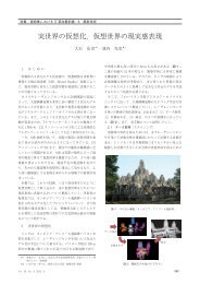
elements mass (kg) length (cm)head 4.90 25chest 18.06 40loins 12.04 20upper arm 2.52 25forearm 1.54 25hand 0.49 10thigh 7.98 40shank 3.71 40foot 1.26 25Table 3.1: The weight and length of rigid bodys• the force of 300N for 0.1 from the forward direction,• the force of a sinusoidal wave (100 sin(2πt) [N]) from the forwarddirection,• the force of 200N for 0.1 from the right direction.The analysis is performed every 0.01 second, and all perturbations act onnear the center of mass. The balance control is begun after 0.2 secondsince perturbations occur.3.3 ResultsThe results of the experiments are shown in Figure 3.1–3.4. In thefirst experiment, when the force of 500N acts from the back, the modelkeeps its balance by swinging its arms and bending down.The meaning of these is as the following. When the force acts, the28

angular momentum is generated and makes the model fall down forward.In order to reduce the effect of it, the model must generate the angularmomentum of the same direction, and the motion of swinging its armsand bending down is very effective for the purpose.These motions are often observed as the balance recovery motion byreal humans. They, probably empirically, select these motion for keepingtheir balance.In the second experiment, when the force of 300N acts form thefront, the model also swing its arms to keep its balance. In this case,the direction of the force is opposite from the previous case, and thenthe rotation of the arms is opposite, too. Because the waist cannot bendbackward as much as forward, the arms must be swung more than theprevious case.In the third experiment, the force of a sinusoidal wave always actson the model. The frequency of it is 1Hz. In this case, the PD control isusually chosen, and sometimes, when the model cannot keep its balanceby the PD control, the quadratic programming method is chosen and thearms are quickly moved for adjusting the angular momentum acting onthe model.In the last experiment, the force of 200N acts from the right sidedirection.The model also keeps its balance by swing its arms in thiscase. However, when the force acts from the side directions, the modelcan keep its balance against the smaller force than when it acts from thefront or the back. It is probably because there are a fewer DOF in the29

direction of the sides than in the direction of the front and the back.30

0.0sec 0.2sec 0.4sec 0.6sec0.8sec 1.0sec 1.2sec 1.4sec1.6sec1.8secFigure 3.1: The result (1)31

0.0sec 0.2sec 0.4sec 0.6sec0.8sec 1.0sec 1.2sec 1.4sec1.6sec 1.8sec 2.0sec 2.2sec2.4sec 2.6sec 2.8sec 3.0sec3.2sec 3.4sec 3.6sec 3.8secFigure 3.2: The result (2)32

0.0sec 0.2sec 0.4sec 0.6sec0.8sec 1.0sec 1.2sec 1.4sec1.6sec 1.8sec 2.0sec 2.2sec2.4sec 2.6sec 2.8sec 3.0sec3.2sec 3.4sec 3.6sec 3.8secFigure 3.3: The result (3)33

0.0sec 0.2sec 0.4sec 0.6sec0.8secFigure 3.4: The result (4)34

4 ConclusionsIn this thesis, a new algorithm for the postural adjustment of the humanbody model is proposed and implemented. This method is a feedbacksystem and can deal with large perturbations. It switches two methodsto generate motions; one uses the quadratic programming method andthe other uses the PD control. The former is for large perturbations andthe latter is for small perturbations or final posture adjustment.Thechoice of them depends on the position of the center of mass.In the experiments, the motion which is similar to the real humanmotion appeared, such as swinging the arms and bending down.Weempirically know that these motion are effective for keeping our balance,and this fact is experimentally confirmed by the proposed optimizationcalculation.35

5 Future workIn the proposed algorithm, the feet must touch the ground and cannotmove. However, this constraint is too strong. When a large perturbationis applied, stepping motion is usually selected for preventing the bodyfrom falling down. Therefore, it is desirable that the algorithm allows thestepping motion.Moreover, although only standing upright is permitted for the initialposture in this algorithm, it is not a reasonable constraints from theviewpoint of the applications of this algorithm. In the future, the algorithmwill be able to deal with various situations, such as the perturbationduring the gait.36

References[1] Horak F.B. and Nashner L.M. Central programming of posturalmovements: adaptation to altered support-surface configurations.Journal of Neurophysiology, 55:1369–1381, 1986.[2] Michael Gleicher. Retargetting motion to new characters. ComputerGraphicsi Proceedings, Annual Conference Series, pages 33–42, 1998.[3] Akimasa Ishida and Shinji Miyazaki. Maximum likelihood identificationof a posture control system. IEEE Transactions on BiomedicalEngineering, BME-34(1):1–5, 1987.[4] Hyeongseok Ko and Norman I. Badler. Animating human locomotionwith inverse dynamics. IEEE Computer Graphics and Applications,March:50–59, 1996.[5] Taku Komura, Yoshihisa Shinagawa, and Tosiyasu L. Kunii. Creatingand retargetting motion by the musculoskeletal human bodymodel. The Visual Computer, (5):254–270, 2000.[6] Arthur D. Kuo and Felix E. Zajac. Human standing posture:Multi-joint movement strategies based on biomechanical constraints.Progress in Brain Research, 97, 2000.[7] Joseph Laszlo, Michiel van de Panne, and Eugene Fiume. Limit cyclecontrol and its application to the animation of balancing and walk-37

ing. Computer Graphics (Proceedings of SIGGRAPH 96), 30:155–162, 1996.[8] Woollacott M.H., von Hosten C, and R ösblad B. Fixed patterns ofrapid postural responses among leg muscles during stance. ExperimentalBrain Research, 30:13–24, 1977.[9] Moore S.P., Rushmer D.S., Windus S.L., and Nashner L.M. Humanautomatic postural responses: responses to horizontal perturbationsof stance in multiple directions. Experimental Brain Research,73:648–658, 1988.[10] Seyoon Tak, Oh young Song, and Hyeong-Seok Ko. Motion balancefiltering. Computer Graphics Forum, 19(3), 2000.[11] Wayne Wooten. Simulations of Leaping, Tumbling, Landing, andBalancing Humans. PhD thesis, Georgia Institue of Technology,1997.[12] M. Oshita and A. makinouchi. A Dynamic Motion Control Techniquefor Human-like Articulated Figures. Eurotraphics 2001, vol.20,Number3, 2001[13] Mian-Ju Gu, Albert B. Schults, Nei T. Shepard and Neil B. Alexander.Postural control in young and elderly adults when stance is perturbed:Dynamics. Jounal of Biomechanics, 29(3), 319–329, 1996[14] S. Rietdyk, A.E. Patla, D.A. Winter, M.G.Ishac, C.E. Little. Balancerecoverty from medio-lateral perturbations of the upper body duringstanding. Journal of Biomechanics, 32:1149–1158, 1999[15] M.C.Do, C.Schneider, R.K.Y.Chong. Factors influencing the quickonset of stepping follwing postural perturbation. Journal of Biomechanics,32:795–802, 199938

[16] Elizabeth T. Hsiao, Stephen N. Robinovitch. Biomechanical influenceson balance recovery by stepping. Journal of Biomechanics,32:1099–1106, 1999[17] Yi-Chung Pai and James Patton. Center of mass velocity-positionpredictions for balance control. Journal of Biomechanics, 30(4), 347–354, 1997[18] Yi-Chung Pa, Kamran Iqbal. Simulated movement termination forbalance recovery: can movement strategies be sought to maintainstability in the persence of slipping or forced sliding? Journal ofBiomechanics, 32:779–786, 1999[19] Elisabetta Papa, Aurelio Cappozzo. A telescopic inverted-pendulummodel of the musculo-skeletarl system and its use for the analysis ofthe sit-to-stand motor task. Jounal of Biomechanics, 32:1205–1212,1999[20] K. Yamane and Y. Nakamura. Dynamics Filter — Concept and Implementationof On-Line Motion Generator for Human Figures. Proceedingsof the IEEE International Conference on Robotics and Automation,pp.688-695, 2000[21] S. Kagami, F. Kanehiro, Y. Yamiya, M. Inaba and H. Inoue. AutoBalancer: An Online Dynamic Balance Compensation Scheme forHumanoid Robots. Proceedings of The Fourth International Workshopon Algorithmic Foundations of Robotics (WAFR 2000), 200039