Mohamad-Ziad Charif - Antares
Mohamad-Ziad Charif - Antares Mohamad-Ziad Charif - Antares
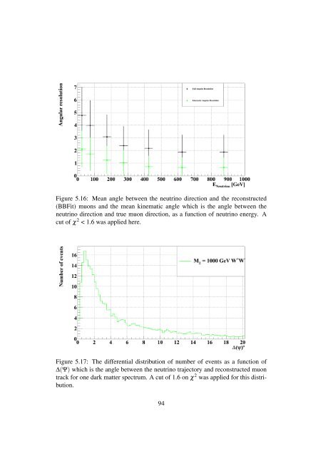
Figure 5.16: Mean angle between the neutrino direction and the reconstructed(BBFit) muons and the mean kinematic angle which is the angle between theneutrino direction and true muon direction, as a function of neutrino energy. Acut of χ 2 < 1.6 was applied here.Figure 5.17: The differential distribution of number of events as a function of∆(Ψ) which is the angle between the neutrino trajectory and reconstructed muontrack for one dark matter spectrum. A cut of 1.6 on χ 2 was applied for this distribution.94
n ν =E=M χˆE minn signal = n ν + n ¯ν[ ]dNνdE .Aν e f f ·t livetime.dE(5.3)n ¯ν =E=M χˆE min[ ]dN¯νdE .A e ¯ν f f ·t livetime.dE(5.4)The average upper limit as it is defined in equation 5.2 stands for the upperlimit µ ( n detected ,n expected)calculated with the Feldman-Cousins method andweighted by its Poisson probability, the n bgd variable stands for the expected numberof background, and j for the detected number of background.5.7.2 Search variables and optimizationsAs we previously saw, the half-cone angle between the direction of the Sun andthe direction of the reconstructed muon is a good discriminator between a darkmatter neutrino signal and the background, this can be seen again in figure 5.18.In addition if we look at figure 5.19 where we have the track χ 2 distribution ofour background and our signal, we can see that for up-going events such as atmosphericneutrinos and the dark matter neutrino signal they have the same shape butthe down-going muons that are reconstructed as up-going have a distinct shape.Thus the χ 2 variable will help us separate the badly reconstructed down-goingmuons (which dominates our data) and our up-going events which contains atmosphericneutrinos and a possible dark matter neutrino signal. The effect of othervariables such as N hit , or bchi2 are assumed to be minimal and will not be used inthis optimization.As consequence, these two variables (half-cone angle ∆(Ψ), χ 2 ) will be usedto minimize the sensitivity to a dark matter signal. The search for the optimalpoint in (∆(Ψ), χ 2 ) will be done by fixing the χ 2 at a certain value and searchfor the ∆(Ψ) cut that gives the lowest sensitivity, and then repeat the calculationfor a different value of χ 2 . This iterative process is then done for all availableWIMP spectra in order to find the best sensitivity for each dark matter model. Thesearch region for the χ 2 variable would be between χ 2 = 1.2 and χ 2 = 2 , and asfor ∆(Ψ) it would be between ∆(Ψ) = 0 ◦ and ∆(Ψ) = 10 ◦ .Looking back at figure 5.19 we can expect to find the same χ 2 cut for all darkmatter spectrum regardless of its mass or what annihilation channels, as they allshare the same shape. This is indeed what is found as a result of the optimizationas we can see in figure 5.21 where we can see the result of the difference of theoptimized values for the sensitivity for two example spectrum . Now if we take95
- Page 46 and 47: 3.2.1.1 Detector layoutOptical Modu
- Page 48 and 49: • The LED (light emitting diode)
- Page 50 and 51: Anchor & BuoyEach line is anchored
- Page 52 and 53: Figure 3.17: Distribution of azimut
- Page 54 and 55: Figure 3.20: Height and radial disp
- Page 56 and 57: Figure 3.22: Distribution of sea cu
- Page 58 and 59: Figure 3.24: Time offset among OMs
- Page 60 and 61: Figure 3.26: Distribution of time d
- Page 62 and 63: Line number Connection Date Mainten
- Page 64 and 65: Figure 3.29: Comparison between sky
- Page 66 and 67: Figure 3.31: The effective area for
- Page 68 and 69: Figure 4.1: Median counting rate of
- Page 70 and 71: Figure 4.4: Average neutrino events
- Page 72 and 73: 2. All hits on the same floor are m
- Page 74 and 75: 4.2.1 Neutrino simulationFigure 4.6
- Page 76 and 77: • Multiplicity range of the muon
- Page 78 and 79: Chapter 5Dark Matter search in the
- Page 80 and 81: Figure 5.2: Annihilation spectrum f
- Page 82 and 83: Livetime(days) 5 Lines 9 Lines 10 L
- Page 84 and 85: Figure 5.4: Monte Carlo Truth distr
- Page 86 and 87: Figure 5.7: Tchi2 distribution for
- Page 88 and 89: Figure 5.9: Tchi2 distribution for
- Page 90 and 91: Figure 5.11: Sun’s position taken
- Page 92 and 93: Figure 5.13: Comparison between the
- Page 94 and 95: Figure 5.15: Estimation of the back
- Page 98 and 99: Figure 5.18: A comparison of the di
- Page 100 and 101: a look at figure 5.22 we find a cle
- Page 102 and 103: The resulting optimized sensitiviti
- Page 104 and 105: Figure 5.26: A comparison plot of t
- Page 106 and 107: dΦ µdE ν= dΦ νdE νP earth ρN
- Page 108 and 109: Figure 5.31: Limits on the muon flu
- Page 110 and 111: Chapter 6Dark Matter search in the
- Page 112 and 113: Figure 6.1: . True Position of the
- Page 114 and 115: Figure 6.3: Comparison of the three
- Page 116 and 117: For BBFit all variables mentioned i
- Page 118 and 119: Figure 6.6: The distribution of χ
- Page 120 and 121: annihilation channel W + W − the
- Page 122 and 123: lowering the total contribution of
- Page 124 and 125: 6.4.2 BBFit Single-line analysisThe
- Page 126 and 127: Figure 6.15: Comparison between the
- Page 128 and 129: Figure 6.17: Comparison of Nhit dis
- Page 130 and 131: Figure 6.19: The estimation of the
- Page 132 and 133: Figure 6.21: Comparison of the opti
- Page 134 and 135: Figure 6.23: Comparison of sensitiv
- Page 136 and 137: Figure 6.25: Estimation of our back
- Page 138 and 139: Figure 6.28: Comparison of the mult
- Page 140 and 141: Figure 6.29: Comparison of the Λ d
- Page 142 and 143: Figure 6.31: Comparison of the cos(
- Page 144 and 145: Figure 6.34: Comparison of the esti
Figure 5.16: Mean angle between the neutrino direction and the reconstructed(BBFit) muons and the mean kinematic angle which is the angle between theneutrino direction and true muon direction, as a function of neutrino energy. Acut of χ 2 < 1.6 was applied here.Figure 5.17: The differential distribution of number of events as a function of∆(Ψ) which is the angle between the neutrino trajectory and reconstructed muontrack for one dark matter spectrum. A cut of 1.6 on χ 2 was applied for this distribution.94


