Mohamad-Ziad Charif - Antares
Mohamad-Ziad Charif - Antares Mohamad-Ziad Charif - Antares
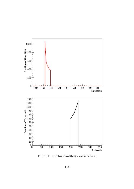
Figure 6.1: . True Position of the Sun during one run.110
Figure 6.2: . Comparison of two different methods to calculate the position of theSun in local coordinates (Elevation). First method is with both δ and RA fixed(red curve) while the other is with δ fixed and RA randomized (black curve).1. For each run calculate the value of δ of the Sun at mid-run time, and use itwith GENHEN point source mode to create the ν/ ¯ν MC.2. Calculate the region where the Sun occupies in local coordinates (Zenith ,Azimuth) during the run and remove events from the MC that are outsidethis region.3. For different M χ we remove events that have E ν > M χ .4. We apply for each dark matter model the corresponding dNdEto the remainingevents by re-weighting the MC event spectrum via a convolution with theeffective area of the detector.After applying this method we get the following distribution of our MC signal infigures 6.4 & 6.5 .6.2 Reconstruction StrategyFor this analysis both AAFit and BBFit reconstruction strategies will be used.And later in section 6.6 we will present a comparison of the two strategies and theimplications on presented sensitivities and limits.111
- Page 62 and 63: Line number Connection Date Mainten
- Page 64 and 65: Figure 3.29: Comparison between sky
- Page 66 and 67: Figure 3.31: The effective area for
- Page 68 and 69: Figure 4.1: Median counting rate of
- Page 70 and 71: Figure 4.4: Average neutrino events
- Page 72 and 73: 2. All hits on the same floor are m
- Page 74 and 75: 4.2.1 Neutrino simulationFigure 4.6
- Page 76 and 77: • Multiplicity range of the muon
- Page 78 and 79: Chapter 5Dark Matter search in the
- Page 80 and 81: Figure 5.2: Annihilation spectrum f
- Page 82 and 83: Livetime(days) 5 Lines 9 Lines 10 L
- Page 84 and 85: Figure 5.4: Monte Carlo Truth distr
- Page 86 and 87: Figure 5.7: Tchi2 distribution for
- Page 88 and 89: Figure 5.9: Tchi2 distribution for
- Page 90 and 91: Figure 5.11: Sun’s position taken
- Page 92 and 93: Figure 5.13: Comparison between the
- Page 94 and 95: Figure 5.15: Estimation of the back
- Page 96 and 97: Figure 5.16: Mean angle between the
- Page 98 and 99: Figure 5.18: A comparison of the di
- Page 100 and 101: a look at figure 5.22 we find a cle
- Page 102 and 103: The resulting optimized sensitiviti
- Page 104 and 105: Figure 5.26: A comparison plot of t
- Page 106 and 107: dΦ µdE ν= dΦ νdE νP earth ρN
- Page 108 and 109: Figure 5.31: Limits on the muon flu
- Page 110 and 111: Chapter 6Dark Matter search in the
- Page 114 and 115: Figure 6.3: Comparison of the three
- Page 116 and 117: For BBFit all variables mentioned i
- Page 118 and 119: Figure 6.6: The distribution of χ
- Page 120 and 121: annihilation channel W + W − the
- Page 122 and 123: lowering the total contribution of
- Page 124 and 125: 6.4.2 BBFit Single-line analysisThe
- Page 126 and 127: Figure 6.15: Comparison between the
- Page 128 and 129: Figure 6.17: Comparison of Nhit dis
- Page 130 and 131: Figure 6.19: The estimation of the
- Page 132 and 133: Figure 6.21: Comparison of the opti
- Page 134 and 135: Figure 6.23: Comparison of sensitiv
- Page 136 and 137: Figure 6.25: Estimation of our back
- Page 138 and 139: Figure 6.28: Comparison of the mult
- Page 140 and 141: Figure 6.29: Comparison of the Λ d
- Page 142 and 143: Figure 6.31: Comparison of the cos(
- Page 144 and 145: Figure 6.34: Comparison of the esti
- Page 146 and 147: The optimal Λ cut for all dark mat
- Page 148 and 149: Figure 6.40: Sensitivity to neutrin
- Page 150 and 151: 6.7 Comparison with 2007-2008 analy
- Page 152 and 153: mass of 200 GeV and a cross-section
- Page 154 and 155: Chapter 7ConclusionsThe limits pres
- Page 156 and 157: Bibliography[1] Volders, L. M. J. S
- Page 158 and 159: [22] S. Burles et al., “Big bang
- Page 160 and 161: [46] G. Debrassi, S. Heinemeyer, W.
Figure 6.1: . True Position of the Sun during one run.110


