FOR DIFFERENTIAL EQUATIONS OF FRACTIONAL ORDER

More documents

Recommendations

Info

76 T. S. Aleroev, H. T. Aleroeva, Ning-Ming Nie, and Yi-Fa TangAccording to the above lemma, we get the error estimate∣∣y(t; ξ ∗ ) − y(t; ˜ξ) ∣ ∣ ≤≤ |ξ ∗ − ˜ξ|(t − a)E α (K f (t − a) α ) ≤ C 1 |ξ ∗ − ˜ξ|, t ∈ [a, b], (3.61)where C 1 := max (t − a)E α(K f (t − a) α ).t∈[a,b]Another part of the error is from numerical solving procedure of FIVP(3.50) by scheme (3.33), (3.35). Suppose that the scheme of FIVP convergeswith order r, and denote the approximate solution of y(t n ; ˜ξ) as y n (˜ξ). Weget ∃ C 2 > 0, s.t.∣max ∣y(t n ; ˜ξ) − y n (˜ξ) ∣ ≤ C 2 h r . (3.62)0≤n≤NTo sum up, we have∣∣y(t n ; ξ ∗ ) − y n (˜ξ) ∣ ∣ = ∣ ∣y(t n ; ξ ∗ ) − y(t n ; ˜ξ) + y(t n ; ˜ξ) − y n (˜ξ) ∣ ∣ ≤that is,≤ ∣ ∣y(t n ; ξ ∗ ) − y(t n ; ˜ξ) ∣ ∣ + ∣ ∣y(t n ; ˜ξ) − y n (˜ξ) ∣ ∣max0≤n≤N∣∣y(t n ; ξ ∗ ) − y n (˜ξ) ∣ ≤ C 1 |ξ ∗ − ˜ξ| + C 2 h r . (3.63)As to (3.7), (3.41), we turn it into its corresponding FIVPRLa D γ t y(t) + f (t, y(t)) = 0, a ≤ t ≤ b, 1 < γ ≤ 2, (3.64)RLa D γ−1t y(t) ∣ = ξ, lim J 2−γt=a t→a + a y(t) = 0. (3.65)The numerical procedure of simulating (3.7), (3.41) is completely similar tothat of (3.1), (3.41).Again, the procedures of shooting method for (3.2) and (3.8) with homogenousboundary conditions (3.41) are similar to the case of (3.1), (3.41)and (3.7), (3.41), respectively.4. Numerical Experiments for Solving FBVPsIn this section, two numerical examples are given to show the feasibilityand validity of single shooting methods for the FBVPs.First, let us introduce the parameters. a = 0 = t 0 < t 1 < · · · < t n = bis a given equispaced mesh with stepsize h = (b − a)/n, n = 100, γ = 1.5,θ = 0.5. For the linear cases in Examples 1, the two “initial speeds” ξ 1 = 0.5,ξ 2 = 1.5. For the nonlinear cases in Examples 2, ɛ = 10 −12 , ξ (0) = 0,△ξ (k) ≡ 10 −8 .Example 3.1. Consider the following linear FBVPC0 D 1.5C0 D 0.5t y(t) + 1 3 y(t) + 1 4t y(t) = r(t), 0 < t < 1,y(0) = 0, y(1) = 0,
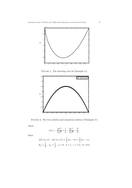
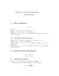
Boundary Value Problems for Differential Equations of Fractional Order 770 x 10−4−0.5−1error−1.5−2−2.5−30 0.1 0.2 0.3 0.4 0.5 0.6 0.7 0.8 0.9 1tFigure 1. The shooting error for Example 3.10.35numerical solutionanalytical solution0.30.250.2y(t)0.150.10.0500 0.1 0.2 0.3 0.4 0.5 0.6 0.7 0.8 0.9 1tFigure 2. The true solution and numerical solution of Example 3.1whereSincer(t) = − 7t0.52 √ π + t 3 − 2t1.53 √ π − t2 3 .∣∣g(t, u 2 , v 2 ) − g(t, u 1 , v 1 ) ∣ ∣ ≤ 1 3 |u 2 − u 1 | + 1 4 |v 2 − v 1 |,K g = 1 3 , L g = 1 , a = 0, b = 1, γ = 1.5, θ = 0.5,4
Page 4 and 5:
24 T. S. Aleroev, H. T. Aleroeva, N
Page 8 and 9: 28 T. S. Aleroev, H. T. Aleroeva, N
Page 20 and 21: CHAPTER 2The Sturm-Liouville Proble
Page 46 and 47: CHAPTER 3Solving Two-Point Boundary
Page 58 and 59: Since∣∣f(t, u 2 ) − f(t, u 1
Page 60 and 61: agreement with the fact that (3.33)
Page 62: 82 T. S. Aleroev, H. T. Aleroeva, N
show all

FOR DIFFERENTIAL EQUATIONS OF FRACTIONAL ORDER

You also want an ePaper? Increase the reach of your titles

Delete template?

Save as template?