FEniCS Course - FEniCS Project

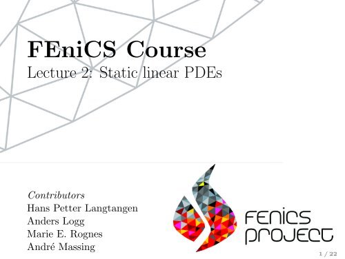
FEniCS CourseLecture 2: Static linear PDEsContributorsHans Petter LangtangenAnders LoggMarie E. RognesAndré Massing1 / 22

Hello World!We will solve Poisson’s equation, the Hello World of scientificcomputing:−∆u = fu = u 0in Ωon ∂ΩPoisson’s equation arises in numerous contexts:• heat conduction, electrostatics, diffusion of substances,twisting of elastic rods, inviscid fluid flow, water waves,magnetostatics• as part of numerical splitting strategies of morecomplicated systems of PDEs, in particular theNavier–Stokes equations2 / 22

The FEM cookbookAu = f(i)Partial differential equationMultiply by vTake V h ⊂ VLet u h = ∑ j U jφ j(ii)a(u, v) = L(v) Continuous variational problem(iii)a(u h , v) = L(v) Discrete variational problem(iv)AU = b System of discrete equations3 / 22

Solving PDEs in FEniCSSolving a physical problem with FEniCS consists of thefollowing steps:1 Identify the PDE and its boundary conditions2 Reformulate the PDE problem as a variational problem3 Make a Python program where the formulas in thevariational problem are coded, along with definitions ofinput data such as f, u 0 , and a mesh for Ω4 Add statements in the program for solving the variationalproblem, computing derived quantities such as ∇u, andvisualizing the results4 / 22

Deriving a variational problem for Poisson’sequationThe simple recipe is: multiply the PDE by a test function v andintegrate over Ω:∫∫− (∆u)v dx = fv dxΩΩThen integrate by parts and set v = 0 on the Dirichletboundary:∫∫∫∂u− (∆u)v dx = ∇u · ∇v dx −ΩΩ∂Ω ∂n v ds} {{ }=0We find that:∫Ω∫∇u · ∇v dx =Ωfv dx5 / 22

Variational problem for Poisson’s equationFind u ∈ V such that∫for all v ∈ ˆVΩ∫∇u · ∇v dx =Ωfv dxThe trial space V and the test space ˆV are (here) given byV = {v ∈ H 1 (Ω) : v = u 0 on ∂Ω}ˆV = {v ∈ H 1 (Ω) : v = 0 on ∂Ω}6 / 22

Discrete variational problem for Poisson’sequationWe approximate the continuous variational problem with adiscrete variational problem posed on finite dimensionalsubspaces of V and ˆV :V h ⊂ VˆV h ⊂ ˆVFind u h ∈ V h ⊂ V such that∫∫∇u h · ∇v dx =for all v ∈ ˆV h ⊂ ˆVΩΩfv dx7 / 22

Canonical variational problemThe following canonical notation is used in FEniCS: find u ∈ Vsuch thata(u, v) = L(v)for all v ∈ ˆVFor Poisson’s equation, we have∫a(u, v) = ∇u · ∇v dx∫ΩL(v) = fv dxΩa(u, v) is a bilinear form and L(v) is a linear form8 / 22

A test problemWe construct a test problem for which we can easily check theanswer. We first define the exact solution byu(x, y) = 1 + x 2 + 2y 2We insert this into Poisson’s equation:f = −∆u = −∆(1 + x 2 + 2y 2 ) = −(2 + 4) = −6This technique is called the method of manufactured solutions9 / 22

Implementation in FEniCSfrom dolfin import *mesh = UnitSquareMesh (8, 8)V = FunctionSpace (mesh , " Lagrange ", 1)u0 = Expression ("1 + x[0]*x[0] + 2*x[1]*x[1]")bc = DirichletBC (V, u0 , " on_boundary ")f = Constant (-6.0)u = TrialFunction (V)v = TestFunction (V)a = inner ( grad (u), grad (v))*dxL = f*v*dxu = Function (V)solve (a == L, u,bc)plot (u)interactive ()10 / 22

Step by step: the first lineThe first line of a FEniCS program usually begins withfrom dolfin import *This imports key classes like UnitSquare, FunctionSpace,Function and so forth, from the FEniCS user interface(DOLFIN)11 / 22

Step by step: creating a meshNext, we create a mesh of our domain Ω:mesh = UnitSquare (8, 8)Defines a mesh of 8 × 8 × 2 = 128 triangles of the unit squareOther useful classes for creating meshes includeUnitIntervalMesh, UnitCubeMesh, UnitCircleMesh,UnitSphereMesh, RectangleMesh and BoxMeshComplex geometries can be built using Constructive Solid Geometry(CSG) which is built into FEniCS (operators +, -, *):r = Rectangle (0.5, 0.5, 1.5, 1.5)c = Circle (1, 1, 1)...g = (r - c)*b + amesh = Mesh (g)12 / 22

Step by step: creating a function spaceThe following line creates a function space on Ω:V = FunctionSpace (mesh , " Lagrange ", 1)The second argument specifies the type of element, while thethird argument is the degree of the basis functions on theelementOther types of elements include "Discontinuous Lagrange","Brezzi-Douglas-Marini", "Raviart-Thomas","Crouzeix-Raviart", "Nedelec 1st kind H(curl)" and"Nedelec 2nd kind H(curl)"13 / 22

Step by step: defining expressionsNext, we define an expression for the boundary value:u0 = Expression ("1 + x[0]*x[0] + 2*x[1]*x[1]")The formula must be written in C++ syntaxOptionally, a polynomial degree may be specifiedu0 = Expression ("1 + x[0]*x[0] + 2*x[1]*x[1]",degree =2)The Expression class is very flexible and can be used to createcomplex user-defined expressions. For more information, tryhelp ( Expression )in Python or, in the shell:pydocdolfin . Expression14 / 22

Step by step: defining a boundary conditionThe following code defines a Dirichlet boundary condition:bc = DirichletBC (V, u0 , " on_boundary ")This boundary condition states that a function in the functionspace defined by V should be equal to u0 on the domain definedby "on boundary"Note that the above line does not yet apply the boundarycondition to all functions in the function space15 / 22

Step by step: more about defining domainsFor a Dirichlet boundary condition, a simple domain can be definedby a string" on_boundary " # The entire boundaryAlternatively, domains can be defined by subclassing SubDomainclass Boundary ( SubDomain ):def inside (self , x, on_boundary ):return on_boundaryYou may want to experiment with the definition of the boundary:" near (x[0], 0.0)" # x_0 = 0" near (x[0], 0.0) || near (x[1], 1.0)"There are many more possibilities, seehelp ( SubDomain )help ( DirichletBC )16 / 22

Step by step: defining the right-hand sideThe right-hand side f = −6 may be defined as follows:f = Expression ("-6")or (more efficiently) asf = Constant (-6.0)17 / 22

Step by step: defining variational problemsVariational problems are defined in terms of trial and testfunctions:u =v =TrialFunction (V)TestFunction (V)We now have all the objects we need in order to specify thebilinear form a(u, v) and the linear form L(v):a = inner ( grad (u), grad (v))*dxL = f*v*dx18 / 22

Step by step: solving variational problemsOnce a variational problem has been defined, it may be solvedby calling the solve function:u = Function (V)solve (a == L, u,bc)Note the reuse of the variable u as both a TrialFunction inthe variational problem and a Function to store the solution19 / 22

Step by step: post-processingThe solution and the mesh may be plotted by simply calling:plot (u)plot ( mesh )interactive ()The interactive() call is necessary for the plot to remain onthe screen and allows the plots to be rotated, translated andzoomedFor postprocessing in ParaView or MayaVi, store the solutionin VTK format:file = File (" poisson . pvd ")file

Python/FEniCS programming 1011 Open a file with your favorite text editor (Emacs :-) andname the file something like test.py2 Write the following in the file and save it:from dolfin import *print dolfin . __version__3 Run the file/program by typing the following in a terminal(with FEniCS setup):pythontest .py21 / 22

The FEniCS challenge!Solve the partial differential equation−∆u = fwith homogeneous Dirichlet boundary conditions on the unitsquare for f(x, y) = 2π 2 sin(πx) sin(πy). Plot the error in the L 2norm as function of the mesh size h for a sequence of refinedmeshes. Try to determine the convergence rate.• Who can obtain the smallest error?• Who can compute a solution with an error smaller thanɛ = 10 −6 in the fastest time?The best students(s) will be rewarded with an exclusive FEniCSsurprise!Hint: help(errornorm)22 / 22