Metrics of curves in shape optimization and analysis - Andrea Carlo ...

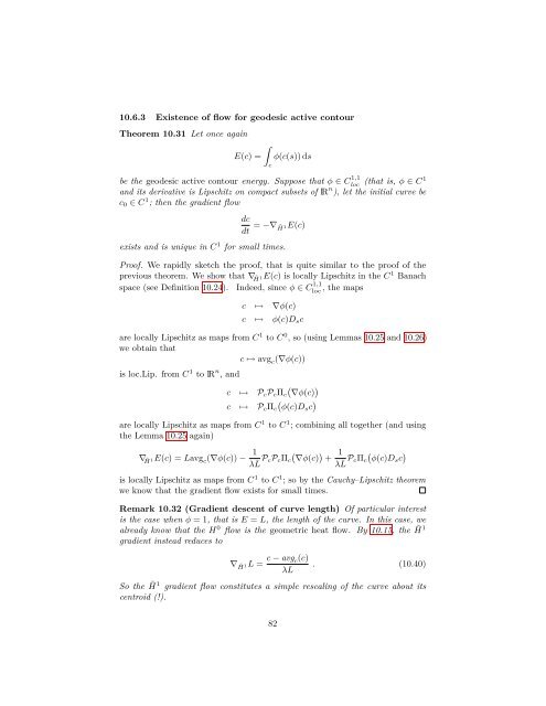
10.6.3 Existence of flow for geodesic active contourTheorem 10.31 Let once again∫E(c) = φ(c(s)) dscbe the geodesic active contour energy. Suppose that φ ∈ C 1,1loc(that is, φ ∈ C1and its derivative is Lipschitz on compact subsets of lR n ), let the initial curve bec 0 ∈ C 1 ; then the gradient flowdc= −∇dt˜H1E(c)exists and is unique in C 1 for small times.Proof. We rapidly sketch the proof, that is quite similar to the proof of theprevious theorem. We show that ∇˜H1E(c) is locally Lipschitz in the C 1 Banachspace (see Definition 10.24). Indeed, since φ ∈ C 1,1loc, the mapsc ↦→ ∇φ(c)c ↦→ φ(c)D s care locally Lipschitz as maps from C 1 to C 0 , so (using Lemmas 10.25 and 10.26)we obtain thatc ↦→ avg c (∇φ(c))is loc.Lip. from C 1 to lR n , andc ↦→ P c P c Π c(∇φ(c))c ↦→ P c Π c(φ(c)Ds c )are locally Lipschitz as maps from C 1 to C 1 ; combining all together (and usingthe Lemma 10.25 again)∇˜H1E(c) = Lavg c (∇φ(c)) − 1λL P cP c Π c(∇φ(c))+1λL P cΠ c(φ(c)Ds c )is locally Lipschitz as maps from C 1 to C 1 ; so by the Cauchy–Lipschitz theoremwe know that the gradient flow exists for small times.Remark 10.32 (Gradient descent of curve length) Of particular interestis the case when φ = 1, that is E = L, the length of the curve. In this case, wealready know that the H 0 flow is the geometric heat flow. By 10.15, the ˜H 1gradient instead reduces to∇ ˜H1L = c − avg c(c)λL. (10.40)So the ˜H 1 gradient flow constitutes a simple rescaling of the curve about itscentroid (!).82