Metrics of curves in shape optimization and analysis - Andrea Carlo ...

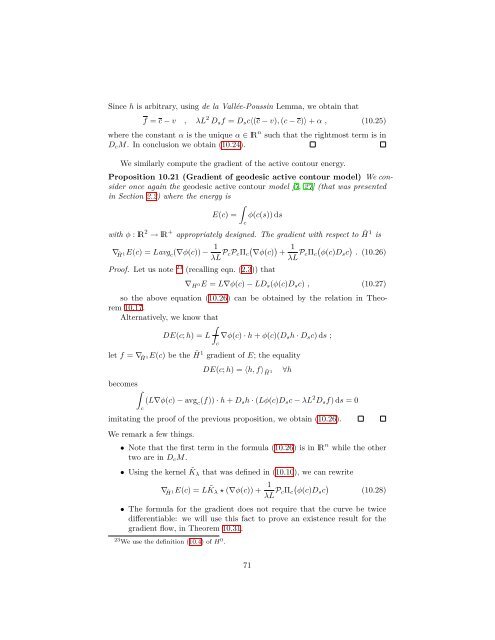
Since h is arbitrary, using de la Vallée-Poussin Lemma, we obtain thatf = c − v , λL 2 D s f = D s c〈(c − v), (c − c)〉 + α , (10.25)where the constant α is the unique α ∈ lR n such that the rightmost term is inD c M. In conclusion we obtain (10.24).We similarly compute the gradient of the active contour energy.Proposition 10.21 (Gradient of geodesic active contour model) We consideronce again the geodesic active contour model [7, 27] (that was presentedin Section 2.2) where the energy is∫E(c) = φ(c(s)) dscwith φ : lR 2 → lR + appropriately designed. The gradient with respect to ˜H 1 is∇˜H1E(c) = Lavg c (∇φ(c)) − 1λL P cP c Π c(∇φ(c))+1λL P cΠ c(φ(c)Ds c ) . (10.26)Proof. Let us note 23 (recalling eqn. (2.3)) that∇ H 0E = L∇φ(c) − LD s (φ(c)D s c) , (10.27)so the above equation (10.26) can be obtained by the relation in Theorem10.17.Alternatively, we know that∫DE(c; h) = L ∇φ(c) · h + φ(c)(D s h · D s c) ds ;let f = ∇˜H1E(c) be the ˜H 1 gradient of E; the equalitycDE(c; h) = 〈h, f〉 ˜H1∀hbecomes ∫(L∇φ(c) − avg c (f)) · h + D s h · (Lφ(c)D s c − λL 2 D s f) ds = 0cimitating the proof of the previous proposition, we obtain (10.26).We remark a few things.• Note that the first term in the formula (10.26) is in lR n while the othertwo are in D c M.• Using the kernel ˜Kλ that was defined in (10.10), we can rewrite∇˜H1E(c) = L ˜K λ ⋆ (∇φ(c)) + 1λL P cΠ c(φ(c)Ds c ) (10.28)• The formula for the gradient does not require that the curve be twicedifferentiable: we will use this fact to prove an existence result for thegradient flow, in Theorem 10.31.23 We use the definition (10.4) of H 0 .71