Metrics of curves in shape optimization and analysis - Andrea Carlo ...
Metrics of curves in shape optimization and analysis - Andrea Carlo ... Metrics of curves in shape optimization and analysis - Andrea Carlo ...
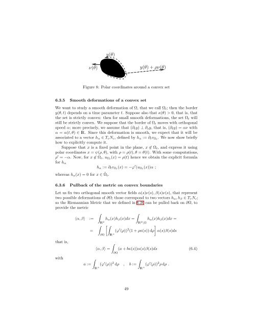
of a small ball from A. The motion v At inside N c is Lipschitz, but the limitlimt→0+v At − v A‖v At − v A ‖ L pdoes not exist in L p . (Morally, if p = 1, the limit would be the measure δ x ).6.3.3 Riemannian metricLet now p = 2. The set N c may fail to be a smooth submanifold of L 2 ; yetwe will, as much as possible, pretend that it is, in order to induce a sort of“Riemannian metric” on N c from the standard L 2 metric.Definition 6.20 We define the “Riemannian metric” on N c simply by〈h, k〉 := 〈h, k〉 L 2for h, k ∈ T v N c and correspondingly a norm bywhere T v N c is the contingent cone.|h| := √ 〈h, h〉Proposition 6.21 The distance induced by this “Riemannian metric” coincideswith the geodesically induce distance d g .The proof is in 3.22 in Duci and Mennucci [15].To conclude, we propose an explicit computation of the Riemannian Metricfor the case of compact sets in the plane with smooth boundaries; we then pullback the metric to obtain a metric of closed embedded planar curves. We startwith the case of convex sets.We fix p = 2, N = 2.6.3.4 Polar coordinates of smooth convex setsLet Ω ⊂ lR 2 be a convex set with smooth boundary; let y(θ) : [0, L] → ∂Ω bea parameterization of the boundary (by arc parameter), ν(θ) the unit vectornormal to ∂Ω and pointing external to Ω. The following “polar” change ofcoordinates ψ holds:ψ : lR + × [0, L] → lR \ Ω , ψ(ρ, θ) = y(θ) + ρν(θ) (6.3)see figure 8 on the following page. We suppose that y(θ) moves on ∂Ω inanticlockwise direction; so ν = J∂ s y, ∂ ss y = −κν; where J is the rotation matrix(of angle −π/2), κ is the curvature, and ∂ s y is the tangent vector.We can then express a generic integral through this change of coordinates as∫∫f(x) dx = f(ψ(ρ, s))|1 + ρκ(s)| dρ dslR 2 \Ω∫lR + ∂Ωwhere s is arc parameter, and ds is integration in arc parameter.48
y(θ)ν(θ)y(θ) + ρν(θ)Figure 8: Polar coordinates around a convex set6.3.5 Smooth deformations of a convex setWe want to study a smooth deformation of Ω, that we call Ω t ; then the bordery(θ, t) depends on a time parameter t. Suppose also that κ(θ) > 0, that is, thatthe set is strictly convex: then for small smooth deformations, the set Ω t willstill be strictly convex. We suppose that the border of Ω t moves with orthogonalspeed α; more precisely, we assume that (∂ t y) ⊥ ∂ s y, that is, (∂ t y) = αν withα = α(t, θ) ∈ lR. Since this deformation is smooth, we expect that it will beassociated to a vector h α ∈ T v N c , defined by h α := ∂ t v Ωt . We now show brieflyhow to explicitly compute it.Suppose that x is a fixed point in the plane, x ∉ Ω t , and express it usingpolar coordinates x = ψ(ρ, θ), with ρ = ρ(t), θ = θ(t). With some computations,ρ ′ = −α. Now, for x ∉ Ω t , u Ωt (x) = ρ(t) hence we obtain the explicit formulafor h αh α := ∂ t v Ωt (x) = −ϕ ′ (u Ωt (x))α ;whereas h α (x) = 0 for x ∈ ˚Ω t .6.3.6 Pullback of the metric on convex boundariesLet us fix two orthogonal smooth vector fields α(s)ν(s), β(s)ν(s), that representtwo possible deformations of ∂Ω; those correspond to two vectors h α , h β ∈ T v N c ;so the Riemannian Metric that we defined in 6.20 can be pulled back on ∂Ω, toprovide the metric∫∫〈α, β〉 := h α (x)h β (x)dx = h α (x)h β (x)dx =lR 2 lR 2 \Ω∫ [∫]=(ϕ ′ (ρ)) 2 (1 + ρκ(s)) dρ α(s)β(s)ds∂Ω lR +that is,with∫〈α, β〉 =∂Ω(a + bκ(s))α(s)β(s)ds (6.4)∫∫a := (ϕ ′ (ρ)) 2 dρlR + , b := (ϕ ′ (ρ)) 2 ρ dρ .lR +49
- Page 1 and 2: Metrics of curves in shape optimiza
- Page 3 and 4: shape analysis where we study a fam
- Page 5 and 6: • F (c) = F (c ◦ φ) for all cu
- Page 7 and 8: κ > 0HNNHNHκ < 0Figure 1: Example
- Page 9 and 10: In the case of planar curves c 1 ,
- Page 11 and 12: (a) (b) (c) (d) (e)Figure 3: Segmen
- Page 13 and 14: where φ may be chosen to beφ(x) =
- Page 15 and 16: 2.4.1 Example: geometric heat flowW
- Page 17 and 18: 2.4.5 Centroid energyWe will now pr
- Page 20 and 21: shapes. Unfortunately, H 0 does not
- Page 22 and 23: • If the second request is waived
- Page 24 and 25: • The Fréchet space of smooth fu
- Page 26 and 27: Since φ k are homeomorphisms, then
- Page 28 and 29: 3.6.1 Riemann metric, lengthDefinit
- Page 30 and 31: Theorem 3.30 Suppose that M is a sm
- Page 32 and 33: Example 3.38 Let M = C ∞ ([−1,
- Page 34 and 35: • sometimes S 1 will be identifie
- Page 36 and 37: The proof is by direct computation.
- Page 38 and 39: The term preshape space is sometime
- Page 40 and 41: 5 Representation/embedding/quotient
- Page 42 and 43: 6.1.1 Length induced by a distanceI
- Page 44 and 45: 0101200000000000011111111111110000
- Page 46 and 47: 6.2.4 Applications in computer visi
- Page 50 and 51: CutΩ(The arrows represent the dist
- Page 52 and 53: 7.3 L 1 metric and Plateau problemI
- Page 54 and 55: Definition 8.3 (Flat curves) Let Z
- Page 56 and 57: Proof. Fix α 0 ∈ S \ Z. Let T =
- Page 58 and 59: 8.2.2 RepresentationThe Stiefel man
- Page 60 and 61: 9.3 Conformal metricsYezzi and Menn
- Page 62 and 63: 10.1.1 Related worksA family of met
- Page 64 and 65: Definition 10.7 (Convolution) A arc
- Page 66 and 67: and̂∇˜HjE(0) = ̂∇ H 0E(0),̂
- Page 68 and 69: and we simply integrate twice! More
- Page 70 and 71: Corollary 10.18 In particular, the
- Page 72 and 73: 10.6 Existence of gradient flowsWe
- Page 74 and 75: • The length functional (from C 1
- Page 76 and 77: We can eventually estimate the diff
- Page 78 and 79: 7.552.5-10 -7.5 -5 -2.5 2.5 5 7.5 1
- Page 80 and 81: By using (i) and (ii) from lemma 10
- Page 82 and 83: 10.6.3 Existence of flow for geodes
- Page 84 and 85: 10.7.1 Robustness w.r.to local mini
- Page 86 and 87: We already presented all the calcul
- Page 88 and 89: 10.9 New regularization methodsTypi
- Page 90 and 91: can be solved for k (this is not so
- Page 92 and 93: 2. Now• at t = 1/2 it achieves th
- Page 94 and 95: Definition 11.10 • The orbit is O
- Page 96 and 97: y eqn. (11.3), where the terms RHS
y(θ)ν(θ)y(θ) + ρν(θ)Figure 8: Polar coord<strong>in</strong>ates around a convex set6.3.5 Smooth deformations <strong>of</strong> a convex setWe want to study a smooth deformation <strong>of</strong> Ω, that we call Ω t ; then the bordery(θ, t) depends on a time parameter t. Suppose also that κ(θ) > 0, that is, thatthe set is strictly convex: then for small smooth deformations, the set Ω t willstill be strictly convex. We suppose that the border <strong>of</strong> Ω t moves with orthogonalspeed α; more precisely, we assume that (∂ t y) ⊥ ∂ s y, that is, (∂ t y) = αν withα = α(t, θ) ∈ lR. S<strong>in</strong>ce this deformation is smooth, we expect that it will beassociated to a vector h α ∈ T v N c , def<strong>in</strong>ed by h α := ∂ t v Ωt . We now show brieflyhow to explicitly compute it.Suppose that x is a fixed po<strong>in</strong>t <strong>in</strong> the plane, x ∉ Ω t , <strong>and</strong> express it us<strong>in</strong>gpolar coord<strong>in</strong>ates x = ψ(ρ, θ), with ρ = ρ(t), θ = θ(t). With some computations,ρ ′ = −α. Now, for x ∉ Ω t , u Ωt (x) = ρ(t) hence we obta<strong>in</strong> the explicit formulafor h αh α := ∂ t v Ωt (x) = −ϕ ′ (u Ωt (x))α ;whereas h α (x) = 0 for x ∈ ˚Ω t .6.3.6 Pullback <strong>of</strong> the metric on convex boundariesLet us fix two orthogonal smooth vector fields α(s)ν(s), β(s)ν(s), that representtwo possible deformations <strong>of</strong> ∂Ω; those correspond to two vectors h α , h β ∈ T v N c ;so the Riemannian Metric that we def<strong>in</strong>ed <strong>in</strong> 6.20 can be pulled back on ∂Ω, toprovide the metric∫∫〈α, β〉 := h α (x)h β (x)dx = h α (x)h β (x)dx =lR 2 lR 2 \Ω∫ [∫]=(ϕ ′ (ρ)) 2 (1 + ρκ(s)) dρ α(s)β(s)ds∂Ω lR +that is,with∫〈α, β〉 =∂Ω(a + bκ(s))α(s)β(s)ds (6.4)∫∫a := (ϕ ′ (ρ)) 2 dρlR + , b := (ϕ ′ (ρ)) 2 ρ dρ .lR +49


