Metrics of curves in shape optimization and analysis - Andrea Carlo ...
Metrics of curves in shape optimization and analysis - Andrea Carlo ... Metrics of curves in shape optimization and analysis - Andrea Carlo ...
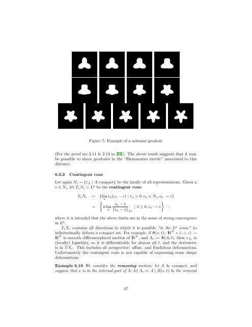
6.2.4 Applications in computer visionCharpiat et al. [9] propose an approximation method to compute len H (ξ) bymeans of a family of energies defined using a smooth integrand; the approximationis mainly based on the property ‖f‖ L p → p ‖f‖ L ∞, for any measurable functionf defined on a bounded domain; they successively devise a method to findapproximation of geodesics.6.3 A Hausdorff-like distance of compact setsIn Duci and Mennucci [15] a L p -like distance on the compact subsets of lR N wasproposed. (Here p ∈ [1, ∞).)To this end, we fix ϕ : [0, ∞) → (0, ∞) , decreasing, C 1 , with ϕ(|x|) ∈ L p . Wethen define v A (x) := ϕ(u A (x)), where u A is the distance function. We eventuallydefine the distanced(A, B) := ‖v A − v B ‖ L p . (6.2)Remark 6.15 This shape space is a perfect example of the representation/embedding/quotient scheme. Indeed, this shape space is represented as N c ={v A | A compact} and embedded in L p . Given v ∈ N c , we recover the shapeA = {v = ϕ −1 (0)} (that is a level set of v).Example 6.16 A simple example (that works for all p) is given by ϕ(t) = e −t ,so that v A (x) = exp (−u A (x)); in this case, A = {v = 1}.The distance d of eqn. (6.2) enjoys the following properties.Properties 6.17• It is Euclidean invariant;• it is locally compact but not path-metric;• the topology induced is the same as that induced by d H ;• minimal geodesics do exist, since D g := {B | d g (A, B) ≤ ρ} is compact.The proofs are in [15]. We present a numerical computation of a minimal geodesic(by A. Duci) in Figure 7 on the next page.6.3.1 Analogy with the Hausdorff metric, L p vs L ∞We recall that d H (A, B) = ‖u A (x) − u B (x)‖ L ∞ ; whereas instead now we areproposing d(A, B) := ‖v A −v B ‖ L p . The idea being that this distance of compactsets is modeled on L p , whereas the Hausdorff distance is “modeled” on L ∞ .(Note that the Hausdorff distance is not really obtained by embedding, sinceu A ∉ L ∞ ). L p is more regular than L ∞ , as shown by this remark.Remark 6.18 Given any f, g ∈ L p with p ∈ (1, ∞), the segment connectingf to g is the unique minimal geodesic connecting them. Suppose now that thedimension of L ∞ (Ω, A, µ) is greater than 1. Given generically f, g ∈ L ∞ , thereis an uncountable number of minimal geodesics connecting them. 99 “Generically” is meant in the Baire sense: the set of exceptions is of first category.46
Figure 7: Example of a minimal geodesic(For the proof see 2.11 & 2.13 in [15]). The above result suggests that it maybe possible to shoot geodesics in the “Riemannian metric” associated to thisdistance.6.3.2 Contingent coneLet again N c = {v A | A compact} be the family of all representations. Given av ∈ N c , let T v N c ⊂ L p be the contingent coneT v N c := {lim t n (v n − v) | t n > 0, v n ∈ N c , v n → v}n{}v n − v= λ lim | λ ≥ 0, v n → v ,n ‖v n − v‖ L pwhere it is intended that the above limits are in the sense of strong convergencein L p .T v N c contains all directions in which it is possible “in the L p sense” toinfinitesimally deform a compact set. For example, if Φ(x, t) : lR N × (−ε, ε) →lR N is smooth diffeomorphical motion of lR N , and A t := Φ(A, t), then v At is(locally) Lipschitz, so it is differentiable for almost all t, and the derivativeis in T N c . This includes all perspective, affine, and Euclidean deformations.Unfortunately the contingent cone is not capable of expressing some shapedeformations.Example 6.19 We consider the removing motion; let A be compact, andsuppose that x is in the internal part of A; let A t := A \ B(x, t) be the removal47
- Page 1 and 2: Metrics of curves in shape optimiza
- Page 3 and 4: shape analysis where we study a fam
- Page 5 and 6: • F (c) = F (c ◦ φ) for all cu
- Page 7 and 8: κ > 0HNNHNHκ < 0Figure 1: Example
- Page 9 and 10: In the case of planar curves c 1 ,
- Page 11 and 12: (a) (b) (c) (d) (e)Figure 3: Segmen
- Page 13 and 14: where φ may be chosen to beφ(x) =
- Page 15 and 16: 2.4.1 Example: geometric heat flowW
- Page 17 and 18: 2.4.5 Centroid energyWe will now pr
- Page 20 and 21: shapes. Unfortunately, H 0 does not
- Page 22 and 23: • If the second request is waived
- Page 24 and 25: • The Fréchet space of smooth fu
- Page 26 and 27: Since φ k are homeomorphisms, then
- Page 28 and 29: 3.6.1 Riemann metric, lengthDefinit
- Page 30 and 31: Theorem 3.30 Suppose that M is a sm
- Page 32 and 33: Example 3.38 Let M = C ∞ ([−1,
- Page 34 and 35: • sometimes S 1 will be identifie
- Page 36 and 37: The proof is by direct computation.
- Page 38 and 39: The term preshape space is sometime
- Page 40 and 41: 5 Representation/embedding/quotient
- Page 42 and 43: 6.1.1 Length induced by a distanceI
- Page 44 and 45: 0101200000000000011111111111110000
- Page 48 and 49: of a small ball from A. The motion
- Page 50 and 51: CutΩ(The arrows represent the dist
- Page 52 and 53: 7.3 L 1 metric and Plateau problemI
- Page 54 and 55: Definition 8.3 (Flat curves) Let Z
- Page 56 and 57: Proof. Fix α 0 ∈ S \ Z. Let T =
- Page 58 and 59: 8.2.2 RepresentationThe Stiefel man
- Page 60 and 61: 9.3 Conformal metricsYezzi and Menn
- Page 62 and 63: 10.1.1 Related worksA family of met
- Page 64 and 65: Definition 10.7 (Convolution) A arc
- Page 66 and 67: and̂∇˜HjE(0) = ̂∇ H 0E(0),̂
- Page 68 and 69: and we simply integrate twice! More
- Page 70 and 71: Corollary 10.18 In particular, the
- Page 72 and 73: 10.6 Existence of gradient flowsWe
- Page 74 and 75: • The length functional (from C 1
- Page 76 and 77: We can eventually estimate the diff
- Page 78 and 79: 7.552.5-10 -7.5 -5 -2.5 2.5 5 7.5 1
- Page 80 and 81: By using (i) and (ii) from lemma 10
- Page 82 and 83: 10.6.3 Existence of flow for geodes
- Page 84 and 85: 10.7.1 Robustness w.r.to local mini
- Page 86 and 87: We already presented all the calcul
- Page 88 and 89: 10.9 New regularization methodsTypi
- Page 90 and 91: can be solved for k (this is not so
- Page 92 and 93: 2. Now• at t = 1/2 it achieves th
- Page 94 and 95: Definition 11.10 • The orbit is O
Figure 7: Example <strong>of</strong> a m<strong>in</strong>imal geodesic(For the pro<strong>of</strong> see 2.11 & 2.13 <strong>in</strong> [15]). The above result suggests that it maybe possible to shoot geodesics <strong>in</strong> the “Riemannian metric” associated to thisdistance.6.3.2 Cont<strong>in</strong>gent coneLet aga<strong>in</strong> N c = {v A | A compact} be the family <strong>of</strong> all representations. Given av ∈ N c , let T v N c ⊂ L p be the cont<strong>in</strong>gent coneT v N c := {lim t n (v n − v) | t n > 0, v n ∈ N c , v n → v}n{}v n − v= λ lim | λ ≥ 0, v n → v ,n ‖v n − v‖ L pwhere it is <strong>in</strong>tended that the above limits are <strong>in</strong> the sense <strong>of</strong> strong convergence<strong>in</strong> L p .T v N c conta<strong>in</strong>s all directions <strong>in</strong> which it is possible “<strong>in</strong> the L p sense” to<strong>in</strong>f<strong>in</strong>itesimally deform a compact set. For example, if Φ(x, t) : lR N × (−ε, ε) →lR N is smooth diffeomorphical motion <strong>of</strong> lR N , <strong>and</strong> A t := Φ(A, t), then v At is(locally) Lipschitz, so it is differentiable for almost all t, <strong>and</strong> the derivativeis <strong>in</strong> T N c . This <strong>in</strong>cludes all perspective, aff<strong>in</strong>e, <strong>and</strong> Euclidean deformations.Unfortunately the cont<strong>in</strong>gent cone is not capable <strong>of</strong> express<strong>in</strong>g some <strong>shape</strong>deformations.Example 6.19 We consider the remov<strong>in</strong>g motion; let A be compact, <strong>and</strong>suppose that x is <strong>in</strong> the <strong>in</strong>ternal part <strong>of</strong> A; let A t := A \ B(x, t) be the removal47


