Simplified models/procedures for estimation of ... - ELSA - Europa

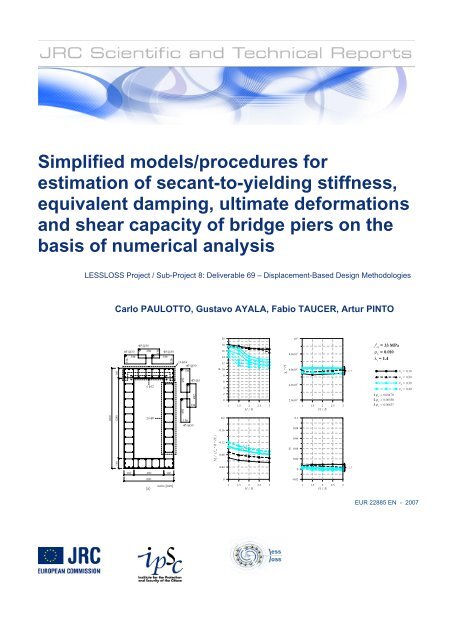
Simplified models/procedures forestimation of secant-to-yielding stiffness,equivalent damping, ultimate deformationsand shear capacity of bridge piers on thebasis of numerical analysisLESSLOSS Project / Sub-Project 8: Deliverable 69 – Displacement-Based Design MethodologiesCarlo PAULOTTO, Gustavo AYALA, Fabio TAUCER, Artur PINTO1600160 1280 160φ5 @50 330 φ5 @50136φ5 @506 φ1220 φ8136346 346136160 480 16014 φ14φ5 @50136492492492136136φ5 @50φ5 @50M y / ( f' cm * B * H 2 )µ201816141210864200.20.160.120.080.043213211, 2, 31 1.5 2 2.5 3H / B1, 2, 31, 2, 31, 2, 31, 2, 331,2χ y * Hα10 -28.0x10 -36.0x10 -34.0x10 -32.0x10 -30.10.080.060.040.0201 1.5 2 2.5 3H / B1, 2, 31, 2, 3f' cm= 33 MPaρ L= 0.010λ c= 1.41 ρ w = 0.004782 ρ w = 0.005583 ρ w = 0.00637ν k = 0.10ν k = 0.20ν k = 0.30ν k = 0.408000-0.02(a)units [mm]1 1.5 2 2.5 3H / B1 1.5 2 2.5 3H / BEUR 22885 EN - 2007

The Institute for the Protection and Security of the Citizen provides researchbased, systemsorientedsupport to EU policies so as to protect the citizen against economic and technologicalrisk. The Institute maintains and develops its expertise and networks in information,communication, space and engineering technologies in support of its mission. The strongcrossfertilisation between its nuclear and non-nuclear activities strengthens the expertise it canbring to the benefit of customers in both domains.European CommissionJoint Research CentreInstitute for the Protection and Security of the CitizenContact informationAddress: Fabio TAUCERE-mail: fabio.taucer@jrc.itTel.: +39 0332 78.5886Fax: +39 0332 78.9049http://ipsc.jrc.ec.europa.euhttp://www.jrc.ec.europa.euLegal NoticeNeither the European Commission nor any person acting on behalf of the Commission isresponsible for the use which might be made of this publication.A great deal of additional information on the European Union is available on the Internet.It can be accessed through the Europa serverhttp://europa.eu/JRC38009EUR 22885 ENISSN 1018-5593Luxembourg: Office for Official Publications of the European Communities© European Communities, 2007Reproduction is authorised provided the source is acknowledgedPrinted in Italy

Simplifiedmodels/proceduresfor estimation ofsecant-to-yieldingstiffness, equivalentdamping, ultimatedeformations andshear capacity ofbridge piers on thebasis of numericalanalysis

iEXECUTIVE SUMMARYCurrent seismic evaluation and design tendencies for reinforced concrete bridges, in whichperformances under design conditions need to be estimated, require, even in the most simplifiedmethods, an accurate description of the stiffness and energy dissipation characteristics of thepiers forming the substructure. This description involves not only the use of sound analyticaltechniques, but also their calibration against existing results from experimental tests on large scalespecimens.Considering that the most widely used approach for the Displacement Based Design of bridges isbased on the use of secant stiffness and equivalent viscous damping of the piers, both evaluatedat maximum pier displacement, in this report the stiffness and energy dissipation characteristics,necessary to estimate these parameters, are obtained for reinforced concrete hollow rectangularbridge piers. This work involves the use, first of a continuous non-linear behaviour section modeland then a pier model based on the plastic hinge approach and on the results obtained by thesection model of the previous step.The analysis starts from the identification of the parameters that play a major role in determiningthe behaviour of pier sections and their ranges of variation. The following parameters werechosen: the section aspect ratio, the mechanical properties of the reinforcement steel andconcrete, the longitudinal reinforcement ratio, the normalized axial force and the confinementlevel. The range of variation of each of these parameters was determined on the basis of currentpractice and the prescriptions contained in the Eurocodes. As a result of this preliminary analysis,2700 possible section designs were considered.To determine the moment-curvature envelope of all the sections considered, nonlinear finiteelement analyses (using a 2D fibre model) under monotonically increasing curvatures werecarried out. These capacity curves, representing the envelope curves of each section, areapproximated with bilinear curves to be used either for evaluation or design purposes. In thisway, the capacity curve of the generic section may be represented through four parameters: yieldcurvature and moment, and ultimate curvature and moment, which were used to summarize theresults in a series of charts. The cyclic behaviour of each section is reproduced through nonlinearanalysis under increasing cyclic loading, for which experimental results were also available. Theresults of these analyses were expressed in terms of a dimensionless parameter that is related tothe energy dissipated per unit length by the section in a cycle. It was found that this parameterdoes not depend on the section aspect ratio, while it depends strongly on the normalized axialforce, although this dependence becomes less strong as the longitudinal reinforcement ratioincreases.The properties derived at the section level are used to compute the force-displacement envelopeand the energy dissipation characteristics of a pier of length L for a given level of ductility of thesection; the calculations are performed assuming an expression derived from literature for thecomputation of the plastic length.The equivalent properties of bridge piers, namely, equivalent stiffness and equivalent damping atmaximum displacement, are calculated for rectangular hollow sections, and represent a significantdesign tool of direct application to the Displacement Based Design (DBD) of bridges, based onthe concept of a substitute linear structure as originally defined by Gulkan and Sozen in 1967.From the analysis of the experimental data it was observed that the shear contribution to the pierdisplacements can be significant. A state of art was produced concerning the differentapproaches that may be adopted to model the shear effects in reinforced concrete columns. Thefollowing models were analysed: the truss model, the classical Ritter-Morsch model, the concretecontribution model, the variable truss model, the strut and ties model, Compression Field Theory(CFT) and the Modified CFT (MCFT).

iiiTABLE OF CONTENTSLIST OF TABLES ....................................................................................................................................................... vLIST OF FIGURES................................................................................................................................................... viiLIST OF SYMBOLS AND ABBREVIATIONS................................................................................................... xi1. INTRODUCTION.................................................................................................................................................. 1PART A: STIFNESS AND ENERGY DISSIPATION EQUIVALENT PROPERTIES.............................. 22. SELECTION OF THE EXPERIMETAL DATA............................................................................................. 22.1 GENERALITIES................................................................................................................................................... 22.2 DESCRIPTION OF THE EXPERIMENTAL SET-UP AND RESULTS .................................................................. 32.2.1 Applied Horizontal Displacements..................................................................................................... 32.2.2 Applied Vertical Load........................................................................................................................... 42.2.3 Moment-Curvature Time-Histories .................................................................................................... 43. NUMERICAL MODEL ......................................................................................................................................... 53.1 GENERALITIES................................................................................................................................................... 53.2 STEEL AND CONCRETE MODELS .................................................................................................................... 53.2.1 Confined Concrete................................................................................................................................ 63.3 VALIDATION OF THE NUMERICAL MODEL.................................................................................................. 84. PARAMETRIC ANALYSIS OF THE SECTIONS .......................................................................................... 94.1 GENERALITIES................................................................................................................................................... 94.2 STEEL AND CONCRETE CHARACTERISTICS ................................................................................................... 94.3 WALL THICKNESS............................................................................................................................................ 104.4 SECTION ASPECT RATIO................................................................................................................................. 104.5 LONGITUDINAL REINFORCEMENT RATIO...................................................................................................104.6 AXIAL LOAD LEVEL........................................................................................................................................ 114.7 CONFINEMENT LEVEL.................................................................................................................................... 114.8 FAILURE CRITERIA OF THE SECTIONS..........................................................................................................134.9 IDEALIZED MOMENT-CURVATURE RELATIONSHIP...................................................................................145. RESULTS ON EQUIVALENT SECTION PROPERTIES: MOMENT-CURVATURE ANDENERGY DISSIPATION ....................................................................................................................................... 146. FROM SECTION TO MEMBER PROPERTIES ..........................................................................................15

ivPART B – SHEAR EFFECTS ON BRIDGE PIERS.......................................................................................... 197. SHEAR TESTS ON HOLLOW COLUMNS................................................................................................... 198. RITTER – MÖRSCH TRUSS MODEL ............................................................................................................ 209. TRUSS MODELS .................................................................................................................................................. 239.1 PRIESTLEY ET AL. [1994] ................................................................................................................................ 269.2 SEZEN AND MOEHLE [2004].......................................................................................................................... 279.3 STRUT-AND-TIE MODEL.................................................................................................................................. 2810. COMPRESSION FIELD THEORY (CFT).................................................................................................... 2910.1 COMPATIBILITY CONDITIONS.......................................................................................................................3010.2 EQUILIBRIUM CONDITIONS ..........................................................................................................................3010.3 STRESS-STRAIN RELATIONSHIP.....................................................................................................................3111. ANALYSIS OF RC MEMBERS SUBJECTED TO SHEAR, MOMENT AND AXIAL LOADUSING THE MCFT.................................................................................................................................................. 3412. DESIGN PROCEDURE BASED ON THE MCFT .................................................................................... 3613. CYCLIC LOAD MODELING THROUGH THE MCFT .......................................................................... 3713.1 PLASTIC OFFSET FORMULATION ..................................................................................................................3913.2 CONCRETE STRESS-STRAIN MODEL .............................................................................................................4113.2.1 Compression response........................................................................................................................ 4113.2.2 Tension response................................................................................................................................. 4313.2.3 Cracking-closing model ...................................................................................................................... 4413.3 REINFORCEMENT MODEL.............................................................................................................................4414. CONCLUSIONS ................................................................................................................................................. 45REFERENCES........................................................................................................................................................... 47TABLES....................................................................................................................................................................... 53FIGURES .................................................................................................................................................................... 59

vLIST OF TABLESTable 1 Mechanical properties of reinforcement steel (average values) 53Table 2 Mechanical properties of concrete (average values) 53Table 3 Values of the parameters of the model implemented in Castem2000 [Maillard, 1993] for confinedconcrete referred to the flanges of the section of the medium pier of bridge B232 53Table 4 Values of the parameters of the Mander’s model for the confined concrete. They refer to theconcrete in the flanges of the section of the medium pier of the bridge B232 54Table 5 Stress and deformation characteristics of concrete according to prEN 1992-1-1 [CEN, 2003]: f ckand f cm are the characteristic and mean values of the compressive strength, respectively; f ctm isthe mean value of the tensile strength and E cm is the mean value of the modulus of elasticity 54Table 6 Stress and deformation characteristics of steel reinforcement according to prEN 1998-2 E.2.2[CEN, 2003]: f yk and f ym are the characteristic and mean values of the yield stress,respectively. ε uk and ε um are the characteristic and mean values of elongation at maximumstrength, respectively 54Table 7 With reference to Figure 21, steel reinforcement diameter (mm) as a function of bar spacing i andrlongitudinal reinforcement ratio ρ L ; only bar diameters between 16mm and 32mm havebeen accepted. 54Table 8 Allowed distances (mm), in the horizontal plane, between two consecutive engaged rebars for thecase ν k ≤ 0.2 55Table 9 Allowed distance (mm), in the horizontal plane, between two consecutive engaged rebars for thecase ν k > 0.2 55Table 10 Allowed spacing (mm), along the vertical direction, for transverse reinforcement for the case ν k≤ 0.2 55Table 11 Allowed spacing (mm), along the vertical direction, for transverse reinforcement for the case ν k> 0.2 55Table 12 Values of the factor α n defined according to Equation (3.16) for the case ν k ≤ 0.2 55Table 13 Values of factor α s defined according to Equation (3.17) for the case ν k ≤ 0.2 56Table 14 Values of the confinement effectivness factor α evaluated according to Equation (3.15) for thecase ν k ≤ 0.2 56Table 15 Values of factor α n defined according to Equation (3.16) for the case ν k > 0.2 56Table 16 Values of factor α s defined according to Equation (3.17) for the case ν k > 0.2 56Table 17 Values of the confinement effectiveness factor α evaluated according to Equation (3.15) for thecase ν k > 0.2 56

viTable 18 Transverse reinforcement rebar sizes (mm) for the case ν k ≤ 0.2 57Table 19 Transverse reinforcement ratios for the case ν k ≤ 0.2 57Table 20 Coefficients of Equations (3.26) and (3.27), as given in Table 6.1 of prEN 1998-2 [CEN, 2003]. 57Table 21 Confinement pressure and confinement parameter for different shear reinforcement ratios andclasses of concrete 57Table 22 Values of the parameters considered in the parametric analysis 57Table 23 Values of θ and β for members containing at least the required minimum amount of stirrups 58

viiLIST OF FIGURESFigure 1 (a) Reinforcement layout of the pier section; (b) Geometric characteristics of the pier andinstrumentation placement 59Figure 2 Displacement and force time-history applied at the top of the pier in the horizontal directionduring the first PSD test (bridge subjected to the design earthquake) 59Figure 3 Displacement and force time-history applied at the top of the pier in the horizontal directionduring the second PSD test (bridge subjected to two time the design earthquake) 60Figure 4 Displacement and force time-history applied at the top of the pier in the horizontal directionduring the cyclic test 60Figure 5 Application of the vertical load to the pier: (a) post-tensioning method; (b) correct approachneeded for testing 60Figure 6 Moment-curvature plot of the response of the pier to the design earthquake at slice #1 61Figure 7 Moment-curvature plot of the response of the pier to two time the design earthquake at slice #1 61Figure 8 Moment-curvature plot of the response of the pier to the cyclic excitation at slice #1 62Figure 9 Concrete model for monotonic loading 62Figure 10 Concrete model for cyclic loading 62Figure 11 Comparison between Mander’s model and Castem 2000 [Maillard, 1993] model for theconfined concrete in the flanges of the section of the medium pier of bridge B232 63Figure 12 Comparison between the numerical and experimental results relative to slice #1 of the pierwhen subjected to the first few seconds of the design earthquake 63Figure 13 Comparison between the numerical and experimental results relative to slice #2 of the pierwhen subjected to the first few seconds of the design earthquake 63Figure 14 Comparison between the numerical and experimental results relative to slice #3 of the pierwhen subjected to the first few seconds of the design earthquake 64Figure 15 Comparison between the numerical and experimental results relative to slice #4 of the pierwhen subjected to the first few seconds of the design earthquake 64Figure 16 Comparison between the numerical and experimental results relative to slice #1 of the pierwhen subjected to the entire duration of the design earthquake 65Figure 17 Comparison between the numerical and experimental results relative to slice #2 of the pierwhen subjected to the entire duration of the design earthquake 65Figure 18 Comparison between the numerical and experimental results relative to slice #3 of the pierwhen subjected to the entire duration of the design earthquake 65Figure 19 Comparison between the numerical and experimental results relative to slice #4 of the pierwhen subjected to the entire duration of the design earthquake 66

viiiFigure 20 Comparison between the energy dissipated per cycle by the numerical model and by thesections belonging to different pier slices for cyclic tests of increasing amplitude 66Figure 21 Typical section of the bridge pier wall considered in the parametric analysis 66Figure 22 Plot of Equation (3.27) which gives the minimum amount of confining transversereinforcement when ν k > 0.20. The white dots represent the minimum amount oftransverse reinforcement against buckling requested by prEN 1998-2 when ν k ≤ 0.20. It isevident that when ν k ≤ 0.20 the provisions against buckling are more stringent than theconfining provisions 67Figure 23 Evaluation of the range of transverse reinforcement ratio values ρ w corresponding to a givenvalue of the confinement parameter λ c 67Figure 24 Construction of the bilinear approximation of the nonlinear skeleton curve of the pier sectionbehaviour 67Figure 25 Bilinear skeleton curves corresponding to sections characterized by different aspect ratios(section depth and width are expressed in m) and different longitudinal reinforcementratios. The remaining parameters are common to all the sections: concrete C25, ν k = 0.60,λ c = 1.4 68Figure 26 Bilinear skeleton curves corresponding to sections characterized by different aspect ratios(section depth and width are expressed in m) and different longitudinal reinforcementratios. The remaining parameters are common to all the sections: concrete C25, ν k = 0.10,λ c = 1.4 68Figure 27 Results of the parametric analysis (f’ cm = 33 MPa, ρ L = 0.005, λ c = 1.0) 69Figure 28 Results of the parametric analysis (f’ cm = 33 MPa, ρ L = 0.005, λ c = 1.2) 69Figure 29 Results of the parametric analysis (f’ cm = 33 MPa, ρ L = 0.005, λ c = 1.4) 70Figure 30 Results of the parametric analysis (f’ cm = 33 MPa, ρ L = 0.005, λ c = 1.6) 70Figure 31 Results of the parametric analysis (f’ cm = 33 MPa, ρ L = 0.005, λ c = 1.8) 71Figure 32 Results of the parametric analysis (f’ cm = 33 MPa, ρ L = 0.005, λ c = 2.0) 71Figure 33 Results of the parametric analysis (f’ cm = 33 MPa, ρ L = 0.010, λ c = 1.0) 72Figure 34 Results of the parametric analysis (f’ cm = 33 MPa, ρ L = 0.010, λ c = 1.2) 72Figure 35 Results of the parametric analysis (f’ cm = 33 MPa, ρ L = 0.010, λ c = 1.4) 73Figure 36 Results of the parametric analysis (f’ cm = 33 MPa, ρ L = 0.010, λ c = 1.6) 73Figure 37 Results of the parametric analysis (f’ cm = 33 MPa, ρ L = 0.010, λ c = 1.8) 74Figure 38 Results of the parametric analysis (f’ cm = 33 MPa, ρ L = 0.010, λ c = 2.0) 74Figure 39 Results of the parametric analysis (f’ cm = 33 MPa, ρ L = 0.020, λ c = 1.2) 75Figure 40 Results of the parametric analysis (f’ cm = 33 MPa, ρ L = 0.020, λ c = 1.4) 76Figure 41 Results of the parametric analysis (f’ cm = 33 MPa, ρ L = 0.020, λ c = 1.6) 76

xFigure 68 Average stress-strain relationship for cracked concrete in compression 89Figure 69 Average stress-strain relationship for cracked concrete in tension 89Figure 70 (a) Calculated average stresses. (b) Local stresses at a crack 90Figure 71 Layered model of the member section 90Figure 72 Free-body diagram for concrete layer k 90Figure 73 Determination of strain ε x for a non-prestressed beam 91Figure 74 Hysteresis model for concrete in compression: unloading branch (from [Palermo and Vecchio,2003]) 91Figure 75 Hysteresis model for concrete in compression: reloading branch (from [Palermo and Vecchio,2003]) 91Figure 76 Hysteresis model for concrete in tension: unloading branch (from [Palermo and Vecchio,2003]) 92Figure 77 Hysteresis model for concrete in tension: reloading branch (from [Palermo and Vecchio, 2003]) 92

xiiiabb vd vd bf c1f c2f cxf cyf sxf sxcf syf sycrf vf vyf xf yf yxf yyPART B= Shear span (distance from maximum moment section to point ofinflection); maximum aggregate size= Width of the member; width of concrete layer= Effective web width taken as minimum web width within effective sheardepth d v= Effective shear depth taken as flexural lever arm which, for nonprestressedelement= Bar diameter= Principal tensile stress in concrete= Principal compressive stress in concrete= Stress in concrete in x-direction= Stress in concrete in y-direction= Average stress in x-reinforcement= Stress in x-reinforcement at crack location= Average stress in y-reinforcement= Stress in y-reinforcement at crack location= Tensile stress existing in the stirrups= Yielding stress of transverse reinforcement= x-direction axial stress; stress applied to element in x-direction= y-direction axial stress; stress applied to element in y-direction= Yield stress of x-reinforcement= Yield stress of y-reinforcementf’ c = Maximum compressive stress observed in a cylinder testhkss mxs mys θv civ cxv cxyv cyv sxv sy= Depth of concrete layer= Factor for shear strength of concrete shear resisting mechanism= Stirrup spacing= Indicator of the crack control characteristics of the x-reinforcement= Indicator of the crack control characteristics of the y-reinforcement= Diagonal crack spacing= Shear stress on crack surface= Shear stress on x-face of concrete= Shear stress on concrete relative to x,y axes= Shear stress on y-face of concrete= Shear stress on x-reinforcement= Shear stress on y-reinforcement

xivν xywxyyA gA hA vCC sD= Shear stress; shear stress on element relative to x, y-axis= Crack width= Distance from the column axis perpendicular to the applied shear force= Distance from top of beam section= Distance from top to centroid of section= Gross area of the member section= Area of one hoop leg= Total area of transverse reinforcement in the shear direction within adistance s= Compressive force acting on layer face= Compressive force acting in longitudinal bar= Diameter of a circular columnD’ = Diameter of a spiral hoopE cE cE sE sFMNPSVV cV sαγ xy= Young’s modulus of concrete= Secant modulus of concrete= Young’s modulus of reinforcement= Secant modulus of reinforcement= Force= Moment acting on member section= Axial force acting on member section= Axial load= Spacing between member cross sections= Shear resistance; shear force acting on a member section= Concrete contribution to the shear resistance= Transverse reinforcement contribution to the shear resistance= Angle between tangent to spiral and direction of shear force; angle formedbetween the column axis and the strut from the point of load application tothe centre of the flexural compression zone at the column plastic hingecritical section; reinforcement orientation= Shear strain relative to x,y-axispγ cxy = Plastic shear strain in concrete relative to x, y-axesεε beε cpε cε t= Instantaneous strain in concrete= Bottom fibre strain in beam sections= Elastic strain of concrete= Residual (plastic offset) strain of concrete= Top fibre strain in beam sections

xvε xε yε 1= Strain in x-direction= Strain in y-direction= First principal strain in concrete

11. INTRODUCTIONA number of important bridges and viaducts which incorporate reinforced concrete thin-walledhollow piers have been constructed during the past decades in seismic prone regions. The mainadvantage of this type of piers is that their mass is significantly smaller than that of piers withsolid column sections of equivalent performance, thus reducing the amount of material used anddecreasing the size of the inertial forces induced by earthquake loads. In spite of the morecomplex reinforcement layout and formwork construction, hollow columns are considered, ingeneral, to be cost effective for large scale projects and for pier heights exceeding 20 m.In spite of the use of hollow column sections for the construction of large bridge piers, theirbehaviour has not been extensively studied; in particular, a limited number of experimental testshave been performed to describe the load-deformation and energy dissipation characteristics ofsuch members. The aim of this report is to describe these characteristics for different levels ofdeformation to be used within the context of Performance Based Design (PBD).The report is subdivided in two parts: the first part (Part A) describes the moment-curvaturerelations and the energy dissipation characteristics of rectangular pier hollow sections of variousdesign configurations, and the second part (Part B) describes the shear effects on reinforcedconcrete bridge piers.In Part A, the stiffness and energy dissipation characteristics of the pier are derived based onenergy principles from the section properties at the base of the pier. The stiffness properties ofthe section are described by a bilinear moment-curvature model defined by the bending momentsand curvatures at yield and at the ultimate capacity of the section, derived from nonlinear analysisusing a 2D fibre model initially calibrated from experimental results. The energy dissipationcharacteristics of the section are derived directly from the numerical model at increasing levels ofductility. Parametric analysis is performed for a large number of design configurations of the piersection, including the aspect ratio of the section, the normalised axial load, the percentage oflongitudinal reinforcement, the level of confinement, and the strength of concrete and steel, andthe results are summarised in series of charts that can be used by the designer to defined themoment-curvature diagram (including stiffness to yield and maximum curvature capacity) for aparticular section. Similarly, a number of charts are presented, describing the energy dissipationfor several section configurations for different levels of ductility.In Part B, the state-of-the-art on the different approaches to model the effects of shear onreinforced concrete column sections is presented, starting from the truss model, that considersonly the contribution of the steel stirrups, up to the modified compression field theory, that takesinto account the three dimensional contribution along the section of both shear and bending.The theoretical explanation is supported by experimental tests performed on reinforced concretehollow sections considering shear, as well as on walls that may be approximated to the webs ofthe pier. However, there is a need to extend the more detailed models to cyclic loading and toperform target tests on large scale piers to model the combined effects of shear and flexure.

2PART A: STIFNESS AND ENERGY DISSIPATIONEQUIVALENT PROPERTIES2. SELECTION OF THE EXPERIMETAL DATA2.1 GENERALITIESThe numerical models used in this research were calibrated against the results of experimentaltests conducted on large-scale models of hollow reinforced concrete piers at the EuropeanLaboratory for Structural Assessment (ELSA) in Ispra (Italy) [Pinto et al., 1996]. Theseexperimental models used in the tests were chosen with the aim to reduce as much as possiblethe consequences of the scale effect in the calibration process.Only a few number of documents are found in the technical literature focused on the scale effecton experimental tests of reinforced concrete bridge piers: [Stone and Cheok, 1989], [Hoshikumaet al., 2002] and [Yeh et al., 2002]. Stone and Cheok [1989] conducted a series of cyclic loadingtests on full-scale circular columns, with a diameter of 1524 mm, and their relative well-scaledreplica model, to determine the size effect on inelastic behaviour of reinforced concrete columnssubjected to seismic forces. They found that the scale effect does not appear when reinforcementdetails including bar diameter and vertical hoop spacing are precisely scaled.Hoshikuma et al. [2002] tested a full-scale column with a 2400 mm square section and a 1/4 scalereplica model. The columns were subjected to a quasi-static, cyclically reversed horizontal loaduntil the columns were completely failed. No vertical loads were applied to the prototype nor tothe model. As Stone and Cheok [1989], they concluded that if the reinforcement details areprecisely scaled, the size effect on the inelastic ductile behaviour of reinforced concrete bridgecolumns is not significant.Yeh et al. [2002] carried out experimental tests on square hollow reinforced concrete bridgecolumns. Two prototypes and four models of such columns were tested under constant axialloads and quasi-static, cyclically reversed horizontal loads. The prototype cross sections were1500 x 1500 mm and the scale factor of the models was equal to 1/3. Yeh et al. [2002] found thatthe prototypes have greater ductility factors than those given by the models and pointed out twopossible sources for this discrepancy: a difference in the yielding characteristics between therebars used as longitudinal reinforcement in the prototypes and those used in the models, and theeffect of low-cycle fatigue, which has a stronger influence on the small size rebars used in themodels. However, it should be noted that the scaling criteria applied by Stone and Cheok [1989]and in Hoshikuma et al. [2002] were not completely satisfied by Yeh et al. [2002]. It is opinion ofthe author that this could be the reason for the strong scale effect observed by Yeh et al. [2002],since differences in the yielding characteristics of the reinforcement and low-cycle fatigue affectswere also present in Stone and Cheok [1989] and in the Hoshikuma et al. [2002] tests.

3On the basis of these results, it can be concluded that the models tested by Pinto et al. [1996] canreasonably represent the actual behaviour of hollow reinforced concrete bridge piers, since theysatisfy the scaling criteria applied by Stone and Cheok [1989] and Hoshikuma et al. [2002]. In fact,Pinto et al. [1996] used rebars with diameters ranging between 10 mm and 14 mm as longitudinalreinforcement in the flanges of the models (according to Mander [1984], the flange wallsdetermine the behaviour of hollow rectangular concrete piers). Considering that the model scalefactor was 1:2.5, these rebars correspond to prototype rebars having diameters in the range of 25-35 mm, which are commonly used in current practice for this type of structures. Analogousconsiderations can be made for the size of transverse reinforcement (5 mm for the models and12.5 mm for the prototypes) and spacing of transverse reinforcement along the pier (50 mm forthe models and 125 mm in the prototypes). If a criticism can be made on these models, is thatthe longitudinal reinforcement is not uniformly distributed on the section, as generally happens incurrent practice.2.2 DESCRIPTION OF THE EXPERIMENTAL SET-UP AND RESULTSThe experimental tests preformed by Pinto et al. [1996] consisted in testing single piers subjectedto cyclic loading, as well as testing of a complete bridge structure by means of the pseudodynamic(PSD) sub-structured test method, which integrates physical testing of the pier modelsfor which the load-displacement behaviour is to be determined, with numerical models of thoseparts of the bridge for which the force-displacement response is known or remains elastic (i.e.,the deck). Several bridge configurations composed of three piers were studied, according to theirdegree of irregularity in terms of the heights and capacities of the piers. The results obtainedfrom the medium pier of the bridge B232 configuration were used for the calibration of thenumerical model.The geometric characteristics and the reinforcing steel lay-out of the pier model are presented inFigure 1. In order to determine the mechanical characteristics of concrete and steel, a set ofspecimens from the construction of the model were tested. The mechanical characteristics ofconcrete and steel reinforcement (Tempcore B500B) are reported in Table 1 and Table 2.The footing of the pier was rigidly attached to the strong floor of the laboratory by means ofpost-tensioned steel bars passing through the floor. The footing was prestressed in order to limitcracking when developing the maximum strength at the base of the pier.A stiff steel cap was connected with bolts and epoxy resin to the top of the pier (see Figure 1b).The cap was used to apply the horizontal loads coming from the PSD test method, and toimpose the vertical loads needed to simulate the weight of the bridge superstructure.2.2.1 Applied Horizontal DisplacementsTwo actuators were connected by spherical joints to the steel cap of the pier, on one side, and toa steel plate attached to the reaction wall on the opposite side, and were used to imposehorizontal displacements. The pier was tested as part of a bridge configuration for twoconsecutive earthquakes using the PSD technique. The first earthquake, hereafter denoted as“design earthquake”, was a stationary artificial earthquake with a PGA of 0.35g compatible withthe prEN 1998-2 [CEN, 1993] spectrum for soil type B. The second earthquake was obtained bymultiplying the ordinates of the first one by a factor 2. In Figure 2 and Figure 3 are reported thedisplacement and force time-histories measured at the top of the considered pier during thesetwo tests. Finally, the pier was isolated from the bridge model and tested cyclically until failure.Figure 4 illustrates the displacement and force time-histories applied at the top of the pier duringthe cyclic test.

42.2.2 Applied Vertical LoadA vertical force of 1700 kN, corresponding to a 10% normalized axial force, was applied at thetop of the pier and was kept practically constant during the whole duration of the test. Thevertical load was applied by means of four actuators resting on top of the steel cap and hingedconnected to post-tensioning steel rods running through the hollow core of the pier section; thesteel rods were embedded at the base of the pier footing and instrumented with strain gages tomonitor the axial load. The direction of the axial force follows the direction of post-tensioning(see Figure 5a) and can be decomposed into a horizontal (P·sin α) and a vertical component(P·cos α), so that the moment M at the column interface with the footing can be evaluated as:M = V ⋅ L+ P′⋅Δ= V ⋅ L+ P⋅cosα⋅Δ (2.1)while the total lateral force applied to the column is:V ′ = V − P ⋅ sinα(2.2)When a horizontal displacement history is applied to the pier, the gravity loads of the deck keepon acting along the vertical direction while the structure undergoes deformations (see Figure 5b).For this reason, Dutta et al. [1999] concluded that the post-tensioning method does not correctlymodel the P-∆ effect. Nevertheless, as noted by Asadollah and Xiao [2002], it can be asserted thatthe conventional method of post-tensioning is valid without any deficiency as long as the trueforces P' and V' are used in the data analysis. It is worth noting that α is typically small: duringthe cyclic test it attained a maximum value of about 0.03 rad, as a result P’ can be assumed to beequal to P.2.2.3 Moment-Curvature Time-HistoriesThe evaluation of the moment-curvature behaviour along the column was carried out on thebasis of the data given by a set of displacements transducers (LVDT) placed along the twoexternal opposite faces of the pier model. (See Figure 1b). The average curvature in a slice can beexpressed as:Δ − Δχ =D⋅lvi , v,jwhere χ is the average curvature over the considered slice, Δ vi and Δ vj are the relative verticaldisplacements measured by two transducers at the same height on the two sides of the pier, D isthe distance in plan between the two transducers and l is the height of the slice. Thecorresponding moment is calculated at the middle height of the slice, using the recorded valuesfor the horizontal force and axial load and the relative horizontal deflection at the correspondingstep.Figure 6 and Figure 7 show the moment-curvature responses of slice #1 (at the base of the pier)of the medium pier of bridge B232 subjected to the design earthquake and to the designearthquake multiplied by a factor of two, respectively. Figure 8 shows the analogous response ofthe pier tested under increasing cyclic displacements until failure.(2.3)

53. NUMERICAL MODEL3.1 GENERALITIESWith the purpose of simulating the behaviour of pier sections with characteristics different fromthose in the laboratory, a fibre model was implemented in Castem 2000 [Maillard, 1993] andchecked against the experimental results described in Section 0.Four different material models: reinforcement steel in the longitudinal direction, unconfinedconcrete, flange confined concrete and web confined concrete, were used to build the sectionmodel.3.2 STEEL AND CONCRETE MODELSThe monotonic behaviour of the steel fibre is represented by a three-stage stress-strain curve:linear elastic followed by a yielding plateau and a hardening zone modelled with a fourth degreepolynomial. The model for cyclic loading follows the monotonic curve until the strain falls belowa pre-established level after unloading from a postyielding position. From this point on, thestress-strain curve follows the Menegotto-Pinto [1973] model.The rebar buckling is modelled after Monti and Nuti [1992]. This model, which neglects theinfluence of concrete and transverse reinforcement, was calibrated against experimental testsconducted on Italian reinforcing rebars FeB 44k characterized by a more pronounced hardeningwhen compared with that shown by the modern Tempcore B500B rebars. This difference impliesthat Tempcore B500B bars are more prone to inelastic buckling than the FeB 44k rebars. For thisreason, a recalibration of the model, which at present has not been performed, would have beendesirable.The values reported in Table 1 were assigned to the parameters of the steel model. The ultimatetensile strain was reduced by 30%, recognizing that under cyclic loading involving sequentialtensile and compressive strains, the ultimate tensile strain is in general smaller than that obtainedfrom monotonic testing [Priesley et al. 1996b]. The onset of strain hardening was assumed at astrain equal to 2%.The Hognestad [1951] model was adopted for the concrete under monotonic compressiveloading. A parabolic function defines the ascending part of the curve from zero to the maximumcompression stress point. A straight line represents the concrete softening behaviour aftermaximum strength until failure. The slope of this line depends on the degree of confinement ofconcrete (see Figure 9). In order to improve the model for confined concrete, a third branch isconsidered after the softening compression branch and before reaching failure: a zero slopestraight line defining a compression plateau. This additional condition accounts for the residualstrength of the concrete core for important axial post-peak deformations. Following therecommendations of Park et al. [1982], a residual strength equal to 20% of the peak strength wasassumed in the model.The compression monotonic curve models the envelope of the behaviour of concrete undercompression cyclic loading. Unloading from the envelope follows a law similar to the oneproposed by Mercer and Martin [1987]: a straight line with a slope that depends on the maximum

6strain reached during the loading history (see Figure 10). The degradation of the material stiffnessis taken into account by decreasing the slope of the unloading branch as the maximum strainincreases. The reloading compression curve is also a straight line from the zero stress point to thelast loading point reached on the envelope; no strength degradation is considered.A bilinear model was used to represent the behaviour of concrete under monotonic tensileloading: a first linear branch with a slope equal to the initial compression Young’s modulus, fromzero to the maximum tensile stress point, and a second linear branch from the maximum tensilestress point to a zero stress point (see Figure 10); the post-cracking softening behaviour modelsthe “tension-stiffening” effect. Details on the model for cyclic tensile loading can be found inGuedes et al. [1994].No attempt was made to simulate the crack closing, since no reliable model has beenimplemented in Castem 2000 [Maillard, 1993] yet. As a result, the numerical model is expected toshow more pinching than the actual behaviour of the pier-section.3.2.1 Confined ConcreteThe behaviour of the confined concrete in the flanges of the pier section plays a major role indetermining the seismic performance of the pier. For this reason, special effort has been devotedto model its behaviour. Many different stress-strain relationships have been developed forconfined concrete: Sheik et al. [1982], Fafitis and Shah [1985], Mander et al. [1988], Saatcioglu andRazvi [1992], Sakino et al. [1993]. Among the aforementioned models, that proposed by Manderet al. [1988] is the only one that can be applied to all section shapes at all levels of confinement,furthermore it has also been accepted in prEN1998-2 [CEN, 2003], Annex E.Unfortunately, the model proposed by Mander et al. [1998] is not implemented in Castem 2000[Maillard, 1993]. As a result, an effort was made to evaluate the differences between the twomodels.In Castem 2000 [Maillard, 1993] the confinement effect is modelled through the confinementparameter β, which affects the strength, the strain at the maximum strength and the slope of thepost peak branch, as shown in the Equations (3.1), (3.2) and (3.3)fε= β ⋅fc , c c(3.1)2c1,c β ⋅εc1= (3.2)β − 0.85Z =β ⋅ ⋅α ⋅ ω + + ε( 0.1 w 0.0035 c,c)where f c,c and ε c1,c represent the maximum strength and the strain at the maximum strength forconfined concrete, while f c and ε c1 represent the analogous parameters for unconfined concrete; Zis the slope of the post peak branch (see Figure 9). The parameter β is defined as:where( )(3.3)β = min 1+ 2.5 ⋅α⋅ ω ,1.125 + 1.25 ⋅α⋅ω(3.4)ww∑( )Ast ⋅ f yw ⋅ lwsωw=b ⋅h ⋅ f0 0crepresents the mechanical volumetric ratio of the stirrups and(3.5)

7⎛ 8 ⎞ ⎛ s ⎞ ⎛ s ⎞α = ⎜1− ⎟⋅⎜1− ⎟⋅⎜1−⎟⎝ 3⋅n⎠ ⎝ 2⋅b0 ⎠ ⎝ 2⋅h0⎠(3.6)expresses the effect of the number of longitudinal restrained rebars n and the density of thestirrups on the degree of confinement of the concrete core. In Equations (3.5) and (3.6) A st , f ywand l w represent the area of the cross-section of the leg, the yielding stress and the total length ofthe stirrups, respectively; s is the distance between stirrups along the member axis, and b 0 and h 0are the dimensions of the confined concrete core measured from the centre-line of the stirrups.In Mander et al. [1998], the behaviour of the confined concrete is represented through acontinuous equation:σ c x ⋅r=f r −1+xc , cr(3.7)wherexc= (3.8)εεc1,cEr = (3.9)E −EsecccE secf c , c= (3.10)εc1,cThe confinement is taken into account by the confinement parameter λ c :σ e 2 ⋅σeλ c = 2.254⋅ 1 + 7.94 ⋅ − − 1.254(3.11)f fccwhich directly affects the maximum concrete strength and the corresponding strain:fελc , c = f c ⋅ c(3.12)⎡c,cc1, c = 0.002 ⋅ ⎢1+ 5⋅⎜−1fc⎣⎛⎝f⎞⎤⎟⎥⎠⎦(3.13)The confinement parameter λ c is a function of the effective confinement pressure:σ = α⋅ρ⋅ f(3.14)e w ywwhere:α = α n ⋅α s(3.15)biα n = 1 − ∑(3.16)6 ⋅ b ⋅ hn020⎛ s ⎞ ⎛ s ⎞α ⎜⎟ ⋅⎜ −⎟s = 1 − 1(3.17)⎝ 2 ⋅ b0 ⎠ ⎝ 2 ⋅ h0⎠

8Aswρ w =s ⋅ b(3.18)where b i is the distance between consecutive engaged bars, A sw is the total area of hoops or ties inthe direction of confinement and b is the dimension of the concrete core perpendicular to thedirection of the confinement under consideration, measured to the outside of the perimeterhoop.For rectangular sections, the confinement effects should be evaluated in two orthogonaldirections, say directions 2 and 3. When the values of ρ w in these two directions are not equal, theeffective confining stress may be estimated as:σ e = σe2 ⋅σe3 (3.19)The Mander et al. [1998] and the Castem 2000 [Maillard, 1993] models were compared for theconfined concrete of the flanges of the medium pier of bridge B232. The parameters of the twomodels corresponding to this case are reported in Table 3 and Table 4. Figure 11 shows theresults given by the two models. It can be seen that the two models give different values for themaximum concrete strength, with large differences in the softening branch. The results given bythe Castem 2000 [Maillard, 1993] model has been in part improved by equating the maximumconcrete strength given by the two models. The value of the parameter β is set equal to the valueof the λ c parameter in Mander’s model and the corresponding value of the product α·ω w isdetermined through Equation (3.19). The results are shown in Figure 11.3.3 VALIDATION OF THE NUMERICAL MODELIn order to judge the ability of the numerical model to represent the actual behaviour of piersections, the numerical results were compared with those obtained by the tests described inSection 0.The comparison was first focused on the initial stiffness of the sections. With this aim, the resultsrelative to the initial part of the design earthquake were considered. The results of thecomparison are shown in Figure 12, Figure 13, Figure 14 and Figure 15, for slice #1, #2, #3 and#4, respectively. It can be observed that the cracked stiffness of the section is well predicted forall the four pier slices considered in the analysis. The uncracked stiffness is well predicted forslices #3 and #4, while for slice #2, it was not possible to derive any considerations as theexperimental data was affected by noise. For slice #1 the initial stiffness is equal to the crackedstiffness, showing that this portion of the pier was already cracked at the beginning of the test.This was probably due to the presence of a cold joint between the plinth and the pier. In fact, thepier was made in a precast concrete workshop and then transported to the ELSA site where theplinth was cast in a separate phase.Finally, the ability of the numerical model to predict the section behaviour after the yielding pointwas checked. With this aim, the numerical results were compared with the experimental oneswhich had been obtained applying the design earthquake to the bridge model. The results areshown from Figure 16 to Figure 19. From these results, it is evident that the numerical model isable to follow the skeleton curve of the section. Furthermore, it can be observed that thebehaviour predicted by the numerical model is characterized by a very pronounced pinching thatis not exhibited by the experimental results. This discrepancy, as previously mentioned, is due tothe lack of a good crack opening-closure law in the numerical model.On the basis of the comparison between the numerical and the experimental results relative tothe design earthquake, it is concluded that the considered numerical model can be reasonablyused to obtain the skeleton curve of the behaviour of a generic rectangular hollow section. It is

9less clear if the numerical model is able to represent the hysteretic energy dissipated by sectionsdue to a more pronounced pinching of the numerical model. With the aim of clarifying thispoint, a cyclic path of curvatures with increasing amplitude was applied to the numerical modeland the results were compared with those obtained experimentally from the cyclic test describedin Section 2.2. From Figure 20 it can be observed that the numerical model gives a rather goodestimation of the energy dissipated by the section, at least in the case of cyclic tests. It should benoticed that overall, the different curvature paths used for the experimental and numerical testsseem not to affect the results.4. PARAMETRIC ANALYSIS OF THE SECTIONS4.1 GENERALITIESThe aim of this parametric analysis is to evaluate the moment-curvature behaviour of bridge piersections within the framework of Displacement Based Design (DBD) according to theprescriptions prEN 1998 [CEN, 2003].The analysis started from the identification of the parameters that play a major role indetermining the behaviour of the section. The parameters that were considered are: the concreteclass and the steel reinforcement yield strength, the wall thickness, the section aspect ratio, thelongitudinal reinforcement ratio, the axial load level, and the confinement level.The definition of the range of variation for each of these parameters is discussed in Sections 4.2to 4.7, while the values that were considered in the analysis are reported in Table 22. For each ofthe 2700 combinations of these values, two nonlinear static analyses, one monotonic, and onecyclic, were performed in order to obtain the skeleton curve and the damping properties of thecorresponding pier section. Finally, each skeleton curve was approximated through a bilinearcurve.4.2 STEEL AND CONCRETE CHARACTERISTICSAccording to prEN 1998-1 5.3.2 (1)P [CEN, 2003], class B or C steel reinforcement, as definedin Table C.1 in Normative Annex C of prEN 1992-1-1 [CEN, 2003], should be used in primaryseismic elements. Tempcore B500B reinforcing steel, which belongs to class B as defined byNormative Annex C, was considered in the analysis, with the following assumptions: steel tensilestrength f t equal to 1.19⋅f y [Priestley et al., 1996b]; elongation at maximum force ε u and strain atthe beginning of hardening equal to 0.11 and 0.02, respectively.According to prEN 1998-1 7.2.1 (1) [CEN, 2003], the prescribed concrete class in plastic regionsshould not be lower than C20/25, and not higher than C40/50. In the parametric analysis,concrete classes C25, C30 and C35 were considered.According to prEN 1998-1 4.3.3.4 (4) [CEN, 2003], the element properties should be based onthe mean values of the material properties. For new structures, the mean values of the materialproperties may be estimated from the corresponding characteristic values on the basis ofinformation provided in Annex E of prEN 1998-2 [CEN, 2003] and Table 3.1 of prEN 1992-1-1[CEN, 2003] (see Table 5 and Table 6) for the values assumed in the parametric analysis). Thisprovision recognizes the difference between designing for gravity loads and for earthquake

10actions. In the case of gravity load design, it is important to have an adequate reserve of strengthin order to avoid structural failure: the member properties are derived from a lower percentile ofmaterial properties (characteristic values). On the contrary, in the case of seismic design,structures are allowed to respond inelastically e.g., the action level overcomes the structuralstrength, therefore there is no point in providing for a reserve of strength.4.3 WALL THICKNESSFrom a survey of a number of bridge designs it was observed that the thickness of the walls thatconstitute the hollow sections varies between 0.30 m and 0.50 m. In the parametric analysis aconstant value of 0.40 m was chosen for the wall thickness.4.4 SECTION ASPECT RATIOPoston et al. [1985] conducted experimental tests on four bridge pier models. The objective ofthis work was to investigate the axial-load-moment-curvature behaviour of hollow columns andto examine the validity of the plane-section assumption. On the basis of their results and fromthose obtained by Proctor [1976, 1977] and Jobse [1982], Poston et al. [1985] concluded that theassumption is completely valid when the cross-sectional unsupported wall length to thicknessratio does not exceed 6. For ratios greater than 6, a strength reduction due to non-planar actionand local instability is recommended. Taylor and Breen [1994], on the basis of theaforementioned experimental results and from those obtained after testing twelve piers models,concluded that wall slenderness ratios greater than 35 should not be allowed in practice, and thatthe normal design procedure used to design solid piers should only be applied to hollow pierswhen the slenderness ratio is lower than 15. For wall slenderness ratios greater than 15, Taylorand Breen [1994] proposed a simplified design method that formed the basis for the provisionscontained in the AASHTO Specification [1998]. The validity of the results obtained by Taylorand Breen [1994] was confirmed by Santa Maria [2001], who tested five models of concretebridge piers. It is worth noting that all the previous tests where conducted monotonically andquasi-statically. Furthermore, only the effect of axial loads and bending moments wereconsidered in the analyses, with no reference to the effects of shear.According to prEN 1998-2 6.2.4 (2) [CEN, 2003], in plastic regions the wall slenderness ratioshould not exceed 8. Since in the parametric analysis the wall thickness was equal to 0.40 m, themaximum clear width of the wall is equal to 3.20 m. Furthermore, in the parametric analysis itwas considered a monocellular hollow pier with the outer dimension of the flange constant andequal to 2.00 m resulting in a section aspect ratio of 2.0 when the maximum wall slendernessratio allowed by prEN 1998-2 [CEN, 2003] is considered. In the parametric analysis aspect ratiovalues ranging between 1.0 and 3.0 have been considered, exceeding the maximum allowedslenderness ratio for aspect ratios larger than 2.4.5 LONGITUDINAL REINFORCEMENT RATIOThe longitudinal reinforcement ratio is defined as:Asρ L =Ac(3.20)where A s and A c are the total areas of longitudinal reinforcement and concrete cross-section.Lower and upper limits to longitudinal reinforcement ratio are usually specified by design codes.There is, however, an important variation in codified limits and in common design practiceamong different countries [Priestley et al., 1996b]. In the United States, it is permitted to vary the

11longitudinal reinforcement ratio for columns between 0.01 and 0.08. In New Zealand, thepermitted range is from 0.008 to 0.08. In Japan much lower reinforced ratios are permitted, andvalues as low as 0.005 are common. According to prEN 1998-1 5.4.3.2.2 (1) [CEN, 2003], thetotal longitudinal reinforcement ratio should not be less than 0.01 and not more than 0.04. Indesign practice, reinforcement ratios are usually between 0.01 and 0.03. In the present study,reinforcement ratios between 0.005 and 0.04 were considered, distributed in two layers ascommonly observed in practice. Furthermore, it was assumed that the reinforcement rebars,having all the same size, are uniformly distributed across the section.4.6 AXIAL LOAD LEVELThe normalized axial force is defined as:ν N Edk =A ⋅ f(3.21)cckwhere N ed is the axial force corresponding to the seismic design condition, A c is the area of theconcrete section and f ck is the characteristic value of concrete strength.According to prEN 1998-2 2.2.2.1 5(P) [CEN, 2003], plastic hinges shall not be formed inreinforced concrete sections where the normalized axial force exceeds 0.6. Furthermore, if thenormalized axial force is greater than 0.30, even in a single ductile member, the value of thebridge behaviour factor should be reduced (prEN 1998-2 4.1.6 5(P) [CEN, 2003]). As a result, indesign practice, normalized axial force values usually range between 0.10 and 0.30.4.7 CONFINEMENT LEVELThe confinement level of concrete in a section is related to the amount of transversereinforcement and its arrangement, which in turn is related to the amount and arrangement ofthe longitudinal reinforcement. The confinement level can be evaluated through Mander’sparameter λ c , as suggested by Annex E of prEN 1998-2 [CEN, 2003], using Equations from (3.7)to (3.19).In order to evaluate the range of variation of λ c , a 1.00 m section of a wall with a thickness of0.40 m was considered (see Figure 21). By assuming a value i for the distance between the centresof two consecutive rebars, the rebar size can be evaluated in terms of the longitudinalreinforcement ratio (see Table 7). It is reasonable to assume that the diameter of the longitudinalreinforcement of bridge piers may vary between φ16 mm and φ32 mm, so that any bar diameterresulting from the combination of the selected distance i and longitudinal reinforcement ratio ρ isdiscarded if it falls out of this range (see Table 7).For each spacing value i, the distance b i between two consecutive engaged rebars is evaluated.According to prEN 1998-2 6.2.4 (4) [CEN, 2003], if ν k ≤ 0.2 the requirements concerningbuckling of longitudinal compression reinforcement given in Section 6.2.2 need to be met;otherwise the confinement provisions given in Section 6.2.1 need to be met as well.According to prEN 1998-2 6.2.2 [CEN, 2003], longitudinal rebars should be restrained againstoutward buckling through: i) a perimeter tie engaged by intermediate cross-ties at alternatelocations of longitudinal bars at a horizontal spacing not exceeding 200mm (see Table 8); ii)transverse reinforcement at a vertical spacing not exceeding the value of the product between thediameter of the longitudinal rebars and factor δ (see Table 10), defined as:( ftkf yk )5≤ δ = 2.5⋅ + 2.25≤ 6(3.22)

12where f tk and f yk are the characteristic values of the tensile and yield strength of the transversereinforcement, respectively. Following Priestley et al. [1996b], a value equal to 1.19 has beenassumed for the ratio f tk /f yk , resulting in a value of δ equal to 5.According to prEN 1998-2 6.2.1 [CEN, 2003], the transverse distance between hoop legs orsupplementary cross-ties should not exceed 1/3 of the smallest dimension of the concrete core tothe hoop centreline, nor 200 mm (see Table 9) and the spacing of hoops or ties in the verticaldirection should be smaller than 6 times the longitudinal bar diameter and 1/5 of the smallestdimension of the concrete core measured to the hoop centreline.For each of the considered reinforcement arrangements, the values of the parameters α n , α s andα, defined according to Equations (3.16), (3.17) and (3.15), are evaluated. The results are shownin Table 12 and Table 17.According to prEN 1998-2 6.2.2 (4)P [CEN, 2003], if ν k ≤ 0.2, the minimum amount oftransverse ties is given by:min ⎜⎝ s⎛ At⎞ =T⎟⎠∑As⋅ f1.6 ⋅ fytys2(mm /m)(3.23)where A t is the area of one tie leg (in mm 2 ), s T is the vertical distance between tie legs (in m), ΣA sis the sum of the areas of the longitudinal bars restrained by the tie (in mm 2 ), f yt is the yieldstrength of the tie and f ys is the yield strength of the longitudinal reinforcement. From Equation(3.23), A t and the relative transverse reinforcement ratio can be determined for each consideredcouple of A s and s T values (see Table 18 and Table 19).For ν k > 0.2, both prEN 1998-2 6.2.1 (provisions against buckling) and 6.2.2 (confinementprovisions) [CEN, 2003] should be met. The quantity of confining reinforcement is definedthrough the mechanical reinforcement ratio:ω= ρ ⋅ f f(3.24)wd w yd cdwhere ρ w is the transverse reinforcement ratio defined as:Aswρ w =s ⋅bL(3.25)where A sw is the total area of hoops or ties in one direction of confinement; s L is the spacing ofhoops or ties in the vertical direction, b is the dimension of the concrete core perpendicular tothe direction of confinement under consideration, measured outside of the perimeter hoop.The minimum amount of confining reinforcement is determined, for rectangular hoops and crossties, as follows:⎛ 2 ⎞ωwd , r ≥ max ⎜ωw, req , ωw,min⎟⎝ 3 ⎠where:(3.26)Afcydωwreq = ⋅λ⋅ νk+ ⋅ ⋅( ρL−),A0.13 f0.01 (3.27)cccd

13where A c is the concrete gross section area; A cc is the confined concrete area of the section to thehoop centreline, ω w,min and λ are factors specified in Table 20 and ρ L is the reinforcement ratio ofthe longitudinal reinforcement. From Figure 22 it is possible to observe that the plot of Equation(3.27) in the ν k -ρ L -ω wd,r space is represented by a plane with a slope that depends on the values ofthe parameter λ given in Table 20. Figure 22 also shows the maximum transverse reinforcementratio 0.016 (ω wd,r = 0.346) needed to achieve a ductile seismic behaviour when ν k = 0.60 and ρ L =0.04.It can be concluded then that the transverse reinforcement ratios range between a minimum of0.003, obtained for ν k ≤ 0.20 and a low amount of longitudinal reinforcement (see Table 19), anda maximum ratio of 0.016. Assuming that the transverse reinforcement ratio is the same in bothdirections, orthogonal and parallel to the wall of Figure 21, the range of values of theconfinement pressure σ e and of the confinement parameter λ c can be evaluated throughEquations (3.14) and (3.11), respectively. The results are reported in Table 21.In the parametric analysis, λ c ranges between 0.0 and 2.0. For the concrete classes given in Table5 and the λ c values considered in the parametric analysis, the corresponding values of σ e areevaluated (see Figure 23) as a function of the transverse reinforcement ratio ρ w. The limits of thisrange correspond to the minimum and maximum values attained by the confinementeffectiveness parameter α (from about 0.6 to about 0.8) (see Table 14 and Table 17).4.8 FAILURE CRITERIA OF THE SECTIONSFailure of the reinforced concrete section is achieved when one of the following conditionsoccurs: i) the reinforcing steel attains its ultimate tensile strain; ii) the confined concrete reachesits ultimate compressive strain.In design and analysis of members subjected to earthquake loads, a reduced effective ultimatetensile strain should be adopted, since there is evidence that under cyclic loading involvingsequential tensile and compressive strains, the ultimate tensile strain is less than that obtainedunder monotonic testing [Priestley et al., 1996b]. The requirement that the reinforcement tensilestrain ε s should not be greater than 0.70⋅ε su , where ε su is the reinforcement steel elongation atmaximum stress, is generally conservative, except for members with high axial compressionforces.The confined concrete attains its ultimate compressive strain, according to prEN1998-2 E.2.1[CEN, 2003], when:εcu,c1.4 ⋅ρs ⋅ f ym ⋅εum= 0.004 + (3.28)fcm,cwhere ρ s = 2⋅ρ w for orthogonal hoops, f ym and ε um are the mean values of the yield stress andelongation at maximum stress of the reinforcement steel, respectively, and f cm,c is the mean valueof the compressive strength of the confined concrete. It should be noted [Priestley et al., 1996b]that Equation (3.28) has been formulated from considerations of confined sections under axialcompression. When used to estimate the ultimate compression strains of sections subjected tobending, or combined bending and axial compression, Equation (3.28) tends to be conservativeby at least 50%.

144.9 IDEALIZED MOMENT-CURVATURE RELATIONSHIPThe nonlinear skeleton curves obtained from the parametric analysis were approximated throughbilinear curves. With this aim, the first yield point and the point corresponding to failure areevaluated for each nonlinear skeleton curve.The first yield point corresponds to the point on the moment-curvature relationship at whicheither the first steel fibre reaches the yield strain in tension or the extreme compression fibreattains a strain of 0.002, whichever occurs first. The latter condition only applies when thecolumn axial load is high, typically for values of ν k ≥ 0.35. [Priestley et al., 1996a].The failure point is obtained when one of the conditions given in Section 4.8 is reached. The linethat joins the origin and the first yield point gives the initial slope of the bilinear curve; the linethat extends through the failure point and balances the areas between the actual and the idealizedmoment-curvature relationships beyond the first yield point gives the slope of the second branch(see Figure 24).It is worth noting that sections with different detailing, and hence with different reinforcementratios ρ w (see Figure 23), may lead to the same value of the confinement parameter λ c . Since theultimate compressive strain ε cu,c depends on the amount of ρ w (see Equation (3.28)), for the samevalue of λ c , different values of ε cu,c are obtained. However, in the parametric analysis, the skeletonnonlinear curves are derived, among other parameters, as a function of λ c , with ρ w onlydetermining the level at which the maximum curvature is attained. As a result, during thebilinearization procedure previously described, for the same skeleton curve (i.e., same λ c ),different bilinear diagrams are obtained for different levels of the ultimate curvature (i.e.,different values of ρ w ).Some examples of bilinear curves obtained by the parametric analysis areshown in Figure 25 and Figure 26.5. RESULTS ON EQUIVALENT SECTION PROPERTIES:MOMENT-CURVATURE AND ENERGY DISSIPATIONWith the purpose of serving as a tool for the analysis and design of rectangular hollow bridge piersections, the results of the parametric analysis are represented in terms of dimensionlessparameters.Concerning the bilinear skeleton curves, the following parameters have been chosen (see Figure24):(dimensionless curvature) χ ⋅ H(4.1)(curvature ductility) μ = χu χ y(4.2)(dimensionless yield moment)(post yielding stiffness ratio) α =cmMyf ′ ⋅ B⋅H2( − )( χu− χ y)M M Mu y yχy(4.3)(4.4)

15where B and H are the section width and depth, respectively, and f’ cm is the mean value of theconcrete compressive strength. The results of the parametric analysis, for class C25 concrete andnormalized axial load ranging between 0.10 and 0.40, are shown from Figure 27 to Figure 55.The hysteretic energy dissipated by the section in a cycle is represented in a dimensionless formby the following parameters:Wη = 2 ⋅ π ⋅ ⋅ χ(4.5)M maxmaxwhere W is the energy dissipated in one cycle, M max and χ max are the maximum moment andcurvature cyclic amplitude, respectively. The obtained results are shown in Figure 56. It can beobserved that η does not depend on the section aspect ratio, while it depends strongly on thenormalized axial force, although this dependence becomes less important when the longitudinalreinforcement ratio increases.6. FROM SECTION TO MEMBER PROPERTIESThe charts that represent the results of the parametric analysis of reinforced concrete hollowsections were derived with the purpose of serving as a tool for the performance basedassessment/analysis of bridges, which need the evaluation of two main parameters: equivalentstiffness and equivalent damping, both evaluated for a cantilevered pier in terms of topdisplacement and shear force; this section explains how to derive these properties from theproperties of the section at the base of the pier.The equivalent stiffness of the pier is defined as the secant stiffness K and is computed in termsof the secant-to-yield stiffness K y and the ductility of the pier μ d corresponding to the evaluationof K. Considering that the force-displacement envelope of the pier is bilinear with a post-yieldstiffness ratio α d , the secant stiffness of the pier is expressed as:⎧K⎪⎨⎪K⎩= K y when μd≤11+ αd( μd−1)= K y when μd> 1μdThe secant-to-yield stiffness K y of the pier is computed in terms of the yield moment M y and theyield curvature χ y of the section, such that for a pier of length L with an inverted triangularbending moment distribution the following expression is obtained:(5.1)Ky3⋅M=χ ⋅yyL 3(5.2)The ductility μ d may be expressed as a function of the plastic and yield displacements Δ p and Δ y ,respectively, at the top of the pier:Δμ = + pd 1 (5.3)Δy

16Where the yield and plastic displacements are equal to:χ yΔ y =3L 2(5.4)⎡M⎤uΔp = ⎢ − 1⎥Δy + Lp( χu −χy)( L −0.5 Lp)(5.5)⎢⎣M y ⎥⎦By substituting Equations (5.4) and. (5.5) into Equation (5.3), and by relating M u to M y throughthe post yield stiffness ratio α and curvature ductility μ of the section, μ d is expressed as follows,for a pier height L and plastic hinge length L p:μ ( μ )⎡ 3Lp= + − ⎢α+ ⎛ Lp⎜ −⎞⎟⎤d 1 1 1 0.5 ⎥(5.6)⎢⎣L ⎝ L ⎠⎥⎦The plastic hinge length is computed from [Priestley et al., 1996b]:L = 0.08 ⋅ L + 0.022 ⋅d ⋅ f (MPa) (5.7)p bL ywhere d bl and f y are the diameter and yield stress of the longitudinal steel reinforcement,respectively.The post yield stiffness ratio α d of the pier is computed in terms of the plastic hinge length L pand the post yield stiffness ratio α of the section, such that for a pier length L the followingexpression is obtained:1αd=3Lp⎛ Lp⎞1+ ⎜1−0.5⎟α L ⎝ L ⎠Equation (5.8) shows that α d is larger than α, as the post yield stiffness of the pier takes intoaccount the stiffness contribution of the elastic portion of the pier. The value of α d is practicallyindependent of the length of the pier, as L p is nearly proportional to L, especially for large valuesof L (see Equation (5.7)).Experimental tests performed on bridge piers with varying span ratios [Pinto et al., 1995 and1996] using Tempcore steel have shown that for pier ductilities larger than one, the ratio ofsecant stiffness K with respect to the secant to yield stiffness K y of the pier can be approximatedby using Equation (5.1) with α d equal to zero, such that the following simplified expression maybe used:⎧K⎪⎨⎪K⎩= K y when μd≤11= when μd> 1μdThe results of the tests performed by [Pinto et al., 1995 and 1996] are presented in graphical formin Figure 57, showing good agreement with Equation (5.9).The equivalent damping ratio of the pier ξ is calculated from the total dissipated energy W d andthe total energy E d stored by the pier at a ductility μ d :(5.8)(5.9)

17whereξW2πE=dd(5.10)χ yLEd = μd M y ⎡⎣1+ α( μ −1)⎤3⎦(5.11)Considering that the portion of the pier that remains elastic does not dissipate energy, W d can beapproximated by:W = W ⋅L (5.12)dpwhere W is the energy dissipated by the section and is expressed as a function of thedimensionless hysteretic energy η and the energy E stored by the section:W= 2 π η E(5.13)where( )E= χ yμM y ⎡⎣1+ α μ −1 ⎤⎦(5.14)By substituting Equation (5.11) through (5.14) into (5.10), it is possible to express ξ as follows:μ L pξ = 3 η (5.15)μ LdSummarising, the expressions proposed in the present section allow constructing the forcedisplacement envelope (K y , Δ y , α d and μ d ) and the equivalent viscous damping ratio ξ of a pier oflength L, as a function of the properties M y , χ y , α and η of the section for a given ductility μ atthe base of the pier.

19PART B – SHEAR EFFECTS ON BRIDGE PIERS7. SHEAR TESTS ON HOLLOW COLUMNSThe correct evaluation of the seismic performance of reinforced concrete hollow piers is afundamental step for the reliable assessment of the seismic performance of large bridges inseismic prone areas. It is well known that compared to steel, the inelastic response of reinforcedconcrete members to cyclic loading is in general more difficult to evaluate. This is due to manyfactors: cracking, crushing and shrinking of concrete; yielding, strain hardening, buckling andrupture of the steel reinforcement; bond-slip of the longitudinal reinforcement and the degree ofconfinement of concrete offered by the transverse steel reinforcement. The influence of thesefactors on the behaviour of reinforced sections has been modelled with more or less success forthe case of axial and flexural forces, however, the behaviour in shear, especially for the case ofshort hollow column sections, is yet not well understood.In this part of the document, the results of experimental tests conducted by several researchgroups on hollow piers are first reported. Then, the different approaches to the problem ofmodelling shear effects in the design and assessment of bridge columns are presented. Theseapproaches range from the original truss model proposed by Ritter (1899) and Mörsch (1909) tothe very recent Modified Compression Field Theory (CFT) proposed by Vecchio & Collins(1986). Finally, some short considerations are made about the shear effects in the case of hollowreinforced concrete piers.Mander [1984] carried out experimental tests on small models of hollow reinforced concretebridge piers with the purpose of assessing their seismic performance and checking theapplicability of the New Zealand Concrete Design Code [1982] for the detailing of plastic hingeregions. The main conclusions of Mander were that the seismic performance of hollowreinforced concrete piers is dominated by the behaviour of the flanges, therefore, goodperformances in terms of strength and energy dissipation characteristics are attained by designingthe flanges as solid column members.Pinto et al. [1995] reported on the experimental results obtained from the testing of a squathollow bridge pier scaled model (1:2.5) designed according to ENV 1998-2 [CEN, 1993] andsubjected to a step-wise increasing displacement history. In spite of the low shear span ratio(1.75), the pier attained a displacement ductility of six while maintaining its load carrying capacity.It was observed that the shear deformations contributed to one third of the total displacements atthe top of the pier, while the energy dissipated in shear represented 10% of the total energydissipation. During the experimental tests the warping of one section of the pier was measured,showing that up to a ductility of three the deformed section assumes the well-known S-shapeprofile, while for higher levels of ductility this profile is modified by the severe amount of shearcracking that takes place along the pier.

20Another series of tests carried out by Pinto et al. [1996] on similar piers as those tested in [1995],but with higher span ratios of 3.5 and 5.25, showed that even though the failure mechanism wasdetermined by flexure, shear deformations play a role in contributing to the total deformations ofthe pier, but to a more limited extent than for the squat pier. Likewise, the maximum ductilityattained for these piers was on the order of six, similar to the maximum ductility observed for thepier with the lower span ratio of 1.75.Inoue and Egawa [1996] investigated and compared the flexural and shear behaviour of a set ofsolid and hollow reinforced concrete beams subjected to cyclic deflections. It was observed thatfor the hollow beams, diagonal cracks are generated at an early stage of loading, leading to aconsiderable increase in the strain of the stirrups, thus increasing the contribution of shear to thetotal displacement of the beam. It was observed that shear deformations contributed up to 50%of the ultimate deflection of the hollow beam. For the solid beams, diagonal cracks appeared atthe onset of yielding of the longitudinal reinforcement, while the contribution of sheardeformations to the total deflection of the beam was rather limited, even when reaching theultimate deflection. Furthermore, Inoue and Egawa [1996] found that the strains of stirrups andthe principal strain in concrete could be well evaluated using the CFT.Takahashi and Iemura [2000] investigated the seismic performance of hollow reinforced concretepiers using both static cyclic tests and pseudo dynamic tests on small scale models. The results ofthe static cyclic tests showed that the flexural cracks in the flange change drastically into diagonalcracks when these progress into the web. These diagonal cracks intersecting each other generatevertical cracks at the centre of the web, inducing large strains in stirrups. On the base of theseobservations, Takahashi and Iemura [2000] concluded that the influence of shear cannot beneglected and a rational shear design method, which is able to account for the effects of thedeterioration of concrete resistance due to cyclic loading, should be established. Comparing theresults of cyclic loading and pseudo dynamic tests, different crack patterns were observed: in thelatter it was found that the flexural cracks did not turn into shear cracks, even when progressinginto the web. Takahashi & Iemura suggested that this difference can be explained considering thenon-symmetric damage distribution induced in the pier by the considered earthquake; concludingthat the loading history may strongly influence the performance of the pier.Yeh et al. [2002] performed pseudo-dynamic and cyclic tests on two prototypes and four modelsof hollow bridge piers subjected to constant levels of axial load. The tested piers were found tohave acceptable seismic performance, reaching flexural failure with ductility factors for the modeland prototype of 5.26 and 11.1, respectively. An important result from the test was that theprototypes showed higher ductilities than the models, and that the ductility capacity of thesections is reduced as the level of axial load increases.8. RITTER – MÖRSCH TRUSS MODELCurrent design procedures for reinforced concrete members in shear stem from the original trussmodel proposed by Ritter [1899] and Mörsch [1909]. In this model it is assumed that a crackedreinforced concrete beam acts like a truss with parallel longitudinal chords and a web composedof steel ties and diagonal concrete struts inclined 45° with respect to the longitudinal axis (Figure58); the tensile stresses in the diagonally cracked concrete are neglected. According to this model,when transverse loads act on a reinforced concrete member, the diagonal compressive concretestresses push apart the loaded faces, while the tensile stresses in the stirrups pull them together.

21Shear failure of reinforced concrete members can be classified as either diagonal tension failureor diagonal compression failure. The former occurs after the formation of cracks inclined withrespect to the member axis. As loading continues, crack opening may disrupt the load carryingmechanism, thus leading to failure. The latter may occur either before or after the formation ofinclined cracks and results in crushing of the concrete along a diagonal compression strut.Diagonal compression failure may occur when either the column axial force or the transversereinforcement ratio, or both, are relatively high, or alternatively, if the aspect ratio 1 is relativelylow. However, for the case of elements with an aspect ratio greater than 2 with axial load near orbelow the balanced point, diagonal tension failure seems to be the controlling mechanism. In thiscase the shear resistance is given by:Av ⋅dv ⋅ fvyV = (7.1)swhere A v is the area of shear reinforcement within a distance equal to the stirrup spacing s, d v isthe effective shear depth taken as the flexural lever arm of the member and f vy is the yield stressof the shear reinforcement.For rectangular columns, the appropriate definition of A v may be illustrated through the examplereported in Figure 59, taken from Priestley et al. [1996]. In this example a column reinforced with12 longitudinal bars and two possible arrangements of transverse reinforcement is considered.Both arrangements include a peripheral hoop: in one alternative the eight internal longitudinalbars are confined by an octagonal hoop, whereas in other alternative the bars are confined by twoindependent rectangular hoops, shown as dashed lines in Figure 59.Considering a flexure-shear crack inclined at θ = 45° to the column axis, as shown in Figure 59,the resisting force crossing the crack depends on whether the crack crosses the hoop layer in theouter regions, indicated by lines 1-1, or in the centre region, indicated by line 2-2. The peripheralhoop contributes fully at all sections, but in the outer sections the yield force in the octagonalhoop is at 45° with respect to the direction of the applied shear force and must be resolved backto the line of action on V s . Considering the case where the section is reinforced by the peripheraland octagonal hoops, the resisting force F parallel to the applied shear force is:Octagonal case, section 1-1:⎛ 2 ⎞F = ⎜2+ ⎟⋅A ⋅ f = 3.41⋅A ⋅ f⎝ 2 ⎠Octagonal case, section 2-2:h vy h vy(7.2)( 2 2) h y 4.00 h vyF = + ⋅A ⋅ f = ⋅A ⋅ f(7.3)where A h is the area of one leg of the hoops.Similarly, for the case with peripheral hoop and overlapping internal hoops, four hoop legs arecrossed by the crack at section 1-1 and six legs are crossed at section 2-2. Hence:Rectangular case, section 1-1:F = 4 ⋅A ⋅ f(7.4)hvy1 The aspect ratio of an element is defined as the ratio between the shear span and the width of the elementcross section.

22Rectangular case, section 2-2:F = 6⋅A ⋅ f(7.5)hvySince an inclined crack will cross approximately twice as many hoop sets in the outer (1-1) thanin the inner (2-2) section, the average effective area of transverse reinforcement for the two casesis:Octagonal case:⎛23.41 ⋅ + 14 ⋅ ⎞A = ⎜⎟⋅ A = 3.61⋅A⎝ 3 ⎠Rectangular case:v h h(7.6)⎛2⋅4+ 1⋅6⎞A = ⎜ ⎟⋅ A = 4.67⋅A⎝ 3 ⎠v h hIt can readily be shown that the efficiency of the two alternatives (shear strength divided byvolume of steel) is the same. The octagonal case will generally be preferable because of thereduced steel congestion in the core.In applying Equation (7.1) to circular sections reinforced with spirals or circular hoops, codeshave generally recommended taking A v = 2·A h and d = 0.8·D. However, it is clear from thediscussion above, that resolving hoop forces parallel to the applied shear force is inappropriate.In Figure 59, the component F of the hoop force exposed by a diagonal flexure-shear crack andparallel to the applied shear force is:hvy(7.7)F = A ⋅ f ⋅ cosα(7.8)where α is the angle between the tangent to the spiral and the direction of the shear force, andvaries from 0° to 90° as the distance x perpendicular to the column axis varies from 0 to 0.5 ofdiameter D’ of the spiral or hoop. It can readily be shown that the total shear resistance,assuming a 45° crack inclination, is:π Ah⋅ fvy⋅D′V = ⋅ (7.9)2 sAlthough this assumes that the crack traverses the full diameter of the section, the error resultingfrom a compression zone extending into the core is negligible, since the contribution of the hoopforce to resist shear in the regions where x is maximum is negligible.Experimental tests have revealed that the results given by the model proposed by Ritter andMörsch are generally quite conservative. In fact, it neglects important sources of shear resistanceas aggregate interlock, dowel action of the longitudinal steel and shear carried across theuncracked concrete. It is also evident that this model does not account for the effects of axialforce on shear resistance.

239. TRUSS MODELSConsidering that the results obtained with the Ritter – Mörsch truss model underestimate theactual shear strength of reinforced concrete members, most construction standard and norms (e.g.ACI 318–2002, CSA - Canadian Standard Association 1994) have accepted to add an empiricalcorrection term to the original truss equations. This term, known as the “concrete contribution”,and generally denoted as V c , is meant to represent those sources of shear resistance that the basictruss model is not able to capture. With this assumption, the nominal shear resistance can beexpressed as:V = V + V (8.1)scwhere V s represents the transverse reinforcement contribution to shear resistance. Thiscontribution is equal to Equation (7.1) in which f vy has been replaced by the tensile stress f v of thestirrups. The concrete contribution is taken as the shear force corresponding to the initiation ofdiagonal cracking, which has been assessed empirically from experimental data and may beexpressed from the following expressions as found in the ACI and CSA construction codes:⎛ P ⎞ACI 318 - 2002 Vc = 0.166⋅ 1 + ⋅ f ′ ⋅ ⋅⎜ ⋅ ⎟c b dv(MPa)⎝13.8 Ag⎠(8.2)CSA 1994 V = 0.20 ⋅ f ′ ⋅b⋅d(MPa) (8.3)c c vwhere f’ c is the compressive strength of concrete, b is the width of the member, d v is the effectivedepth of the member, A g is the gross area of the member section, and P is the axial load (positiveif compressive).When comparing Equation (8.2) and Equation (8.3), it is possible to observe that only the firstequation takes into account the effect of axial force on shear resistance: axial compressive loadsincrease the shear load at which flexural and inclined cracking occurs. The dependency of V c onthe axial load may be thought as a way to account for the effects of axial loads on the shearmechanisms neglected in the Ritter - Mörsch truss model, i.e., axial compression forces generate alarger compression zone characterized by a greater shear strength; on the contrary, axial tensileforces reduce the depth of the compression zone and may lead to premature yielding of thelongitudinal reinforcement, which in turn rapidly destroys the aggregate interlock mechanism. Itis worth noting that some codes (e.g. ACI 318-89) consider the beneficial effect of axial loads onshear resistance only for the case of axial forces coming from external sources, such as gravityloads, while for axial forces generated from self-equilibrated systems, no beneficial effects areconsidered.Acknowledging the conservative results given by the Ritter – Mörsch truss model, the EuropeanCode prEN 1992-1 [CEN, 2003] does not use the corrective term V c , instead adopts a methodknown as the “variable – angle truss method” 2 , which is based on a truss model in which the2 A combination of the variable-angle truss and a concrete contribution has also been proposed. Thisprocedure has been referred to as the modified truss model approach [CEB, 1978; Ramirez and Breen,1991]

24concrete struts can form with the member axis an angle θ that can vary up to a value of 45°. Themethod recognises that due to shear mechanisms different from those considered by the Ritter–Mörsch truss model, the compressive stresses in the member web may have an inclination lowerthan 45°. According to this model the shear resistance of a member may be reached either foryielding of the stirrups:AvV = ⋅dv⋅ fvy⋅cotθ (8.4)sor for crushing of the concrete web struts:ν ′ ( θ θ)V = b⋅d ⋅ ⋅ f / cot + tan (8.5)vcwhere ν is the strength reduction factor for concrete cracked in shear and is computed as afunction of the compressive stress f’ c derived from cylinder tests:⎛ f ′ ⎞ν = 0.6⋅⎜1−c⎟ (f ’ c in MPa) (8.6)⎝ 250 ⎠Equation (8.6) accounts for the lower compression resistance of the concrete forming the strutswith respect to the compression resistance derived from standard cylinder tests. This reduction inresistance is due to the high tensile strains that exist in the struts normal to the direction of thestruts and to the effects of the stirrups crossing the struts.For a given amount of transverse reinforcement the maximum shear resistance is attained whenthe yielding of the shear reinforcement and the crushing of the web concrete struts are reachedsimultaneously. This assumption leads to the following condition for angle θ:1−ωvcot θ = (8.7)ωvWith the mechanical percentage of web reinforcement ω v equal to:Av⋅ fvyωv=s⋅b⋅ν⋅ f ′cConsidering the values of θ given by Equation (8.7), the shear strength may be expressed as afunction of the amount of shear reinforcement, and may be plotted in a dimensionless format asshown in Fig. 2.1, indicating that larger shear capacities are obtained with respect to the Ritter –Mörsch truss model, which assumes a strut inclination of θ equal to 45°.The norm prEN 1992-1 [CEN, 2003] suggests to use as shear resistance of a member the lowestvalue resulting from Equations (8.4) and (8.5) for a given amount of shear reinforcement and fora given value of θ. For members subjected to axial compressive forces, the same code suggests tomultiply the value given by Equation (8.5) by a factor α c ranging between 0 and 1.25 (see Fig.2.2), which depends on the mean compressive stress σ p acting on the section of the member.prEN 1992-1 [CEN, 2003] does not consider any distinction between the loads inducing thecompressive stresses, which may be either external (i.e., gravity loads) or due to prestressing orpostensioning. It should be noted that prEN 1992-1 [CEN, 2003] does not give any indication onthe effects on shear resistance associated to loads inducing tensile stresses on the section.Both of the approaches presented in the previous paragraphs (e.g., concrete contribution methodas given by Equation (8.1) and the variable angle truss model) are insensitive to the magnitudeand consequences of the member deformations. Mechanisms such as tension stiffening,(8.8)

25aggregate interlock and dowel action, all fail as the deformation of the section increases or afterseveral cycles of load reversal. It is evident that this model deficiency becomes crucial when theseismic response of a reinforced concrete member has to be evaluated.In view of the difficulty of modelling the concrete behaviour, a number of codes reduce or evenneglect the concrete contribution term. For example, in the case of bridges subjected to seismicactions, prEN1998-2 [CEN, 2003] suggests to assume a value of θ equal to 45° when designingplastic hinge regions for shear, i.e., the Ritter - Mörsch truss model should be adopted with noconcrete contribution. In other codes, the concrete contribution reduction depends on the valueof the compressive stress: if it is less than a small fraction of f’ c , the concrete contribution is setequal to zero, otherwise it is taken as a fraction of its value corresponding to the static case, asgiven for example by Equations (8.2) and (8.3). Unfortunately, experiments have shown that theresulting estimate of the nominal shear strength is over-conservative at low values ofdisplacement ductility demand and under-conservative at higher values of displacement ductility.The dependence of shear strength on deformation demand has been acknowledged as early as1975 in a comprehensive study of reinforced concrete columns subjected to large transversedisplacements reversal [Wight and Sozen, 1975] 3 . In 1983, the Applied Technology Council[ATC, 1983] published guidelines for seismic retrofit of bridges in which a conceptual model wasproposed to model the relationship between shear demand and supply at different ductility levels(see Figure 62). This model has inspired some of the contemporary approaches that have beenproposed in order to modify the concrete contribution term in the design code guidelines. Ingeneral, the contribution of concrete V c is assumed to be independent on the level ofdeformation at low displacement ductility values.Most of the proposed models suggest a constant initial value for V c up to a displacement ductilityof 1 [Wong et al., 1993; Lehman et al., 1996] or 2 [Ang et al., 1989; Priestley et al., 1994]. At largerdisplacement ductilities (usually in excess of 4), V c is assigned a fixed residual value, with theexception of the expression reported in Lehman et al. [1996], where V c is set to zero fordisplacement ductility values greater than 4. The shear contribution of concrete is assumed todecay linearly for displacement ductilities that fall between these two limits.In some experimental studies [Ang et al., 1989, Aschheim and Moehle, 1992; Wong et al., 1993], ithas been observed that the concrete contribution is enhanced by an increase in the amount ofshear reinforcement. This behaviour is represented by the models proposed by Ang et al. [1989]and Aschheim and Moehle [1992]: in the former, the residual shear stress is proportional to theamount of transverse reinforcement, while in the latter, the concrete shear contribution increaseswith the amount of transverse reinforcement. In the experimental studies by Ang et al. [1989] andWong et al. [1993] it was also observed that when the flexural ductility increases to values abovetwo (>2), the inclination of the diagonal compression struts of the truss mechanism with respectto the longitudinal axis decreases (< 45°), thus increasing the shear carried by the transversereinforcement and hence that of the overall truss.Hereafter, two models, developed by Priestley et al. [1994] and Sezen and Moehle [2004], arepresented in more detail.3 It should be noticed that some researchers (e.g. Konwinsky et al. 1995) have found that column shearstrength was independent on displacement ductility demand.

269.1 PRIESTLEY ET AL. [1994]According to this model, the shear strength of columns subjected to cyclic lateral loads resultsfrom the summation of three contributions: concrete, V c ; a truss mechanism, V s ; and an archmechanism, V p :Vn = Vc + Vs + V p(8.9)The concrete component is given by:( )V = k⋅ f ′ ⋅ 0.8 ⋅A(psi) (8.10)c c gin which the parameter k, within plastic end regions, depends on the member displacementductility demand as defined in Figure 63, where the concrete contribution is reduced to one-thirdof its initial value for large ductility demands. For columns subjected to ductile demands in thetwo orthogonal directions, the reduction factor k assumes even lower values than for the uniaxialductility demand. For regions of columns outside the plastic end regions, the concretecomponent is computed with the value of k corresponding to a ductility demand of one.The contribution of transverse reinforcement to shear strength is based on a truss mechanismusing an angle θ equal to 30° between the diagonal compression struts and the columnlongitudinal axis. For rectangular columns this contribution is given by:Av⋅ fvy⋅D′Vs= ⋅sand for circular columns by:π Ah⋅ fvy⋅D′Vs= ⋅ ⋅2 s3 (8.11)3(8.12)where A h is the area of one hoop leg; f vy is the yield strength of transverse reinforcement; s is thespacing of the layers of stirrups or hoops along the member axis; A v is the total area of transversereinforcement in a layer in the direction of the shear force; D’ is the core dimension, from centreto centre of the peripheral hoop.The shear strength enhancement resulting from axial compression is considered as anindependent component of shear strength, resulting from a diagonal compression strut, as shownin Figure 64, given by:V = P⋅tanα (8.13)pFor a cantilever column, α is the angle formed between the column axis and the strut from thepoint of load application to the centre of the flexural compression zone at the column plastichinge critical section. For a column in reverse or double bending, α is the angle between thecolumn axis and the line joining the centres of flexural compression at the top and bottom of thecolumn. The justification for the foregoing approach is that since the axial load must betransmitted through the flexural compression zone, an angle is formed between the column axisand the compression strut, thus creating a horizontal component of force that opposes theexternal action of the shear force.

279.2 SEZEN AND MOEHLE [2004]More recently, Sezen and Moehle [2004] have proposed a shear strength model for lightlyreinforced concrete columns (e.g., characterized by a diagonal tension failure). In this model, theconcrete contribution is estimated using the following considerations: it is assumed that the onsetof diagonal tension cracking in an element under a uniform stress state can be related to thenominal principal tension stress acting on the element. Assuming a plain stress condition withinthe x-y plane, the principal tension stress σ 1 is defined as:2σx + σ y ⎛σx −σy ⎞ 2σ1= + ⎜ ⎟ + τ (8.14)2 ⎝ 2 ⎠where σ x , σ y are the normal tension stresses in the x and y directions, respectively, and τrepresents the shear stresses acting on the faces normal to the x and y directions. In reinforcedconcrete columns the normal stress σ y in the direction of the shear force is equal to zero, basedon the assumption that the confinement effect of poorly detailed transverse reinforcement is verysmall. σ x . The normal stress σ x , parallel to the direction of the column longitudinal axis, is definedas P/A g . Assuming that tensile cracking occurs when σ 1 reaches the nominal tensile strength f ct =0.5·(f ’ c ) 0.5 (in MPa), Equation (8.14) can be solved to find the shear stress at the onset of diagonaltension cracking:Pτ = 0.5⋅ f c′⋅ 1 −(MPa)(8.15)0.5⋅f ′ ⋅AcgAccording to Equation (8.15) the shear stress corresponding to the onset of diagonal tensioncracking will increase as the axial load level increases.The stress state in a reinforced concrete column subjected to axial and lateral loading is furthercomplicated by the non-homogeneous nature of reinforced concrete, and by the presence ofbond and flexural cracks. As a result Equation (8.15) does not provide a direct measure of theonset of inclined cracking, as it overestimates the inclined cracking load. This is especially true forcolumns with larger ratios between shear span (distance from the maximum moment section tothe point of inflection) and the effective section depth.Using an effective concrete area of 0.8·A g and the shear stress τ at the onset of cracking fromEquation (8.15) the concrete contribution to shear strength may be expressed as:Vcτ= ⋅ ⋅Aad 0.8g(MPa)(8.16)where 2 ≤ a / d ≤ 4.Considering that experimental results have shown that shear strength decreases with the increaseof the displacement ductility demand, Sezen and Mohele [2004] suggested to introduce aductility-related k factor similar to the one introduced by Priestley et al. [1994]. It should be notedthat Priestley et al. [1994] applied the factor k only to the concrete contribution, based on the factthat crack opening leads only to degradation of the load-carrying capacity of concrete, with noassociated degradation of the reinforcement. However, the damage of concrete leads to a loss ofanchorage of the transverse reinforcement as well as to a reduction in the bond capacity of thelongitudinal and transverse reinforcement, thus reducing the strength of the truss mechanisms.Based on these considerations, Sezen and Mohele [2004] decided to apply the k factor to boththe concrete and truss contributions. Considering that the truss contribution V s to shear strength

28is given by Equation (7.1), the proposed model to compute shear strength is expressed by thefollowing equation:Av⋅ fvy⋅dτV = Vs + Vc = k⋅ + k⋅ ⋅0.8 ⋅Ag(MPa)s a d(8.17)The k factor is defined equal to 1.0 for displacement ductilities less than 2 and equal to 0.7 fordisplacement ductilities exceeding 6, varying linearly for intermediate displacement ductilities.9.3 STRUT-AND-TIE MODELThe strut and tie model is strictly an equilibrium model and is based on the lower theorem of theplasticity theory. The “strut and tie” term is generally reserved for disturbed or D-regions and theterm “truss” is used for beam or B-regions. In B-regions, plane sections remain plane and auniform compression fields developed. In D-regions, arch action, as opposed to beam action, isexhibited. D-regions extend about one member depth at both ends from the concentrated loads,reactions, or abrupt changes in the section or direction of the member. The regions between theD-regions are treated as B-regions. As the slenderness of the reinforced concrete memberincreases, the behaviour shifts from a D-region to a B-region dominant behaviour.Concerning shear, the difference in behaviour of the two regions can be expressed as follows[MacGregor, 1992]:d( T ⋅d)dM v dT ddvV = = = ⋅ dv+ T ⋅ (8.18)dx dx dx dxwhere M and T represent the bending moment and the shear force demand and x is the distanceof the generic cross section from one member end.In B-regions, the lever arm remains constant and the tension force adjusts to equilibrate theinternal moment:dTV = ⋅ dv(8.19)dxThe quantity dT/dx is the shear flow (shear stress multiplied by the beam width) across anyhorizontal plane between the longitudinal reinforcement and the compression zone and is typicalof beam behaviour.In D-regions, the tension force remains constant and the lever arm adjusts to equilibrate theinternal moment:dd V = T ⋅ v(8.20)dxThe strut and tie, and the truss models, provide a consistent design approach for B- and D-regions. If the level of accuracy and simplicity used in the design of D-regions were consideredsatisfactory for B-regions, the “endless discussion on shear can be put to bed” [Schläich et al.,1987]. Although the behaviour of short (or deep) members and slender members is different, themodels are consistent, being important to account for arching action where it exists. As the shearspan ratio of a member decreases, the role of the web reinforcement changes from that ofcarrying primarily direct tension to that of serving primarily as shear friction reinforcement, thuspreventing sliding failure along the inclined crack.

29Strut-and-tie models are discrete representations of statically equivalent distributed stress fields.Upon cracking of concrete, some stress redistribution occurs, which is limited by the plasticdeformation capacity of the concrete. It is therefore important, in highly stressed regions, toorient the strut-and-tie model along the internal forces predicted by the theory of elasticity. Inless stressed regions, significant deviations from the theory of elasticity can be accommodatedwithout exceeding the ductility of the structure. Schläich et al. (1987) suggest two guidelines inselecting a workable strut-and-tie model:• The compatibility of deformations may be approximately considered by orienting the strutsand ties within 15° of the force systems obtained from a linear elastic analysis of uncrackedmembers and connections.• The most valid model tends to be one which minimizes the amount of reinforcement, sincethis corresponds to the minimum strain energy solution.Marti (1985) recommends three rules when using strut-and-tie models:• Draw truss models to scale.• Visualize the force flow using consistent equilibrium considerations.• Ensure that truss member forces can be developed and transferred at the required locations.10. COMPRESSION FIELD THEORY (CFT)Discussing the problem concerning the evaluation of the inclination angle θ of the compressivestruts in the truss model, Mörsch [1922] stated, “it is absolutely impossible to mathematicallydetermine the slope of the secondary inclined cracks according to which one can design thestirrups”. Seven years after Mörsch’s statement, another German engineer, Wagner [1929], solvedan analogous problem while dealing with the post-buckling shear resistance of thin-webbed metalgirders. Wagner assumed that after buckling, the thin metal skin continues to carry shear bytransverse frames and longitudinal stringers. He assumed that the angle of inclination of thediagonal tensile stresses in the buckled thin metal skin would coincide with the angle ofinclination of the principal tensile strain as determined from the deformations of the skin, of thetransverse frame and of the longitudinal stringers. This approach became known as the tensionfield theory.Shear design procedures for reinforced concrete that, in the same way as the tension field theory,determine the angle θ by considering the deformations of the transverse reinforcement, thelongitudinal reinforcement, and the diagonally stressed concrete, have become known ascompression field approaches. With these methods, equilibrium conditions, compatibilityconditions and stress-strain relationships for both the reinforcement and the diagonally crackedconcrete are used to predict the load-deformation response of a section subjected to shear.To illustrate the Compression Field Theory (CFT) a membrane element representing a uniformthickness and relatively small portion of a reinforced concrete structure containing an orthogonalgrid of reinforcement is used (see Figure 65). The considered x and y axes are chosen to coincidewith the directions of longitudinal and transverse reinforcement, respectively. Loads acting onplanes at the edges of the element are assumed to consist of uniform axial stresses f x and f y , andshear stress ν xy, (see Figure 65a). Deformation of the element is assumed to occur such that the

30edges remain straight and parallel (Figure 65b). The deformation state is defined by the twonormal strains ε x , ε y , and by the shear strain γ xy .The problem at hand is to determine how the three in-plane stresses f x , f y and ν xy are related to thethree in-plane strains ε x , ε y and γ xy . To solve this problem, the following additional assumptionsneed to be made:• For each strain state exists only one corresponding stress state. Situations in which theinfluence of loading history is significant are ignored.• The considered strains are average values: they are measured over base lengths that aregreater than the crack spacing. In a similar manner the stresses are also average values; i.e.,they are averaged over a length greater than the crack spacing.• The concrete and the reinforcing bars are perfectly bonded together at the boundaries of theelement.• The longitudinal and transverse reinforcing bars are uniformly distributed over the element.10.1 COMPATIBILITY CONDITIONSHaving assumed that the reinforcement is perfectly bonded to the surrounding concrete,compatibility requires that any deformation experienced by the concrete must be matched by anidentical deformation of the reinforcement (see Figure 66a), i.e., non-prestressed reinforcementhas the same initial strain as the surrounding concrete. Hence:andεsx = εcx = εx(9.1)εsy = εcy = ε y(9.2)If the three strain components ε x , ε y and γ xy are known, the strain in any other direction can beeasily determined by using the Mohr’s circle (see Figure 66b). Useful relationships, which can bederived from its geometry, include:γxyx( ε −ε)2 ⋅ x 2= (9.3)tanθε + ε = ε + ε(9.4)y1 2tanε −ε ε −ε ε −εε −εθ = = = =ε −ε ε −ε ε −ε ε −ε2 x 2 1 y 1 y x 2y 2 1 x y 2 1 x(9.5)where θ is the angle of inclination of the principal strains to the x-axis; ε 1 and ε 2 are respectivelythe principal tensile strain and the principal compressive strain.10.2 EQUILIBRIUM CONDITIONSThe forces applied to the reinforced concrete element are resisted by the stresses in the concreteand in the reinforcement. For the free-body diagram shown in Figure 67a, the requirement thatthe forces add up to zero in the x-direction can be written as:∫ f dA = ∫ f dA + ∫ f dA(9.6)x cx c sx sA A Acs

31where A is the area of the element section normal to the x-axis; A c and A s are respectively theconcrete area and the steel area of the section.Ignoring the small reduction in concrete cross-sectional area due to the presence ofreinforcement, Equation (9.6) becomes:f = f + ρ ⋅ f(9.7)x cx sx sxwhere ρ sx denotes the reinforcement ratio in the x-direction.In a similar way, the following equilibrium conditions can be derived:andf = f + ρ ⋅ f(9.8)y cy sy syv = v + ρ ⋅ v(9.9)xy cx sx sxv = v + ρ ⋅ v(9.10)Assuming that:xy cy sy syvcx = vcy = vcxy(9.11)The stress conditions in the concrete are completely defined if f cx , f cy and v cxy are known. A Mohr’scircle for concrete stresses is drawn so that the following relationships can be deduced (seeFigure 67b):andfcx = fc1 − vcxy tanθc(9.12)fcy = fc1 − vcxy tanθc(9.13)( )fc2 = fc1−vcxy ⋅ tanθc + 1 tanθc(9.14)where f c1 and f c2 are respectively the principal tensile stress and principal compressive stress inconcrete, and θ c is the angle of inclination of the principal stresses along the concrete withrespect to the x-axis.10.3 STRESS-STRAIN RELATIONSHIPSince the CFT was published, a large amount of experimental research aimed at determining thestress-strain characteristics of diagonally cracked concrete has been conducted. This work hastypically involved testing of reinforced concrete elements subjected to uniform membranestresses in special-purpose machines.The results of these experimental studies have shown that it is reasonable to assume that theprincipal strain and principal stress axes coincide for concrete. In the case of reinforced concreteelements loaded in combined tension and shear, and containing reinforcement only in thedirection of tension, the direction of the principal stresses in concrete can differ up to 20° fromthe direction of the principal strains [Bhide and Collins, 1989]. The predicted angle, based on theassumption that the direction of the principal stress coincides with the direction of the principalstrain, lays about half-way between the observed strain and the stress directions. In case ofreinforced concrete elements with both longitudinal and transverse reinforcement, the direction

32of principal stresses in the concrete typically deviates less than 10° from the direction of theprincipal strains [Vecchio and Collins, 1986].The same experimental results indicate that the concrete compressive stress f c2 is a function notonly of compressive strain ε 2 , but also of the co-existing principal tensile strain ε 1 . Thus, crackedconcrete subjected to high tensile strains in the direction normal to the compression strut issofter and weaker than concrete in a standard cylinder test. Vecchio and Collins [1986] suggestedthe following relationship:wheref2⎡ ε2 ⎛ε2⎞ ⎤= ⋅ ⋅ −⎜⎟ ⎥⎢ εc′ εc′⎣ ⎝ ⎠ ⎥⎦c2 fc2max ⎢2(9.15)f c 2max 11.0f ′ = 0.8 −0.34⋅ε ε′≤c1c(9.16)Considering that ε’ c is usually set equal to -0.002, Equation (9.16) becomes (see Figure 68):f c 2max 1= ≤1.0f ′ 0.8 + 170⋅εcNote that f c2max /f ’ c decreases with the increase of ε 1 .1(9.17)The CFT assumes that after cracking, no tensile stresses in the concrete can occur. However,tests on reinforced concrete elements have demonstrated that even after extensive cracking,tensile stresses still exist in the cracked concrete, and that these stresses significantly increase theability of the cracked concrete to resist shear stresses. Vecchio and Collins [1986] proposed themodified compression field theory (MCFT), which is a further development of the CFT thataccounts for the influence of the tensile stresses in the cracked concrete.Based on Vecchio & Collins’ [1986] tests on reinforced concrete panels, Collins & Mitchell[1991] proposed a relationship between the average principal tensile stress and the average tensilestrain in concrete. The suggested relationship prior to cracking (i.e. ε 1 < ε cr ) is (see Figure 69):f = E ⋅ ε(9.18)c1 c 1where E c is the modulus of elasticity of concrete, which is taken as 2f ’ c /ε’ c . The suggestedrelationship after cracking (i.e. ε 1 > ε cr ) is (see Figure 69):0.33⋅fc′f c1= (MPa)(9.19)1 + 500 ⋅ ε1Concerning reinforcement, the MCFT assumes that the axial stress depends only on axial strain,and that the average shear stress on the plane normal to the reinforcement is equal to zero. Theaxial stress is related to the axial strain through the bilinear uniaxial stress-strain relationship asfollows:f = E ⋅ε≤ f(9.20)sx s x yxf = E ⋅ε≤ f(9.21)vsy s y yysx= v = 0(9.22)sy

33where E s is the modulus of elasticity of the reinforcement, and f xy and f yy are the yield stresses ofthe x and y-reinforcement, respectively.The stress-strain formulations presented in the previous equations are related with average valuesand do not give any information regarding local variations. However, local variations areimportant, because failure may be governed by local stresses that occur at a crack, rather than bythe size of the average stresses.Figure 70 compares the calculated average stresses (a) with the actual local stresses that occur at acrack (b); the crack direction is assumed normal to the principal tensile strain direction. While ona plane parallel to the crack direction the calculated average shear stress is zero (i.e., in terms ofaverage stresses the plane parallel to the crack direction is a principal plane), there may be localnon-zero shear stresses v ci at the crack.As the applied external forces f x , f y and v xy are fixed, the two sets of stresses shown in Figure 70have to be statically equivalent. Assuming that in both cases the considered inclined plane has aunit area, the equivalence in x-direction requires that:vciρsx ⋅( fsxcr − fsx ) = fc1+ (9.23)tanθand in the y-direction:vciρsy ⋅( fsycr − fsy ) = fc1 − (9.24)tanθEquations (9.23) and (9.24) can only be satisfied for the non shear stress condition on the crackif:ρ( f f ) ρ ( f f ) f 1⋅ − = ⋅ − = (9.25)sx sxcr sx sy sycr sy cconsidering that the stress in the reinforcement at a crack cannot exceed the yield strength:fsxcr≤ f(9.26)yxandfsycr≤ f(9.27)yyHence, if the calculated average stress in either of the x or y reinforcement is high, it may not bepossible to satisfy Equation (9.25). In this case, the condition of equilibrium requires theexistence of shear stresses on the crack.For normal concrete, cracking occurs along the interface between the cement paste and theaggregate particles 4 , so that the resulting rough cracked surface can transfer shear by aggregateinterlocking. The maximum possible value of v ci is taken by Bhide and Collins [1989] to be relatedto the crack width w and the maximum aggregate size a by the following relationship:4 This is not the case for high-strength concrete, i.e., concrete characterized by a compressive strengthgreater than 50 MPa. The shear failure surface in high-strength concrete members is smoother than innormal-strength concrete members, with cracks propagating through coarse aggregate particles rather thanaround them.

34vci max0.18 ⋅ fc′=0.3 + 24 ⋅ + 16( w) ( a )(MPa, mm)(9.28)The average crack width w may be taken as the product of the principal tensile strain and thediagonal crack spacing s θ :wherew = ε ⋅ (9.29)1s θ1sθ =sinθ cosθ+s smxmy(9.30)s mx and s my are indicators of the crack control characteristics of the x-reinforcement and y-reinforcement, respectively. These indicators can be roughly estimated by the relationships: s mx =1.5 x (maximum distance from x-bars) and s my = 1.5 x (maximum distance from y-bars) or byusing more refined formulas such as the equation given by the CEB-FIP Model Code [1990]:⎛ sx⎞ dbxsmx= 2⋅ ⎜cx+ ⎟+ 0.25⋅k1⋅⎝ 10 ⎠ ρ⎛ s y ⎞ dbysmy= 2⋅ ⎜c y + ⎟+ 0.25⋅k1⋅⎝ 10 ⎠ ρ yx(9.31)where c is the distance to reinforcement, s is the bar spacing, d b is the bar diameter, ρ is thereinforcement ratio and k 1 is equal to 0.4 for deformed bars or 0.8 for plain bars. The subscriptsx and y denote the x- and y-directions, respectively.Assuming that the y-reinforcement is weaker than the x-reinforcement, at high loads the averagestrain ε y exceeds the yield strain of the reinforcement. In this case, both f sy and f sycr are equal to theyield stress in the y-reinforcement and Equation (9.24) becomes:f 1 = v ⋅ tanθ(9.32)cciSubstituting Equation (9.28) into Equation (9.32), the following relationship is obtained:fc10.18 ⋅ fc′⋅tanθ≤0.3 + ( 24 ⋅ w)a + 16(MPa, mm)(9.33)11. ANALYSIS OF RC MEMBERS SUBJECTED TO SHEAR,MOMENT AND AXIAL LOAD USING THE MCFTThe MCFT was developed to analyze reinforced concrete elements under general in-plane stressconditions. Vecchio and Collins [1988] extended the theory to the analysis of reinforced concretebeams loaded in combined shear, moment and axial load. In their procedure the considered beamis considered to be composed of a series of m concrete layers and n steel elements (see Figure 71).Each individual concrete layer is defined by its width b i , depth h i , amount of transverse

35reinforcement ρ yi and position relative to the top of the beam y ci . The steel elements are definedby their cross-sectional area A sj and position y sj relative to the top of the beam. At the level oflayers and elements, conditions of compatibility and equilibrium are controlled by the MCFT,while uniform stress conditions are assumed to exist in each layer. At the section level, the onlycompatibility requirement used is the Bernoulli’s hypothesis (i.e., plane sections remain plane).Thus, the longitudinal strains in each of the concrete layers and reinforcing bar elements aredetermined as a function of the top and bottom fibre strains ε t and ε b of the section:ε( ε + ε )b txi = εt + ⋅ yn i∑ihi(9.34)At the section level, equilibrium requires that the following conditions are satisfied: i) to balancethe shear, moment, and axial load acting on the section; ii) to balance the horizontal shear.The procedure estimates the longitudinal strain distribution along the member and the shearstress distribution across the section; each individual layer is analyzed separately. The stresses f sxjin the steel elements are determined from the longitudinal strains, while the longitudinal stressesf cxi in the concrete layers are calculated according to the MCFT, as the longitudinal strains and theshear stresses normal to the layers are known. The resultant of these stresses must satisfy thefollowing conditions:nmcxi i i sxj sji= 1 j=1∑ f ⋅b ⋅ h + ∑ f ⋅ A = N(9.35)ncxi i i ci sxj sj sji= 1 j=1m( ) ( )∑ f ⋅b ⋅h ⋅ y − y + ∑ f ⋅A ⋅ y − y = M(9.36)nci i ii = 1∑ v ⋅b ⋅ h = V(9.37)where N, M and V are the axial load, moment and shear acting about the centroid of the section;y is the distance from the top to the centroid of the section. If these conditions are not satisfied,the assumed longitudinal strain gradient is readjusted and the analysis is repeated untilequilibrium at the section level is satisfied.The correct shear stress distribution is obtained by analyzing a second section of the beamlocated at a small distance from the first. According to this method, often referred as “dualsection analysis”, both sections are analyzed for the same shear stress distribution to satisfy theequilibrium of the section.Let C i1 denote the compressive force acting on the face of concrete layer i at Section 1; C i2denotes the force acting on the face at Section 2. Section 1 and 2 are separated by a distance Susually taken equal to H/6. The compressive force C i is computed as:Ci = fcxi ⋅bi ⋅ hi + Csi(9.38)where C si is the force in the steel element, set equal to zero if the considered concrete layer doesnot contain any reinforcing bars. If concrete layer k, shown in Figure 72, is considered, thehorizontal shear forces acting on layers F k-1 and F k are determined as follows:k−1k−1 = i1−i2i = 1( )F ∑ C C(9.39)

36F = F + C − C(9.40)k k−1 k1 k2The normal shear force V k can then be determined from rotational equilibrium of the free-bodyshown in Figure 72 as:Vk( + )Fk Fk−1hk= ⋅ (9.41)2 SHence, the average shear stress acting on the vertical face of concrete layer k is calculated as:vkVk=b ⋅hkk(9.42)The shear stresses calculated following the present procedure should match, for each layer, theshear stresses initially assumed. If they do not, then the assumed shear flow distribution iscorrected and the analysis repeated until convergence.12. DESIGN PROCEDURE BASED ON THE MCFTCollins and Mitchell [1991] suggested a shear design method based on the MCFT. This methodhas been adopted by a number of codes, such as the Ontario Highway Bridge Design Code[1991], the Norwegian Code [1992], the Canadian Standards Association Concrete Design Code[1994] and the AASHTO LRFD [1994] specifications.According to this method, the shear stresses are assumed to be uniform over the effective sheararea, b·d v . Assuming that the x- and y-directions are parallel to the member axis and thetransverse reinforcement, respectively, the largest longitudinal strain ε x occurring within the webis used to calculate the principal tensile stress ε 1 . For the design of non-prestressed elements (seeFigure 73), ε x can be approximated as the strain in the flexural tension reinforcement, equal to:( Mdv) + 0.5⋅ N+ 0.5⋅V⋅cotθ−3ε x = ≥−0.2 ⋅10E ⋅ Ass(10.1)where A s is the area of longitudinal reinforcement on the flexural tension side of the member.According to strain compatibility conditions, the principal tensile strain ε 1 can be related to ε x , thedirection of the principal compressive stresses θ, and the magnitude of the principal compressivestrain ε 2 :( )2ε1 = εx + εx −εc⋅ cot θ(10.2)Solving Equation (9.15) with respect to ε 2 :( 1 1 f f )ε = ε′ ⋅ − − (10.3)2 c c2 c2maxwhere ε’ c is generally taken equal to -0.002 and the principal compressive stress f c2 can beconservatively taken as:f v ( θ θ )c2 = ⋅ tan + cot(10.4)xy

37where:vxyV= (10.5)b ⋅ dvFrom Equations (10.2), (10.3) and (10.4) ε 1 can be expressed as:* 2ε = ε + ⎡⎣ε + ε ⎤1 x x x⎦⋅cotθ⎛ v⎞*xyε x = 0.002 ⋅ 1− 1− ⋅ ( tanθ + cotθ) ⋅ ( 0.8 + 170 ⋅ε1)⎜ ′⎟⎝fc⎠(10.6)Considering the MCFT as a truss model with a concrete contribution equal to the transversecomponent of the shear stresses v ci transferred across the crack (see Figure 70), the shear strengthmay be expressed as:Av⋅ fvyV = Vs + Vc = ⋅dv ⋅ cotθ+ vci ⋅b⋅dvsAv⋅ fvy= ⋅d ⋅ cotθ+ f ⋅cotθ⋅b⋅dsSubstituting Equation (9.19) into Equation (10.7):v c1v(10.7)whereAv⋅ fvyV = ⋅dv ⋅ cotθ+ β ⋅ fc′⋅b⋅ dv(10.8)s0.33⋅cotθ0.18β = ≤1+ 500 ⋅ε24 ⋅ w1 0.3 +a + 16(MPa,mm)(10.9)In order to use Equation (10.8) for the evaluation of the required amount of transversereinforcement, it is necessary to determine appropriate values of θ and β which must satisfyEquation (10.6). These values are generally given as function of the longitudinal strain ε x andshear stress level ν xy /f ’ c in the form of tables or diagrams. The values given as example in Table23 ensure that the tensile strain in the stirrups is at least equal to 0.002 and that the compressivestress f c2 does not exceed the crushing strength f c2max of concrete. In determining these values itwas assumed that the amount and spacing of the stirrups would limit the crack spacing to about300 mm.13. CYCLIC LOAD MODELING THROUGH THE MCFTIt is worth discussing why some codes have maintained an approach based on the truss modeleven when more rational methods exist, such as the MCFT, which is now adopted, for example,in the Canadian, Norwegian and AASHTO LRFD codes. As observed in Duthinh and Carino[1996], the reason may be behind the fact that a whole generation of engineers has learned andused methods based on the truss approach. However, design engineers should take into account

38that there is a fundamental difference between the two approaches. According to ACI-ASCECommittee 326 [1962], “diagonal tension is a combined stress problem in which horizontalstresses due to bending as well as shear stresses must be considered”.Collins [1993] explains that this combination of flexure and shear is what has made the shearproblem so intractable. He contrasts the traditional type of shear tests (beam), which are simpleto perform, but difficult to analyze, with the more recent tests (panel), which are more difficult toperform but simpler to analyze. In the tests of beams simply supported with two concentratedloads, the behaviour of the member changes from section to section along the shear span andalso over the depth of the beam. In contrast, the state of stresses in a panel loaded in pure shear,or in a combination of shear and axial forces, is uniform.Because shear is studied independently of bending, the shear carried by the compression zone isnot taken into account by the MCFT. In addition, the shear carried by dowel action is neglected;only the shear carried by aggregate interlock is accounted for.The contribution to shear strength due to dowel action is rather small, while the contributionrelated to the shear carried by the compression zone can account for 25-30% of the totalconcrete contribution in beams with typical reinforcement ratios. Nevertheless, when the MCFTis applied to traditional beam tests, it performs rather well as a predictor of strength. The reasonof this good agreement is related to the choice of the location (mid-span) of ε x , which reflects theredistribution of shear stresses transferred from the most highly strained portions of the crosssection to the less highly strained portions. However, it would be conservative to use the highestvalue of ε x , as an increase in ε x decreases the shear capacity. So, implicitly, the higher shearcapacity of the uncracked or least strained region is taken into consideration.The Seismic Shear Wall International Standard Problem documented by the Nuclear PowerEngineering Corp. of Japan [1996] has brought to the fore the inability of the proposed methodsof analysis and modelling of concrete to give a reliable evaluation of the peak strength and theductility of structural walls subjected to reversed cyclic loading. Among these methods thesmeared crack approach 5 , which assumes fixed cracks, tends to be the most favoured. Okamuraand Maekawa [1991] and Sittipunt and Wood [1995], among others, have documented modelsassuming a fixed crack approach and have demonstrated a good agreement with experimentalresults. However, the fix cracked method requires separate formulations to model the normalstress and the shear stress hysteretic behaviour. This is somewhat at odds both with the testobservations and with common elasticity approaches to constitutive modelling.An alternative approach based on the smeared rotating crack assumption was proposed byVecchio [1989, 1990]. The procedure was based on an iterative, secant stiffness formulation,where the concrete is treated as an orthotropic material with its principal axes corresponding tothe directions of the principal average tensile strains and principal average compressive strains,modelled according to the constitutive relations of the MCFT. The secant stiffness formulation ismarked by excellent convergence and numerical stability characteristics. Correlations toexperimental data for structures subjected to monotonic loading conditions are generally verygood. Vecchio [1999] has demonstrated that secant stiffness based procedures can be also usedto effectively model reversed cyclic load effects in reinforced concrete structures. This result hasbeen obtained employing strain offsets to model the plastic components of strain in the concreteand reinforcement, as hereafter illustrated in some details (Palermo and Vecchio [2003]).5 Smeared crack approach simulate cracking with a fictious constitutive model, thereby avoiding the needfor changing geometry and mesh model.

39Palermo and Vecchio [2004] verified their algorithm through analyses that include slender walls,which are controlled by flexural effects, and squat walls, where the response is dominated byshear-related mechanisms. The results have shown that ultimate strength, ductility, energydissipation and failure mechanisms are well simulated. The procedure proposed by Palermo andVecchio [2003] was also able to simulate second-order mechanisms such as the elongation of theflange wall and the horizontal expansion of the web wall. The first mechanism can be considereda measure of the extent of flexural cracking and ratcheting 6 in the flange walls, while the secondmechanism represents the dilatation of the web wall due to cracking and yielding of the webreinforcement, and the extent of compression softening of the concrete in the web wall.13.1 PLASTIC OFFSET FORMULATIONThe concrete average strain in the average principal direction may be expressed as the sum of theelastic strain component ε and the plastic strain component (or plastic offset) ε :e pc c cecε = ε + ε(13.1)The elastic strain is then used to compute the secant modulus of concrete on the base of theconcrete average stress f c :pcec c cE = f ε(13.2)In a similar way, the average strain in the reinforcement may be computed from the sum of theelastic and plastic components of strain:e psi si siε = ε + ε(13.3)and the secant modulus for the reinforcement is calculated on the base of the steel average stressf si :esi si siE = f ε(13.4)Plastic offsets may be incorporated in a finite element algorithm in the form of prestrains([Vecchio and Collins, 1990], [Vecchio, 1992]). With this aim the concrete plastic offsets in theprincipal directions and the reinforcement plastic strain are first resolved into componentsrelative to the reference axes, giving the vectors:and⎡ ε⎢pcxp p⎡εc⎤ = ⎢ εcy⎥⎣⎦⎢⎣γpc xy⎤⎥⎥⎦( αi)( )( α )p⎡εsi⋅ ⎡⎣1+cos 2 ⎤⎦2⎤⎢⎥p p⎡⎣εsi ⎤=⎦ ⎢εsi ⋅⎡⎣1−cos 2αi⎤⎦2⎥⎢ p⎥⎣εsi⋅sin 2 i ⎦(13.5)(13.6)6 Ratcheting is a term used to describe the vertical stretching of the flange due to irrecoverable strains thataccumulate in the postyield cycles.

40where α i defines the reinforcement orientation. The unconstrained joint displacements aredetermined from prestrains and the element geometry. Then, given the unconstrainedppdisplacements, the plastic prestrain nodal force vectors of concrete [ F c ] and reinforcement [ F s ]can be separately evaluated as the product of the corresponding element secant stiffness matrices[K c ] and [K s ] and the unconstrained joint displacements. The forces thus obtained are added to theexternally applied joint loads to determine the total nodal forces [F].The total nodal displacements are obtained by multiplying the total nodal force vector by theinverse of the global stiffness matrix [K], equal to the sum of the stiffness contributions ofconcrete and steel reinforcement:[ K] [ K ] [ K ]= +∑ (13.7)c s iiFrom these displacements the strains and stresses are recalculated, and the new secant moduli ofconcrete and steel reinforcement are evaluated; the procedure is repeated until convergence onthe secant stiffness is achieved.The plastic strains that take place in the concrete are defined through the Mohr’s circle. For this,the principal direction θ is determined on the basis of the elastic strain components, and theplastic strains in the directions corresponding to the principal axes are computed from theconcrete plastic strains in the x and y axes:p p p p p+ −1 = + cos 2 + sin 2(13.8)2 2 2εcx εcy εcx εcy γpcxyε ( θ) ( θ)cp p p p pεcx + εcy εcx −ε pcy γcxyε ( θ) ( θ)c2 = − cos 2 − sin 2(13.9)2 2 2For calculations performed at increasing or varying load steps, further plastic straining may occur.epLet Δε c1and Δε c 2 represent the increments (negative or positive, regardless of whether the totalstrains are tensile or compressive) of the plastic strains in the principal directions, the parametersdefining the envelope of plastic strains are updated as follows:pp' p Δεc1 Δεc2ε = ε + 1+ cos( 2θ) + 1−cos( 2θ)cxcxp⎡2⎣ ⎤⎦ ⎡ ⎤2⎣ ⎦ (13.10)pp' p Δεc1 Δεc2ε = ε + 1− cos( 2θ) + 1+cos( 2θ)cycyp⎡2⎣ ⎤⎦ ⎡ ⎤2⎣ ⎦ (13.11)p'p p pγ γ Δε sin( 2θ) Δε sin( 2θ)= + ⋅ − ⋅ (13.12)cxy cxy c1 c 2Mohr’s circle approach can also be used to approximately calculate the maximum concrete straincorresponding to an arbitrary direction: the maximum concrete strain attained during the loadhistory is evaluated in order to calculate the concrete stress from the stress-strain constitutivemodel used to model the hysteretic behaviour of concrete. For example, the maximumcompressive strains in the principal directions attained during the loading history are given by:εcmx + εcmy εcmx −εcmy γcmxyεcm1 = + cos( 2θ) + sin( 2θ)(13.13)2 2 2εcmx + εcmy εcmx −εcmy γcmxyε ( θ) ( θ)cm2 = − cos 2 − sin 2(13.14)2 2 2

41where ε cmx , ε cmy and γ cmxy are quantities defining maximum compressive strains relative to the x,y –axes.If the current total compressive strains are greater than those previously recorded, the maximumstrain envelope must be updated. Thus, the strain increments Δε m1 and Δε m2 are defined as:Δεcm1⎧ 0 if ε > ε= ⎨⎩ε − ε if ε < ε1 cm11 cm1 1 cm1(13.15)⎧ 0 if ε2 > εcm2Δεcm2 = ⎨(13.16)⎩ε 2 − εcm2 if ε2 < εcm2The parameters defining the compressive strain envelope are then updated as follows:Δεcm1 Δεcm2ε′ = ε + 1+ cos( 2θ) + 1−cos( 2θ)cmxcmx⎡2⎣ ⎤⎦ ⎡ ⎤2⎣ ⎦ (13.17)' Δεcm1 Δεcm2ε′ = ε + 1− cos( 2θ) + 1+cos( 2θ)cycmy⎡2⎣ ⎤⎦ ⎡ ⎤2⎣ ⎦ (13.18)'γ γ Δε sin( 2θ) Δε sin( 2θ)′ = + ⋅ − ⋅ (13.19)cxy cmxy cm1 cm 2An envelope for the maximum tensile strains in the concrete is developed in a similar manner.Note that the Mohr’s circle used for computing the maximum strain does not represent acompatible strain condition, however, it represents a convenient way of keeping track of themaximum strain in any given direction.13.2 CONCRETE STRESS-STRAIN MODELIn the following description of the concrete model it is assumed that compression and tensionresponses occur along the average principal strain directions 2 and 1, respectively.13.2.1 Compression responseThe backbone curve typically follows the monotonic response, i.e., Hognestad [1955] parabola orPopovics [1973] formulation, including the compression softening effects according to theMCFT. The shape and the slope of the unloading and reloading responses depend on the plasticoffset strain. The plastic offset is used as a parameter in defining the unloading path and indetermining the degree of damage in concrete due to cycling. Palermo and Vecchio [2003] havesuggested for the plastic strain offset the following relation:ε⎡⎛ ⎞ ⎛ ⎞⎤⎥⎜ ⎟ ⎜ ⎟⎝ ⎠ ⎝ ⎠⎥⎦2p' p ε2c ε2cc = ε ⋅⎢0.166⋅ + 0.132⋅⎢ ε pε p⎣(13.20)where ε p is the strain at peak stress and ε 2c is the strain at the onset of unloading from thebackbone curve. The plastic offset strain remains unchanged unless the previous maximum strainin the history of loading is exceeded. Tests conducted by Buyukozturk and Tseng [1984] haveshown that the plastic offset is not affected by the confining stresses or strains.In order to describe the unloading branch of concrete, Palermo & Vecchio (2003) have adopted aRamberg – Osgood formulation (see Figure 74):

42where⎡N( Ec3 −Ec2)⋅Δε⎤fc ( Δε ) = f2c + Ec2( Δε ) + ⎢⎥⎢ pN −1N ⋅( εc−ε2c)⎥⎣⎦(13.21)Δε = ε − ε 2c(13.22)andN =p( Ec2 −Ec3) ⋅( εc −ε2c)pf2c + Ec2⋅( εc −ε2c)(13.23)with ε equal to the instantaneous strain in the concrete. The initial unloading stiffness E c2 isassigned a value equal to the initial tangent stiffness of concrete E c , calculated as f’ c /ε’ c . Theunloading stiffness E c3 , which defines the stiffness at the end of the unloading phase, is definedas 0.071E c , while f 2c is the stress calculated from the backbone curve at the peak unloading strainε 2c .Reloading is modelled by a linear response that takes into account the degradation in thereloading stiffness resulting from load cycling. The reloading stiffness is defined as a degradingfunction of the strain recovery during unloading (see Figure 75):( )f = f + E ⋅ ε − ε(13.24)c r0 c1 c r0where f c and ε c are the stress and the strain on the reloading path; f r0 is the stress in concrete at areloading reversal and corresponds to the strain ε r0 ; and E c1 is the reloading stiffness, calculatedas:whereandandEc1=( β ⋅ f )dε2c− fmax r0− εro1βd = for εc < ε p1+ 0.10⋅( ε ) 0.5rec ε p1βd = for εc > ε p1+ 0.175⋅( ε ) 0.6rec ε p(13.25)(13.26)(13.27)ε = ε − ε(13.28)recmaxminβ d is a damage indicator, f max is the maximum stress in concrete for the current unloading loop,and ε rec is the amount of strain recovered in the unloading process and is the difference betweenthe maximum strain ε max and the minimum strain ε min for the current hysteresis loop. Theminimum strain is limited by the compressive plastic offset strain. β d is calculated for the firstunloading/reloading cycle and remains constant until the previous maximum unloading strain isattained or exceeded. Therefore, no additional damage is induced in the concrete for hysteresis

43loops occurring at strains less than the maximum unloading strain. A model for partialunloading/reloading has also been proposed by Palermo and Vecchio [2003].13.2.2 Tension responseFor the tension model, Palermo and Vecchio [2003] have proposed as backbone curve the twobranch curve adopted by the MCFT. Similar to the concrete in compression, the plastic offset intension is dependent on the unloading strain from the backbone curve:p2c 146 1c 0.523 1cε = ⋅ ε + ⋅ ε(13.29)pwhere εcis the tensile plastic offset, and ε 1c is the unloading strain from the backbone curve. Todescribe the unloading branch in tension, Palermo and Vecchio [2003] have adopted a Ramberg– Osgood formulation (see Figure 76):where⎡N( Ec5 −Ec6)⋅Δε⎤fc ( Δε ) = f1c − Ec5( Δε ) + ⎢⎥⎢ pN −1N ⋅( ε1c−εc) ⎥⎣⎦(13.30)andΔε = ε ε(13.31)1c-N =p( Ec5 −Ec6) ⋅( ε1c −εc)pEc5⋅( ε1c −εc ) − f1c(13.32)f 1c is the unloading stress from the backbone curve, and E c5 is the initial unloading stiffness, equalto the initial tangent stiffness E c . The unloading stiffness E c6 , which defines the stiffness at theend of the unloading phase, is calculated as:( )E = 0.071⋅E ⋅ 0.001 ε ε ≤ 0.001(13.33)c6 c 1c 1c( )E = 0.053⋅E ⋅ 0.001 ε ε > 0.001(13.34)c6 c 1c 1cIn order to model the reloading of concrete in tension, Palermo and Vecchio [2003] havesuggested adopting a linear behaviour, taking into account the degrading reloading stiffness (seeFigure 77). The reloading stress is then calculated as:where( )f = β ⋅tf −E⋅ ε − ε(13.35)c t max c4 1c cEc 4=( β ⋅tf)t−tfε − tmax r01cro(13.36)f c is the tensile stress on the reloading curve and corresponds to a strain of ε c . E c4 is the reloadingstiffness, β t is a tensile damage indicator, tf max is the unloading stress for the current hysteresisloop, and tf r0 is the stress in concrete at a reloading reversal corresponding to a strain t r0 . Thedamage parameter β t is calculated from the following relation:

44where1βt= (13.37)1 + 1.15 ⋅recmax( ε ) 0.25minrecε = ε − ε(13.38)ε rec is the strain recovered during an unloading phase, and is equal to the difference between theunloading strain ε max and the minimum strain at the onset of reloading ε min , which is limited bythe plastic offset strain. A model for partial unloading/reloading has been also proposed forconcrete in tension by Palermo and Vecchio [2003].13.2.3 Cracking-closing modelThe re-contact strain, defined as the strain at which the two cracked surfaces come into contact,is assumed to be equal to the plastic offset strain of concrete in tension. The stiffness of theconcrete during closing of cracks is smaller than that after cracks are completely closed. Thelatter is assumed equal to the initial tangent stiffness. The crack-closing stiffness E close is calculatedfrom:Eclosef= (13.39)εclosepcwhere f close is the stress imposed on the concrete as cracked surfaces come into contact, and isgiven by:( 0.0016 61 50 10 −)f =−E ⋅ ⋅ ε + ⋅ (13.40)close c cThe stress on the closing-of-cracks path is then determined from the following expression:p( )f = E ⋅ ε − ε(13.41)c close c cAfter the cracks have completely closed and loading continues into the compression strainregion, the reloading rules for concrete in compression are applicable, with the stress in concrete,at the reloading reversal point, equal to f close .For reloading from the closing-of-cracks curve into the tensile strain region, the stress in theconcrete is assumed to be linear, following the reloading path previously established for thetensile reloading of concrete.13.3 REINFORCEMENT MODELThe monotonic response of steel reinforcement is assumed to be trilinear. The initial response islinear elastic, followed by a yield plateau and ending with a strain-hardening portion. Thehysteretic response of the reinforcement is modelled after Seckin [1981], and the Bauschingereffect is represented by a Ramberg – Osgood formulation.

4514. CONCLUSIONSThe present report has described the structural behaviour of rectangular reinforced concretehollow piers of bridge structures subjected to lateral deformations.The first part of the work focused on the derivation of equivalent properties in terms of loaddisplacementenvelopes and energy dissipation characteristics based on the properties of thesection at the base of the pier. The properties at the section were derived, for a large number ofdesign configurations, based on nonlinear numerical analysis calibrated against experimentalresults. The results of this work can be summarised as follows:• The nonlinear numerical model based on the discretization of the section in fibres offers agood representation of the nonlinear cyclic behaviour of sections of rectangular reinforcedconcrete hollow piers;• The nonlinear monotonic skeleton curve of the moment-curvature relationship of thesection can be well represented by a bilinear curve, defined by the yield and ultimate bendingmoment and curvatures of the section; the ultimate curvatures are determined based on theultimate strains reached by either the concrete or the steel fibres;• Parametric analyses were performed for a large combination of designs of the section,including the aspect ratio of the section, the normalised axial load, the percentage oflongitudinal reinforcement, the level of confinement, and the strength of concrete and steel.The results of the parametric analysis are summarised in charts giving the yield and ultimatebending moment and curvatures in a dimensionless form, thus allowing the construction ofthe bilinear moment-curvature of the section;• Similarly, the energy dissipation characteristics of the different designs of the section aregiven in the form of charts for different levels of curvature ductility of the section;• The force-displacement bilinear diagram of the pier can be obtained by integrating the bilinearmoment-curvature diagram of the section along the plastic hinge length and by addingthe elastic deformation of the remaining portion of the pier. Similarly, the equivalentdamping of the pier can be computed from energy principles based on the dampingcharacteristics of the section and the plastic hinge length.The results given by the charts proposed in the present work offers the possibility to the designerto construct the equivalent properties of the pier in terms of secant stiffness and equivalentdamping for a given level of ductility for a large combination of design possibilities in a morereliable way than the current expressions available in literature for solid reinforced concretecolumn sections. These properties can then be used within the context of Performance BasedDesign.In the second part of the work, the different approaches to model shear effects on reinforcedconcrete beam-column elements are documented. Since at present the methods available to datedo not allow a proper definition of the shear load-deformation characteristics of the pier in thesame way as done for the first part of the report using a fibre model, a work on the state-of-theartwas presented, identifying the following main issues:• Hollow reinforced concrete piers exhibit a good seismic performance, including shear andflexural behaviour, if the flanges are properly confined.• For hollow reinforced concrete squat piers, the shear contribution to the total deformation isimportant and cannot be disregarded. The shear deformation, in general negligible for longspan ratios of solid sections, needs also to be considered for for tall reinforced concretehollow sections.

46• Acknowledging that hollow sections are composed by thin walls, the MCFT seems to be themore effective way to take into account the effects of shear.• It is necessary to extend and improve the MCFT to model the cyclic behaviour of reinforcedconcrete members and calibrate these models through dedicated tests to model the sheareffects on rectangular reinforced concrete hollow.

47REFERENCESPART AComité Européen de Normalisation (CEN) [1993] ENV 1998-2 Structures in seismic regions (bridges), DraftDocument TC250/SC8/N76, Brussels, Belgium.Comité Européen de Normalisation (CEN) [2003] prEN 1992-1-1 Eurocode 2: Design of concrete structures forearthquake resistence - Part 1-1: General rules and rules for building, Final Draft, Brussels, Belgium.Comité Européen de Normalisation (CEN) [2003] prEN 1998-1 Eurocode 8: Design of structures for earthquakeresistence - Part 1: General rules, seismic actions and rules for building, Final Draft, Brussels, Belgium.Comité Européen de Normalisation (CEN) [2003] prEN 1998-2 Eurocode 8: Design of structures for earthquakeresistence Part 2: Bridges, Draft Document TC250/SC8/N370, Brussels, Belgium.Dutta, A., Mander, J.B., Kokorina, T. (1999) “Retrofit for control and repairability of damage”, EarthquakeSpectra, Vol. 15, No. 4, pp. 657-79.Esmaeily-Gh., A., Xiao, Y. [1999] “Seismic behaviour of bridge column subjected to various loadingpatterns”, PEER Report 2002/15, Pacific Earthquake Engineering Research Centre, College ofEngineering, University of California, Berkeley, U.S.Fafitis, A., Shah, S.P. [1985] “Prediction of ultimate behavior of confined columns subjected to largedeformations”, Journal of the American Concrete Institute, Vol. 82, No. 4, pp. 423-433.Guedes, J., Pegon, P., Pinto, A.V. [1994] “A fibre/Timoshenko beam element in Castem 2000”, Specialpublication No. I.94.31, Joint Research Center, European Commission, Ispra, Italy.Hognestad, E. [1951] “A study of combined bending and axial load in reinforced concrete members”,Bulletin Series No. 399, University of Illinois Engineering Experiment Station, U.S.Hoshikuma, J., Unjoh, S., Nagaya, K. [2001] “Size effect on ductile behaviour of reinforced concretecolumns under cyclic loading”, Proceeding of the 17th U.S. – Japan Bridge Engineering Workshop, Tsukuba,Japan.Jobse, H.J. [1982] Applications of high strength concrete for highway bridges, Report No. FHWA/RD-82/097, Concrete Technology Corporation, Tacoma, U.S.Maillard A. [1993] “Castem 2000, Guide d’utilisation”, Rapport CEA 93/007, CEA, Saclay, France.Mander, J.B. [1984] “Experimenatl behaviour of ductile hollow reinforced concrete columns”, Proceeding ofthe 8th World Conference on Earthquake Engineering, San Francisco, U.S.Mander, J.B., Priestley, M.J.N., Park, R. [1988] “Theoretical stress-strain model for confined concrete”,Journal of Structural Engineering, ASCE, Vol. 114, No. 8, pp. 1804-1826.

48Menegotto, M., Pinto, P.E. [1973] “Method of analysis for cyclically loaded reinforced concrete planeframes including changes in geometry and non-elastic behaviour of elements under combined normalforce and bending”, Proceedings of the IABSE Symposium on resistance and ultimate deformability of structuresacted on by well-defined repeated loads, Lisbon, Portugal.Mercer, C., Martin, J. [1987] “A beam element for cyclically loaded reinforced concrete structures”,Technical Report No. 98, FRD/UCT Centre for Research in Computational and Applied Mechanics,University of Cape Town, South Africa.Monti, G., Nuti, C. [1992] “Nonlinear cyclic behavior of reinforcing bars including buckling”, Journal ofStructural Engineering, ASCE, Vol. 118, No. 112, pp. 3268-3284.Park, R., Priestley, M.J.N., Gill, W.D. [1982] “Ductility of square-confined concrete columns”, Journal of theStructural Division, Vol. 108, No. ST4, pp. 929-950.Pinto, A.V., Verzelletti, G., Negro, P., Guedes, J. [1995] Cyclic testing of a squat bridge-pier - Report EUR 16247EN, Joint Research Center, European Commission, Ispra, Italy.Pinto, A.V., Verzelletti, G., Pegon, P., Magonette, G., Negro, P., Guedes, J. [1996] Pseudo-dynamic testing oflarge-scale R/C bridges - Report EUR 16378 EN, Joint Research Center, European Commission, Ispra,Italy.Poston, R.W., Gilliam, T.E., Yamamoto, Y., Breen, J.E. [1985] “Hollow concrete bridge pier behaviour”,ACI Journal, Vol. 82, No. 6, pp. 779-787.Priestley, M.J.N., Ranzo, G., Benzoni, G., Kowalsky, M.J. [1996a] “Yield displacement of circular bridgecolumn”, Proceedings of the Fourth Caltrans Workshop, Sacramento, U.S.Priestley, M.J.N., Seible, F., Calvi, G.M. [1996b] Seismic design and retrofit of bridges, John Wiley & Sons, NewYork, U.S.Proctor, A.N. [1976] “Hollow concrete columns”, Civil Engineering, September, pp. 53-55.Proctor, A.N. [1977] “Hollow rectangular reinforced concrete columns”, Civil Engineering, September, pp.45-49.Saatcioglu, M., Razvi, S. [1992] “Strength and ductility of confined concrete”, Journal of Structural Engineering,ASCE, Vol. 118, No. 6, pp. 590-1607.Santa Maria, R. [2001] “Behavior of hollow, rectangular concrete piers subjected to biaxial bending”, PhDDissertation, The Univesrity of Texas at Austin, U.S.Sheikh, S.A., Uzumeri, S.M. [1982] “Analytical model for concrete confinement in tied columns”, Journal ofStructural Division, ASCE, Vol. 108, No. ST12, pp. 2703-2722.Stone, W.C., Cheok, G.S. [1989] Inelastic behavior of full-scale bridge columns subjected to cyclic loading, NISTBuilding Science Series 166, National Institute of Standards and Technology, U.S. Department ofCommerce, Washington, U.S.Sun, Y., Sakino, K. [1993] “Experimental study on ductility improvement method for reinforced concretecolumns using high-strength materials”, Proceedings of the Japan Concrete Institute, Vol. 15, No. 2, pp. 719-724.

49Taylor, A.W., Breen, J.E. [1994] “Design recommendations for thin-walled box piers and pylons”, ConcreteInternational, Vol. 16, No. 12, pp. 36-41.Watson, S., Zahn, F.A., Park, R. [1992] “Confining reinforcement for concrete columns”, Journal ofStructural Engineering, Vol. 120, No. 6, pp. 1798-1823.Yeh, Y.-K., Mo, Y.L., Yang, C.Y. [2002] “Seismic performance of rectangular hollow bridge columns”,Journal of Structural Engineering, ASCE, Vol. 128, No. 1, pp. 60-68.PART BAmerican Association of State Highway and Transportation Officials [1994] AASHTO LRFD bridge designspecifications and commentary, Washington, D.C, U.S.Ang, B.G., Priesley, M.J.N., Paulay, T. [1989] “Seismic shear strength and deformability of RC bridgecolumns subjected to inelastic cyclic displacements”, Rep. No. UCB/EERC-92/04, EarthquakeEngineering Research Center, University of California at Berkeley, Berkeley, CA, U.S.Ang, B.G., Priestley, M.J.N., Paulay, T. [1989] “Seismic shear strength of circular reinforced concretecolumns”, ACI Structural Journal, Vol. 86, No. 1, pp. 45-59.Applied Technology Council [1983] Seismic retrofitting guidelines for highway bridges, ATC 6-2, RedwoodCity, CA, U.S.ASCE-ACI Committee 445 on shear and torsion [1998] “Recent Approaches to shear design of structuralconcrete”, Journal of Structural Engineering, ASCE, Vol. 124, No. 12, pp. 1375-1417.Bhide, S.B., Collins, M.P. [1989] “Influence of axial tension on the shear capacity of reinforced concretemembers”, ACI Structural Journal, Vol. 86, No. 5, pp. 570-581.Buyukozturk, O., Tseng, T.M. [1984] “Concrete in biaxial cyclic compression”, Journal of StructuralEngineering, ASCE, Vol. 110, No. 3, pp. 461-476.Comité Européen de Normalisation (CEN) [1993] ENV 1998-2 Structures in seismic regions (bridges), DraftDocument TC250/SC8/N76, Brussels, Belgium.Collins, M.P., Mitchell, D. [1991] Prestressed concrete structures, Prentice Hall, Englewood Cliffs, New Jersey,U.S.Collins, M.P. [1993] “The use of rational design methods for shear”, ACI SP 157 Proc. Thomas Paulay Symp.Recent developments in lateral force transfer in building, September 1993, pp. 351-374, University CaliforniaSan Diego, U.S.Comité Euro-International du Beton (CEB) – Fédération International de la Precontrainte (FIP) [1993]Model Code 1990 (MC90), Thomas Telford, London, U.K.Comité Euro-International du Beton (CEB) [1978] Shear and torsion, June: Explanatory and viewpointpapers on Model Code Chapter 11 and 12, prepared by CEB Committee V, CEB Bull. 12, Paris,France.

50CSA Committee A23.3 [1994] Design of concrete structures: structures (design) – A national standard of Canada,Canadian Standards Association, Rexdale, Canada.Duthinh, D., Carino, N.J. [1996] “Shear design of high-strength concrete beams: a review of the state-ofthe-art”,NISTIR 5870, Building and Fire Research Laboratory, National Institute of Standards andTechnology, Gaithersburg, MD 20899, U.S.Hognestad, E., Hansen, N.W., McHenry, D. [1955] “Concrete stress distribution in ultimate strengthdesign”, ACI Journal, Vol. 52, No. 12, pp. 455-479.Inoue, S., Egawa, N. [1996] “Flexural and shear behavior of reinforced concrete hollow beams underreversed cyclic loading”, Proceedings of 11th World Conference on Earthquake Engineering, Paper No. 1359,Mexico.Konwinsky, C.M., Ramirez, J.A., Sozen, M.A. [1995] “Shear strength of reinforced concrete columnssubjected to seismic loading”, Proceedings of National Seismic Conference on bridges and highways: progress inresearch and practice, pp. 10-13, San Diego, U.S.Lehman, D.E., Lynn, A.C., Aschleim, M.A., Moehle, J.P. [1996] “Evaluation methods for reinforcedconcrete columns and connections”, Proceedings of 11th World Conference on Earthquake Engineering, PaperNo. 673, Mexico.MacGregor, J.G. [1988] Reinforced concrete, Prentice Hall, Englewood Cliffs, New Jersey, U.S., ISBN 0-13-771742-3.Mander, J.B. [1984] “Experimental behaviour of ductile hollow reinforced concrete columns”, Proceedings of8th World Conference on Earthquake Engineering, San Francisco, U.S.Marti, P. (1985) “Truss models in detailing”, Concrete International, Vol. 7, No. 12, pp. 66-73Mörsch [1909] Concrete-Steel Construction (Der Eisenbetonbau), English translation of the 3rd German edition,McGraw-Hill Book Co., New York, U.S.Mörsch, E. [1922] Der Eisenbetonbau-seine theorie und anwendung, 5th Ed., Vol. 1, Part 2., Wittwer, Stuttgart,Germany.MTO, OHBDC Committee [1991] Ontario Highway Bridge Design Code, 3rd Edition, Ontario Ministry ofTransportation Officials, Downsview, Canada.Norwegian Council for Building Standardization [1992] Norwegian Standard NS 3473 E, Norwey.Nuclear Power Engineering Corporation of Japan (NUPEC) [1996] “Comparison report, seismic shearwall ISP, NUPEC’s seismic ultimate dynamic response test”, Report No. NU-SSWISP-D014,Organization for Economic Co-Operation and Development, Paris, France.Okamura, H., Maekawa, K. [1991] Nonlinear analysis and constitutive models of reinforced concrete, Giho-do Press,University of Tokyo, Japan.Palermo, D., Vecchio, F.J. [2003] “Compression field modelling of reinforced concrete subjected toreversed loading: formulation”, ACI Structural Journal, Vol. 100, No. 5, pp. 616-625.Pinto, A.V., Verzelletti, G., Negro, P., Guedes, J. [1995] Cyclic testing of a squat bridge-pier - Report EUR 16247EN, Joint Research Center, European Commission, Ispra, Italy.

51Pinto, A.V., Verzelletti, G., Pegon, P., Magonette, G., Negro, P., Guedes, J. [1996] Pseudo-dynamic testing oflarge-scale R/C bridges - Report EUR 16378 EN, Joint Research Center, European Commission, Ispra,Italy.Popovics, S. [1973] “A numerical approach to the complete stress-strain curve of concrete”, Cement andConcrete Research, Vol. 3, No. 5, pp. 583-599.Priestley, M.J.N., Seible, F., Benzoni, G. [1994] “Seismic response of columns with low longitudinal steelratios”, Structural System Research Project, Report SSRP-94/08, University of California, San Diego, U.S.Priestley, M.J.N., Verma, R., Xiao, Y. [1994] “Seismic shear strength of reinforced concrete columns”,Journal of Structural Engineering, ASCE, Vol. 120, No. 8, pp. 2310-2239Priestley, M.J.N., Seible, F., Calvi, G.M. [1996] Seismic Design and retrofit of bridges, John Wiley & Sons, NewYork, U.S., ISBN 0-471-57998-X.Ramirez, J.A., Breen, J.E. [1991] “Evaluation of a modified truss-model approach for beam in shear”,Struct. J. Am. Concrete Inst., Vol. 88, No. 5, pp. 562-571.Ritter, W. [1899] “Die Bauweise Hennebique”, Schweizerische Bauzeitung, Zürich, Switzerland.Schläich, J., Schafer, K., Jennewein, M. [1987] “Toward a consistent design of structural concrete”,Precast/Prestressed Concrete Institute Journal, Vol. 32, No. 3, pp. 74-150.Seckin, M. [1981] “Hysteretic behaviour of cast-in-place exterior beam-column sub-assemblies”, PhD thesis,University of Toronto, Toronto, Canada.Sezen, H., Moehle, J.P. [2004] “Shear Strength Model for Lightly Reinforced Concrete Columns”, Journal ofStructural Engineering, ASCE, Vol. 130, No. 11, pp. 1692-1703.Sittipunt, W., Wood, S.L. [1995] “Influence of web reinforcement on the cyclic response of structuralwalls”, ACI Structural Journal, Vol. 92, No. 6, pp. 745-756.Standards Association of New Zealand [1982] The design of concrete structure, Wellington, New Zealand.Takahashy, Y., Iemura, H., [2000] “Inelastic seismic performance of RC tall piers with hollow sections”,Proceedings of 12th World Conference on Earthquake Engineering, Paper No. 1353, New Zealand.Vecchio, F.J. [1989] “Nonlinear finite element analysis of reinforced concrete membranes”, ACI StructuralJournal, Vol. 86, No. 1, pp. 26-35.Vecchio, F.J. [1989] “Towards cyclic load modelling of reinforced concrete”, ACI Structural Journal, Vol. 96,No. 2, pp. 132-202.Vecchio, F.J. [1990] “Reinforced concrete membrane element formulations”, Journal of Structural Engineering,ASCE, Vol. 116, No. 3, pp. 730-750.Vecchio, F.J. [1992] “Finite element modelling of concrete expansion and confinement”, Journal of StructuralEngineering, ASCE, Vol. 118, No. 9, pp. 2390-2406.Vecchio, F.J., Collins, M.P. [1986] “The modified compression-field theory for reinforcedconcrete elements subjected to shear”, ACI Journal, Vol. 83, No. 2, pp. 219-231.

52Wong, Y.L., Paulay, T., Priestley, M.J.N. [1993] “Response of circular reinforced concrete columns tomulti-directional seismic attack”, ACI Structural Journal, Vol. 90, No. 2, pp. 180-191.Yeh, Y.K., Mo, Y.L., & Yang, C.Y. (2002) “Seismic performance of rectangular hollow bridgecolumns”, ASCE Journal of Structural Engineering, Vol. 128, No. 1, pp. 60-68.

53TABLESPART ANominal BarDiameter[mm]Table 1 Mechanical properties of reinforcement steel (average values)Number ofTestsAverage BarDiameter[mm]f y [MPa] f u [MPa] ε u [%]Φ5 7 4.7 699.5 730.9 1.6Φ8 4 8.2 503.4 563.0 12.3Φ12 4 11.9 558.2 646.8 12.8Φ14 4 13.8 477.2 577.7 13.0Table 2 Mechanical properties of concrete (average values)CubicCompressivestrength [MPa](16 tests)Tensile Strength[MPa] BrazilianTest (5 tests)Initial TangentModulus [GPa]35.4 3.1 29.4Table 3 Values of the parameters of the model implemented in Castem2000 [Maillard, 1993] for confinedconcrete referred to the flanges of the section of the medium pier of bridge B232A h[mm 2 ]l w[mm]b 0[mm]h 0[mm]19.64 2860 779 139 0.1969 0.642βf c,c[N/mm2]ε c1,c1.2831 39.4 0.00441 28.8Zω wα

54Table 4 Values of the parameters of the Mander’s model for the confined concrete. They refer to the concretein the flanges of the section of the medium pier of the bridge B232A sw2 A sw3b 02b 03ρ 2ρ 3[mm 2 ] [mm 2 ] [mm] [mm] [%][%]157.1 39.3 779 139 0.336 0.471α n α s α σ e2[N/mm 2 ]σ e3σ e[N/mm 2 ] [N/mm 2 ]0.768 0.754 0.579 1.361 1.908 1.612f’ c,c /f’ c ε c1,c E sec[N/mm 2 ]E c[N/mm 2 ]1.324 0.00524 7757 30800 1.337rTable 5 Stress and deformation characteristics of concrete according to prEN 1992-1-1 [CEN, 2003]: f ck andf cm are the characteristic and mean values of the compressive strength, respectively; f ctm is themean value of the tensile strength and E cm is the mean value of the modulus of elasticity1 f = 8 + fcm ckC25 C30 C35f ck [MPa] 25 30 35f cm [MPa] 1 33 38 43f ctm [MPa] 2.6 2.9 3.2E cm [GPa] 31 32 34Table 6 Stress and deformation characteristics of steel reinforcement according to prEN 1998-2 E.2.2 [CEN,2003]: f yk and f ym are the characteristic and mean values of the yield stress, respectively. ε uk andε um are the characteristic and mean values of elongation at maximum strength, respectivelyTempcore B500Bf yk [MPa] 500f ym [MPa]1.15⋅f ykε umε ukTable 7 With reference to Figure 21, steel reinforcement diameter (mm) as a function of bar spacing i andrlongitudinal reinforcement ratio ρ L ; only bar diameters between 16mm and 32mm have beenaccepted.i [mm] 0.005 0.010 0.020 0.030 0.040100 11 16 23 28 32150 14 20 28 34 39200 16 23 32 39 45ρ L

55Table 8 Allowed distances (mm), in the horizontal plane, between two consecutive engaged rebars for thecase ν k ≤ 0.2i [mm] 0.005 0.010 0.020 0.030 0.040100 - 100 200 100 200 100 200 100 200150 - 150 150 - -200 200 200 200 - -ρ LTable 9 Allowed distance (mm), in the horizontal plane, between two consecutive engaged rebars for the caseν k > 0.2i [mm] 0.005 0.010 0.020 0.030 0.040100 - 100 100 100 100150 - - - - -200 - - - - -ρ LTable 10 Allowed spacing (mm), along the vertical direction, for transverse reinforcement for the case ν k ≤ 0.2i [mm] 0.005 0.010 0.020 0.030 0.040100 - 80 113 138 160150 - 98 138 - -200 80 113 160 - -ρ LTable 11 Allowed spacing (mm), along the vertical direction, for transverse reinforcement for the case ν k > 0.2i [mm] 0.005 0.010 0.020 0.030 0.040100 - 68 683 68 68150 - 68 68 - -200 68 68 68 - -ρ LTable 12 Values of the factor α n defined according to Equation (3.16) for the case ν k ≤ 0.2i [mm] 0.005 0.010 0.020 0.030 0.040100 - 0.902 0.804 0.902 0.804 0.902 0.804 0.902 0.804150 - 0.853 0.864 - -200 0.804 0.804 0.804 - -ρ L

56Table 13 Values of factor α s defined according to Equation (3.17) for the case ν k ≤ 0.2i [mm] 0.005 0.010 0.020 0.030 0.040100 - 0.847 0.847 0.787 0.787 0.742 0.742 0.704 0.704150 - 0.814 0.742 - -200 0.847 0.787 0.704 - -ρ LTable 14 Values of the confinement effectivness factor α evaluated according to Equation (3.15) for the caseν k ≤ 0.2i [mm] 0.005 0.010 0.020 0.030 0.040100 - 0.764 0.681 0.710 0.633 0.669 0.596 0.635 0.566150 - 0.695 0.641 - -200 0.681 0.633 0.566 - -ρ LTable 15 Values of factor α n defined according to Equation (3.16) for the case ν k > 0.2i [mm] 0.005 0.010 0.020 0.030 0.040100 - 0.902 0.902 0.902 0.902150 - - - - -200 - - - - -Table 16 Values of factor α s defined according to Equation (3.17) for the case ν k > 0.2ρ Li [mm] 0.005 0.010 0.020 0.030 0.040100 - 0.869 0.869 0.869 0.869150 - 0.869 0.869 - -200 0.869 0.869 0.869 - -ρ LTable 17 Values of the confinement effectiveness factor α evaluated according to Equation (3.15) for the caseν k > 0.2i [mm] 0.005 0.010 0.020 0.030 0.040100 - 0.784 0.784 0.784 0.784150 - - - - -200 - - - - -ρ L

57Table 18 Transverse reinforcement rebar sizes (mm) for the case ν k ≤ 0.2i [mm] 0.005 0.010 0.020 0.030 0.040100 - 6 8 8 11 10 14 11 16150 - 8 12 - -200 8 11 16 - -ρ LTable 19 Transverse reinforcement ratios for the case ν k ≤ 0.2i [mm] 0.005 0.010 0.020 0.030 0.040100 - 0.003 0.003 0.004 0.004 0.005 0.005 0.006 0.006150 - 0.004 0.005 - -200 0.003 0.004 0.006 - -ρ LTable 20 Coefficients of Equations (3.26) and (3.27), as given in Table 6.1 of prEN 1998-2 [CEN, 2003].Seismic behaviour λ ω w,minDuctile 0.37 0.18Limited ductile 0.28 0.12Table 21 Confinement pressure and confinement parameter for different shear reinforcement ratios andclasses of concreteρ w σ e [MPa] λcmin max min max min maxC25 0.003 0.018 1.23 6.27 1.24 1.94C30 0.003 0.016 1.23 7.18 1.21 1.93C35 0.003 0.014 1.23 8.08 1.19 1.93Table 22 Values of the parameters considered in the parametric analysisParameter valuesWall thickness [m] 0.40ConcreteC25 C30 C35H/B 1.0 1.5 2.0 2.5 3.0steelTempcore B500Bρ L 0.005 0.010 0.020 0.030 0.040ν k 0.10 0.20 0.30 0.40λ c 1.0 1.2 1.3 1.4 1.6 1.8 2.0

58PART BTable 23 Values of θ and β for members containing at least the required minimum amount of stirrupsvε x ·10 3xyf c′ -0.20 -0.10 -0.05 0 0.125 0.25 0.50 0.75 1.00 1.50 2.000.0750.1000.1250.1500.1750.2000.2250.25022.3° 20.4° 21.0° 21.8° 24.3° 26.6° 30.5° 33.7° 36.4° 40.8° 43.9°6.32 4.75 4.10 3.75 3.24 2.94 2.59 2.38 2.23 1.95 1.6718.1° 20.4° 21.4° 22.5° 24.9° 27.1° 30.8° 34.0° 36.7° 40.8° 43.1°3.79 3.38 3.24 3.14 2.91 2.75 2.50 2.32 2.18 1.93 1.6919.9° 21.9° 22.8° 23.7° 25.9° 27.9° 31.4° 34.4° 37.0° 41.0° 43.2°3.18 2.99 2.94 2.87 2.74 2.62 2.42 2.26 2.13 1.90 1.6721.6° 23.3° 24.2° 25.0° 26.9° 28.8° 32.1° 34.9° 37.3° 40.5° 42.8°2.88 2.79 2.78 2.72 2.60 2.52 2.36 2.21 2.08 1.82 1.6123.2° 24.7° 25.5° 26.2° 28.0° 29.7° 32.7° 35.2° 36.8° 39.7° 42.2°2.73 2.66 2.65 2.60 2.52 2.44 2.28 2.14 1.96 1.71 1.5424.7° 26.1° 26.7° 27.4° 29.0° 30.6° 32.8° 34.5° 36.1° 39.2° 41.7°2.63 2.59 2.52 2.51 2.43 2.37 2.14 1.94 1.79 1.61 1.4726.1 27.3 27.9 28.5 30.0 30.8 32.3 34.0 35.7 38.8 41.42.53 2.45 2.42 2.40 2.34 2.14 1.86 1.73 1.64 1.51 1.3927.5 28.6 29.1 29.7 30.6 31.3 32.8 34.3 35.8 38.6 41.22.39 2.39 2.33 2.33 2.12 1.93 1.70 1.58 1.50 1.38 1.29

59FIGURESPART Aφ5 @50F1600160 1280 160φ5 @50 330 φ5 @501366 φ1220 φ8136346 34613614 φ14φ5 @50492492136492136φ5 @50φ5 @501365.60LVDTsSLICES #876543211.60LVDTs0.240.240.240.240.240.240.120.14160 480 1600.80 0.16800(a)units [mm](b)units [m]Figure 1 (a) Reinforcement layout of the pier section; (b) Geometric characteristics of the pier andinstrumentation placement80800Displacement [mm]400-40-800 1 2 3 4Time [s]4000-400-800Force [kN]DisplacementForceFigure 2 Displacement and force time-history applied at the top of the pier in the horizontal direction duringthe first PSD test (bridge subjected to the design earthquake)

60100800Displacement [mm]500-504000-400Force [kN]DisplacementForce-100-8000 1 2 3 4Time [s]Figure 3 Displacement and force time-history applied at the top of the pier in the horizontal direction duringthe second PSD test (bridge subjected to two time the design earthquake)200800Displacement [mm]1000-1004000-400Force [kN]DisplacementForce-200-8000 1000 2000 3000 4000Time [s]Figure 4 Displacement and force time-history applied at the top of the pier in the horizontal direction duringthe cyclic testPVVPL*LαL* - LαδL*LΔ(a)Δ(b)Figure 5 Application of the vertical load to the pier: (a) post-tensioning method; (b) correct approach neededfor testing

614000Moment [kN*m]20000-2000-4000-0.01 -0.005 0 0.005 0.01Curvature [1/m]Figure 6 Moment-curvature plot of the response of the pier to the design earthquake at slice #160004000Moment [kN*m]20000-2000-4000-6000-0.03 -0.02 -0.01 0 0.01 0.02 0.03Curvature [1/m]Figure 7 Moment-curvature plot of the response of the pier to two time the design earthquake at slice #1

6260004000Moment [kN*m]20000-2000-4000-6000-0.08 -0.06 -0.04 -0.02 0 0.02 0.04 0.06 0.08Curvature [1/m]Figure 8 Moment-curvature plot of the response of the pier to the cyclic excitation at slice #1σf c, cconfinedf cZunconfinedε1ε1, cεFigure 9 Concrete model for monotonic loadingσεFigure 10 Concrete model for cyclic loading

635040ManderCastem2000Castem2000 modifiedf c,c[N/mm 2 ]30201000 0.01 0.02 0.03 0.04 0.05ε cFigure 11 Comparison between Mander’s model and Castem 2000 [Maillard, 1993] model for the confinedconcrete in the flanges of the section of the medium pier of bridge B232NumericalExperimentalSlice #1Figure 12 Comparison between the numerical and experimental results relative to slice #1 of the pier whensubjected to the first few seconds of the design earthquakeNumericalExperimentalSlice #2Figure 13 Comparison between the numerical and experimental results relative to slice #2 of the pier whensubjected to the first few seconds of the design earthquake

64NumericalExperimentalSlice #3Figure 14 Comparison between the numerical and experimental results relative to slice #3 of the pier whensubjected to the first few seconds of the design earthquakeNumericalExperimentalSlice #4Figure 15 Comparison between the numerical and experimental results relative to slice #4 of the pier whensubjected to the first few seconds of the design earthquake

65NumericalExperimentalSlice #1Figure 16 Comparison between the numerical and experimental results relative to slice #1 of the pier whensubjected to the entire duration of the design earthquakeNumericalExperimentalSlice #2Figure 17 Comparison between the numerical and experimental results relative to slice #2 of the pier whensubjected to the entire duration of the design earthquakeNumericalExperimentalSlice #3Figure 18 Comparison between the numerical and experimental results relative to slice #3 of the pier whensubjected to the entire duration of the design earthquake

66NumericalExperimentalSlice #4Figure 19 Comparison between the numerical and experimental results relative to slice #4 of the pier whensubjected to the entire duration of the design earthquake600Dissipated Energy [kN*m/m]400200Slice #1Slice #2Slice #3Slice #4Numerical00.00 0.02 0.04 0.06 0.08 0.10 0.12Curvature Amplitude [1/m]Figure 20 Comparison between the energy dissipated per cycle by the numerical model and by the sectionsbelonging to different pier slices for cyclic tests of increasing amplitudeFigure 21 Typical section of the bridge pier wall considered in the parametric analysis

67Equation (3.27)2/3 ω w,minω wd,rν kρ LFigure 22 Plot of Equation (3.27) which gives the minimum amount of confining transverse reinforcementwhen ν k > 0.20. The white dots represent the minimum amount of transverse reinforcementagainst buckling requested by prEN 1998-2 when ν k ≤ 0.20. It is evident that when ν k ≤ 0.20 theprovisions against buckling are more stringent than the confining provisionsFigure 23 Evaluation of the range of transverse reinforcement ratio values ρ w corresponding to a given valueof the confinement parameter λ cFigure 24 Construction of the bilinear approximation of the nonlinear skeleton curve of the pier sectionbehaviour

680.04 (3)0.03 (3)(3)1.20.02 (3)0.40.005 (3)0.01 (3)0.04 (2)0.03 (2)0.02 (2)0.01 (2)0.005 (2)(2)(1)0.80.40.4(1)0.4Figure 25 Bilinear skeleton curves corresponding to sections characterized by different aspect ratios (sectiondepth and width are expressed in m) and different longitudinal reinforcement ratios. Theremaining parameters are common to all the sections: concrete C25, ν k = 0.60, λ c = 1.40.04 (3)0.03 (3)(3)1.20.02 (3)0.04 (2)(2)0.40.80.01 (3)0.005 (3)0.03 (2)0.02 (2)0.01 (2)0.04 (1)(1)0.40.40.4Figure 26 Bilinear skeleton curves corresponding to sections characterized by different aspect ratios (sectiondepth and width are expressed in m) and different longitudinal reinforcement ratios. Theremaining parameters are common to all the sections: concrete C25, ν k = 0.10, λ c = 1.4

69μ2018161412108642χ y* H10 -28.0x10 -36.0x10 -34.0x10 -3f' cm= 33 MPaρ L= 0.005λ c= 1.0ν k= 0.10ν k= 0.20ν k= 0.30ν k= 0.4001 1.5 2 2.5 3H / B2.0x10 -31 1.5 2 2.5 3H / B0.20.10.160.08M y/ ( f' cm* B * H 2 )0.120.08α0.060.040.020.04001 1.5 2 2.5 3H / B-0.021 1.5 2 2.5 3H / BFigure 27 Results of the parametric analysis (f’ cm = 33 MPa, ρ L = 0.005, λ c = 1.0)μ201816141210864200.21121, 2211 1.5 2 2.5 3H / Bχ y* H10 -28.0x10 -36.0x10 -32 1, 24.0x10 -32.0x10 -30.11 1.5 2 2.5 3H / Bf' cm= 33 MPaρ L= 0.005λ c= 1.21 ρ s= 0.002222 ρ s= 0.00296ν k= 0.10ν k= 0.20ν k= 0.30ν k= 0.400.160.08M y/ ( f' cm* B * H 2 )0.120.080.0401, 21, 21, 21 1.5 2 2.5 3H / Bα0.060.040.021, 2 1, 20-0.022111 1.5 2 2.5 3H / BFigure 28 Results of the parametric analysis (f’ cm = 33 MPa, ρ L = 0.005, λ c = 1.2)212

702010 -2181614121, 2, 31, 2, 32 3 112 38.0x10 -3f' cm= 33 MPaρ L= 0.005λ c= 1.4μ10864201 1.5 2 2.5 3H / Bχ y* H6.0x10 -34.0x10 -32.0x10 -31 1.5 2 2.5 3H / B1, 2, 31 ρw = 0.004782 ρw = 0.005583 ρw = 0.00637ν k= 0.10ν k= 0.20ν k= 0.30ν k= 0.400.20.10.160.08M y/ ( f' cm* B * H 2 )0.120.081, 2, 31, 2, 31, 2, 3α0.060.040.020.041, 2, 301, 2, 30-0.021 1.5 2 2.5 3H / B1 1.5 2 2.5 3H / BFigure 29 Results of the parametric analysis (f’ cm = 33 MPa, ρ L = 0.005, λ c = 1.4)22201816141 2431 to 410 -28.0x10 -3f' cm= 33 MPaρ L= 0.005λ c= 1.6μ121086421 1.5 2 2.5 3H / Bχ y* H6.0x10 -34.0x10 -32.0x10 -31 to 41 to 441 to 41 1.5 2 2.5 3H / B1, 2, 31 ρ w= 0.007722 ρ w= 0.008573 ρ w= 0.009434 ρ w= 0.01029ν k= 0.10ν k= 0.20ν k= 0.30ν k= 0.400.20.10.160.08M y/ ( f' cm* B * H 2 )0.120.081 to 41 to 41 to 4α0.060.040.020.041 to 401 to 40-0.021 1.5 2 2.5 3H / B1 1.5 2 2.5 3H / BFigure 30 Results of the parametric analysis (f’ cm = 33 MPa, ρ L = 0.005, λ c = 1.6)

7122201816141 to 51 to 51 to 51 to 510 -28.0x10 -3f' cm= 33 MPaρ L= 0.005λ c= 1.8μ121086χ y* H6.0x10 -34.0x10 -31 to 5ν k= 0.10ν k= 0.20ν k= 0.30ν k= 0.40420.21 1.5 2 2.5 3H / B2.0x10 -30.11 1.5 2 2.5 3H / B1 ρ w= 0.011082 ρ w= 0.012003 ρ w= 0.012924 ρ w= 0.013845 ρ w= 0.014770.160.08M y/ ( f' cm* B * H 2 )0.120.081 to 51 to 5α0.060.040.020.041 to 51 to 501 to 5-0.021 1.5 2 2.5 3H / B1 1.5 2 2.5 3H / BFigure 31 Results of the parametric analysis (f’ cm = 33 MPa, ρ L = 0.005, λ c = 1.8)22201816141 to 61 to 61 to 61 to 610 -28.0x10 -3f' cm= 33 MPaρ L= 0.005λ c= 2.0μ121086420.21 1.5 2 2.5 3H / Bχ y* H6.0x10 -34.0x10 -32.0x10 -30.11 to 61 to 61 to 61 1.5 2 2.5 3H / B1 ρ w= 0.014922 ρ w= 0.015913 ρ w= 0.016904 ρ w= 0.017905 ρ w= 0.018896 ρ w= 0.01989ν k= 0.10ν k= 0.20ν k= 0.30ν k= 0.400.160.08M y/ ( f' cm* B * H 2 )0.120.081 to 61 to 61 to 6α0.060.040.020.041 to 601 to 60-0.021 1.5 2 2.5 3H / B1 1.5 2 2.5 3H / BFigure 32 Results of the parametric analysis (f’ cm = 33 MPa, ρ L = 0.005, λ c = 2.0)

72μ2018161412108642χ y* H10 -28.0x10 -36.0x10 -34.0x10 -3f' cm= 33 MPaρ L= 0.010λ c= 1.0ν k= 0.10ν k= 0.20ν k= 0.30ν k= 0.4002.0x10 -31 1.5 2 2.5 3H / B1 1.5 2 2.5 3H / B0.20.10.160.08M y/ ( f' cm* B * H 2 )0.120.08α0.060.040.020.0400-0.021 1.5 2 2.5 3H / B1 1.5 2 2.5 3H / BFigure 33 Results of the parametric analysis (f’ cm = 33 MPa, ρ L = 0.010, λ c = 1.0)2010 -21816141221128.0x10 -3f' cm= 33 MPaρ L= 0.010λ c= 1.2μ10864202121χ y* H6.0x10 -34.0x10 -32.0x10 -31 to 21 ρ w= 0.002222 ρ w= 0.00296ν k= 0.10ν k= 0.20ν k= 0.30ν k= 0.401 1.5 2 2.5 3H / B1 1.5 2 2.5 3H / B0.20.10.160.08M y/ ( f' cm* B * H 2 )0.120.081 to 21 to 21 to 21 to 2α0.060.040.020.0400-0.0221 to 212121211 1.5 2 2.5 3H / B1 1.5 2 2.5 3H / BFigure 34 Results of the parametric analysis (f’ cm = 33 MPa, ρ L = 0.010, λ c = 1.2)

732010 -2μ181614121083213211, 2, 331,2χ y* H8.0x10 -36.0x10 -31, 2, 3f' cm= 33 MPaρ L= 0.010λ c= 1.4ν k= 0.10ν k= 0.20644.0x10 -3ν k= 0.30ν k= 0.40201 1.5 2 2.5 3H / B2.0x10 -31 1.5 2 2.5 3H / B1 ρ w= 0.004782 ρ w= 0.005583 ρ w= 0.006370.20.10.160.08M y/ ( f' cm* B * H 2 )0.120.081, 2, 31, 2, 31, 2, 31, 2, 3α0.060.040.020.0401, 2, 30-0.021 1.5 2 2.5 3H / B1 1.5 2 2.5 3H / BFigure 35 Results of the parametric analysis (f’ cm = 33 MPa, ρ L = 0.010, λ c = 1.4)μ201816141210812 3 41 to 4χ y* H10 -28.0x10 -36.0x10 -31 to 41 to 4f' cm= 33 MPaρ L= 0.010λ c= 1.6ν k= 0.10ν c= 0.20644.0x10 -3ν c= 0.30ν c= 0.40201 1.5 2 2.5 3H / B2.0x10 -31 1.5 2 2.5 3H / B1 ρ w= 0.007722 ρ w= 0.008573 ρ w= 0.009434 ρ w= 0.010290.20.10.160.08M y/ ( f' cm* B * H 2 )0.120.081 to 41 to 41 to 41 to 4α0.060.040.020.0401 to 40-0.021 1.5 2 2.5 3H / B1 1.5 2 2.5 3H / BFigure 36 Results of the parametric analysis (f’ cm = 33 MPa, ρ L = 0.010, λ c = 1.6)

7420181614121 to 51 to 510 -28.0x10 -3f' cm= 33 MPaρ L= 0.010λ c= 1.8μ10864200.21 1.5 2 2.5 3H / Bχ y* H6.0x10 -34.0x10 -32.0x10 -30.11 1.5 2 2.5 3H / B1 to 51 ρ w= 0.011082 ρ w= 0.012003 ρ w= 0.012924 ρ w= 0.013845 ρ w= 0.01477ν k= 0.10ν k= 0.20ν k= 0.30ν k= 0.400.160.08M y/ ( f' cm* B * H 2 )0.120.081 to 51 to 51 to 51 to 5α0.060.040.020.0401 to 50-0.021 1.5 2 2.5 3H / B1 1.5 2 2.5 3H / BFigure 37 Results of the parametric analysis (f’ cm = 33 MPa, ρ L = 0.010, λ c = 1.8)20181614121 to 61 to 610 -28.0x10 -3f' cm= 33 MPaρ L= 0.010λ c= 2.0μ10864200.21 1.5 2 2.5 3H / Bχ y* H6.0x10 -34.0x10 -32.0x10 -30.11 1.5 2 2.5 3H / B1 to 61 ρ w= 0.014922 ρ w= 0.015913 ρ w= 0.016904 ρ w= 0.017905 ρ w= 0.018896 ρ w= 0.01989ν k= 0.10ν k= 0.20ν k= 0.30ν k= 0.400.160.08M y/ ( f' cm* B * H 2 )0.120.081 to 61 to 61 to 61 to 6α0.060.040.020.0401 to 60-0.021 1.5 2 2.5 3H / B1 1.5 2 2.5 3H / BFigure 38 Results of the parametric analysis (f’ cm = 33 MPa, ρ L = 0.010, λ c = 2.0)

75μ20181614121086420χ y* H10 -28.0x10 -36.0x10 -34.0x10 -32.0x10 -3f' cm= 33 MPaρ L= 0.020λ c= 1.0ν k= 0.10ν k= 0.20ν k= 0.30ν k= 0.401 1.5 2 2.5 3H / B1 1.5 2 2.5 3H / B0.20.120.160.1M y/ ( f' cm* B * H 2 )0.120.08α0.080.060.040.040.02001 1.5 2 2.5 3H / B1 1.5 2 2.5 3H / BResults of the parametric analysis (f’ cm = 33 MPa, ρ L = 0.020, λ c = 1.0)2010 -2μ181614121086421212121χ y* H8.0x10 -36.0x10 -34.0x10 -31, 2f' cm= 33 MPaρ L= 0.020λ c= 1.2ν k= 0.10ν k= 0.20ν k= 0.30ν k= 0.40202.0x10 -31 ρ w= 0.002222 ρ w= 0.002961 1.5 2 2.5 3H / B1 1.5 2 2.5 3H / B0.20.10.160.08M y/ ( f' cm* B * H 2 )0.120.080.041, 21, 21, 21, 2α0.060.040.02011 22 12120-0.021 1.5 2 2.5 3H / B1 1.5 2 2.5 3H / BFigure 39 Results of the parametric analysis (f’ cm = 33 MPa, ρ L = 0.020, λ c = 1.2)

762010 -2μ18161412108642031212 3 1321321 1.5 2 2.5 3H / Bχ y* H8.0x10 -36.0x10 -34.0x10 -32.0x10 -31 1.5 2 2.5 3H / B1 to 3f' cm= 33 MPaρ L= 0.020λ c= 1.41 ρ w= 0.004782 ρ w= 0.005583 ρ w= 0.00637ν k= 0.10ν k= 0.20ν k= 0.30ν k= 0.400.20.10.160.08M y/ ( f' cm* B * H 2 )0.120.081 to 31 to 31 to 31 to 3α0.060.040.020.0401 to 30-0.021 1.5 2 2.5 3H / B1 1.5 2 2.5 3H / BFigure 40 Results of the parametric analysis (f’ cm = 33 MPa, ρ L = 0.020, λ c = 1.4)2010 -2μ18161443213 4 1 to 4 22113, 4χ y* H8.0x10 -36.0x10 -31 to 4f' cm= 33 MPaρ L= 0.020λ c= 1.6ν k= 0.10ν k= 0.20124.0x10 -3ν k= 0.30ν k= 0.40101 1.5 2 2.5 3H / B2.0x10 -31 1.5 2 2.5 3H / B1 ρ w= 0.007722 ρ w= 0.008573 ρ w= 0.009434 ρ w= 0.010290.20.10.160.08M y/ ( f' cm* B * H 2 )0.120.081 to 41 to 41 to 41 to 4α0.060.040.020.0401 to 40-0.021 1.5 2 2.5 3H / B1 1.5 2 2.5 3H / BFigure 41 Results of the parametric analysis (f’ cm = 33 MPa, ρ L = 0.020, λ c = 1.6)

77μ2018161412108641 to 51 to 54 to 53211 to 5χ y* H10 -28.0x10 -36.0x10 -34.0x10 -31 to 5f' cm= 33 MPaρ L= 0.020λ c= 1.8ν k= 0.10ν k= 0.20ν k= 0.30ν k= 0.40200.21 1.5 2 2.5 3H / B2.0x10 -30.11 1.5 2 2.5 3H / B1 ρ w= 0.011082 ρ w= 0.011203 ρ w= 0.012924 ρ w= 0.013845 ρ w= 0.014770.160.08M y/ ( f' cm* B * H 2 )0.120.081 to 51 to 51 to 51 to 5α0.060.040.020.0401 to 50-0.021 1.5 2 2.5 3H / B1 1.5 2 2.5 3H / BFigure 42 Results of the parametric analysis (f’ cm = 33 MPa, ρ L = 0.020, λ c = 1.8)μ201816141210864200.21 to 61 1.5 2 2.5 3H / B1 to 6χ y * H10 -28.0x10 -36.0x10 -34.0x10 -32.0x10 -30.11 to 61 to 61 1.5 2 2.5 3H / Bf' cm= 33 MPaρ L= 0.020λ c= 2.01 ρ w= 0.014922 ρ w= 0.015913 ρ w= 0.016904 ρ w= 0.017905 ρ w= 0.018896 ρ w= 0.01989ν k= 0.10ν k= 0.20ν k= 0.30ν k= 0.400.160.08M y/ (f' cm* B * H 2 )0.120.080.041 to 61 to 61 to 61 to 6α0.060.040.0201 to 601 1.5 2 2.5 3H / B-0.021 1.5 2 2.5 3H / BFigure 43 Results of the parametric analysis (f’ cm = 33 MPa, ρ L = 0.020, λ c = 2.0)

78μ2018161412108642χ y* H10 -28.0x10 -36.0x10 -34.0x10 -3f' cm= 33 MPaρ L= 0.030λ c= 1.0ν k= 0.10ν k= 0.20ν k= 0.30ν k= 0.4002.0x10 -31 1.5 2 2.5 3H / B1 1.5 2 2.5 3H / B0.20.140.160.12M y/ ( f' cm* B * H 2 )0.120.08α0.10.080.060.040.0400.021 1.5 2 2.5 3H / B1 1.5 2 2.5 3H / BFigure 44 Results of the parametric analysis (f’ cm = 33 MPa, ρ L = 0.030, λ c = 1.0)μ2018161412108642021212121χ y* H10 -28.0x10 -36.0x10 -34.0x10 -32.0x10 -31, 2f' cm= 33 MPaρ L= 0.030λ c= 1.21 ρ w= 0.002222 ρ w= 0.00296ν k= 0.10ν k= 0.20ν k= 0.30ν k= 0.401 1.5 2 2.5 3H / B1 1.5 2 2.5 3H / B0.20.10.161,21, 20.08M y/ ( f' cm* B * H 2 )0.120.080.041, 21, 2α0.060.040.020212121120-0.021 1.5 2 2.5 3H / B1 1.5 2 2.5 3H / BFigure 45 Results of the parametric analysis (f’ cm = 33 MPa, ρ L = 0.030, λ c = 1.2)

79μ2018161412108642032132133 22 111 1.5 2 2.5 3H / Bχ y* H10 -28.0x10 -36.0x10 -34.0x10 -32.0x10 -31 1.5 2 2.5 3H / B1 to 3f' cm= 33 MPaρ L= 0.030λ c= 1.41 ρw = 0.004782 ρw = 0.005583 ρw = 0.00637ν k= 0.10ν k= 0.20ν k= 0.30ν k= 0.400.20.10.161 to 31 to 30.08M y/ ( f' cm* B * H 2 )0.120.081 to 31 to 3α0.060.040.020.0401 to 30-0.021 1.5 2 2.5 3H / B1 1.5 2 2.5 3H / BFigure 46 Results of the parametric analysis (f’ cm = 33 MPa, ρ L = 0.030, λ c = 1.4)μ201816141221123432124143χ y* H10 -28.0x10 -36.0x10 -34.0x10 -31 to 4f' cm= 33 MPaρ L= 0.030λ c= 1.6ν k= 0.10ν k= 0.20ν k= 0.30ν k= 0.40101 1.5 2 2.5 3H / B2.0x10 -31 1.5 2 2.5 3H / B1 ρ w= 0.007722 ρ w= 0.008573 ρ w= 0.009434 ρ w= 0.010290.240.10.20.08M y/ ( f' cm* B * H 2 )0.160.121 to 4 1 to 41 to 41 to 4α0.060.040.020.0801 to 40.04-0.021 1.5 2 2.5 3H / B1 1.5 2 2.5 3H / BFigure 47 Results of the parametric analysis (f’ cm = 33 MPa, ρ L = 0.030, λ c = 1.6)

80μ201816141 to 53214513to52χ y* H10 -28.0x10 -36.0x10 -31 to 5f' cm= 33 MPaρ L= 0.030λ c= 1.8ν k= 0.10ν k= 0.20124.0x10 -3ν k= 0.30ν k= 0.40100.241 1.5 2 2.5 3H / B2.0x10 -30.11 1.5 2 2.5 3H / B1 ρ w= 0.011082 ρ w= 0.012003 ρ w= 0.012924 ρ w= 0.013845 ρ w= 0.014770.21 to 50.08M y/ ( f' cm* B * H 2 )0.160.121 to 51 to 51 to 5α0.060.040.020.0801 to 50.04-0.021 1.5 2 2.5 3H / B1 1.5 2 2.5 3H / BFigure 48 Results of the parametric analysis (f’ cm = 33 MPa, ρ L = 0.030, λ c = 1.8)20181614121 to 61 to 61 to 61 to 610 -28.0x10 -31 to 6f' cm= 33 MPaρ L= 0.030λ c= 2.0μ10864200.241 1.5 2 2.5 3H / Bχ y* H6.0x10 -34.0x10 -32.0x10 -30.11 1.5 2 2.5 3H / B1 ρ w= 0.014922 ρ w= 0.015913 ρ w= 0.016904 ρ w= 0.017905 ρ w= 0.018896 ρ w= 0.01989ν k= 0.10ν k= 0.20ν k= 0.30ν k= 0.400.20.08M y/ ( f' cm* B * H 2 )0.160.121 to 61 to 61 to 61 to 6α0.060.040.020.0801 to 60.04-0.021 1.5 2 2.5 3H / B1 1.5 2 2.5 3H / BFigure 49 Results of the parametric analysis (f’ cm = 33 MPa, ρ L = 0.030, λ c = 2.0)

81μ2018161412108642χ y* H10 -28.0x10 -36.0x10 -34.0x10 -3f' cm= 33 MPaρ L= 0.040λ c= 1.0ν k= 0.10ν k= 0.20ν k= 0.30ν k= 0.4002.0x10 -31 1.5 2 2.5 3H / B1 1.5 2 2.5 3H / B0.20.18M y/ ( f' cm* B * H 2 )0.160.120.080.04α0.160.140.120.10.080.0600.041 1.5 2 2.5 3H / B1 1.5 2 2.5 3H / BFigure 50 Results of the parametric analysis (f’ cm = 33 MPa, ρ L = 0.040, λ c = 1.0)201816141210 -28.0x10 -3f' cm= 33 MPaρ L= 0.040λ c= 1.2μ108642021212121χ y* H6.0x10 -34.0x10 -32.0x10 -31 to 21 ρ w= 0.002222 ρ w= 0.00296ν k= 0.10ν k= 0.20ν k= 0.30ν k= 0.401 1.5 2 2.5 3H / B1 1.5 2 2.5 3H / B0.10.280.08M y/ ( f' cm* B * H 2 )0.240.20.160.121,21,21,21,2α0.060.040.02022112121-0.021 1.5 2 2.5 3H / B1 1.5 2 2.5 3H / BFigure 51 Results of the parametric analysis (f’ cm = 33 MPa, ρ L = 0.040, λ c = 1.2)

82μ201816141210864203213213213211 1.5 2 2.5 3H / Bχ y* H10 -28.0x10 -36.0x10 -34.0x10 -32.0x10 -31 1.5 2 2.5 3H / B1 to 3f' cm= 33 MPaρ L= 0.040λ c= 1.41 ρw = 0.004782 ρw = 0.005583 ρw = 0.00637ν k= 0.10ν k= 0.20ν k= 0.30ν k= 0.400.240.10.20.08M y/ ( f' cm* B * H 2 )0.160.121 to 3α0.060.040.020.0801 to 30.04-0.021 1.5 2 2.5 3H / B1 1.5 2 2.5 3H / BFigure 52 Results of the parametric analysis (f’ cm = 33 MPa, ρ L = 0.040, λ c = 1.4)μ18161412103 421 432143214321χ y* H10 -28.0x10 -36.0x10 -34.0x10 -31 to 4f' cm= 33 MPaρ L= 0.040λ c= 1.6ν k= 0.10ν k= 0.20ν k= 0.30ν k= 0.4081 1.5 2 2.5 3H / B2.0x10 -31 1.5 2 2.5 3H / B1 ρ w= 0.007722 ρ w= 0.008573 ρ w= 0.009434 ρ w= 0.010290.280.10.240.08M y/ ( f' cm* B * H 2 )0.20.161 to 4α0.060.040.020.1201 to 40.08-0.021 1.5 2 2.5 3H / B1 1.5 2 2.5 3H / BFigure 53 Results of the parametric analysis (f’ cm = 33 MPa, ρ L = 0.040, λ c = 1.6)

832010 -21816458.0x10 -31 to 5f' cm= 33 MPaρ L= 0.040λ c= 1.8μ14122135431, 2χ y* H6.0x10 -34.0x10 -3ν k= 0.10ν k= 0.20ν k= 0.30ν k= 0.40101 1.5 2 2.5 3H / B2.0x10 -30.11 1.5 2 2.5 3H / B1 ρ w= 0.011082 ρ w= 0.012003 ρ w= 0.012924 ρ w= 0.013845 ρ w= 0.014770.280.08M y/ ( f' cm* B * H 2 )0.240.20.161 to 51 to 51 to 51 to 5α0.060.040.021 to 500.12-0.021 1.5 2 2.5 3H / B1 1.5 2 2.5 3H / BFigure 54 Results of the parametric analysis (f’ cm = 33 MPa, ρ L = 0.040, λ c = 1.8)2010 -2μ1816141 to 61 to 61 to 3465χ y* H8.0x10 -36.0x10 -31 to 6f' cm= 33 MPaρ L= 0.040λ c= 2.0ν k= 0.10ν k= 0.20124.0x10 -3ν k= 0.30ν k= 0.40101 1.5 2 2.5 3H / B2.0x10 -30.11 1.5 2 2.5 3H / B1 ρ w= 0.014922 ρ w= 0.015913 ρ w= 0.016904 ρ w= 0.017905 ρ w= 0.018896 ρ w = 0.019890.280.08M y/ ( f' cm* B * H 2 )0.240.20.161 to 61 to 61 to 61 to 6α0.060.040.021 to 600.12-0.021 1.5 2 2.5 3H / B1 1.5 2 2.5 3H / BFigure 55 Results of the parametric analysis (f’ cm = 33 MPa, ρ L = 0.040, λ c = 2.0)

840.400.35ρ = 0.0050.400.35ρ = 0.0100.300.300.250.25η0.20η0.200.150.150.100.100.050.050.000.000 4 8 12 16 20μ0 4 8 12 16 20μ0.400.35ρ = 0.0200.400.35ρ = 0.0300.300.300.250.25η0.20η0.200.150.150.100.100.050.050.000.000 4 8 12 16 20μ0 4 8 12 16 20μ0.400.35ρ = 0.040f'cm= 33 MPa0.300.25ν k=0.10 and H/B = {1.0, 1.5, 2.0, 2.5, 3.0}η0.20ν k=0.20 and H/B = {1.0, 1.5, 2.0, 2.5, 3.0}0.15ν k=0.30 and H/B = {1.0, 1.5, 2.0, 2.5, 3.0}0.10ν k=0.40 and H/B = {1.0, 1.5, 2.0, 2.5, 3.0}0.050.000 4 8 12 16 20μFigure 56 Parameter that represents the hysteretic energy dissipated by piers

851.0K/K y0.80.60.4Pier 3Pier 2Pier 1Equation (5.1)0.20.00 1 2 3 4 5 6μ dFigure 57 Comparison between Equation (5.1) and experimental results obtained from three pierscharacterized by different shear span ratio: 1.75 for Pier 1, 3.50 for Pier 2 and 5.25 for Pier 3.

86Compression chordPART B2PTransverse tiePTension chordConcrete strutinclined @ 45°PFigure 58 Ritter-Morsch modelFigure 59 Effectiveness of transverse reinforcement for shear resistance of columns (adapted from Priestley etal. [1996])vnVn=b⋅z⋅ν⋅f′c0.5Variable-angle trussRitter- Mörsch truss0.140.5ω vFigure 60 Dimensionless shear strength v as a function of the mechanical percentage of web reinforcement,ω v

87α c1.251.01.25 0.5 1.0σ pFigure 61 Values of factor α c affecting Equation (8.5) for members subjected to axial compressive loadsFigure 62 Applied Technology Council Model for shear strength degradationFigure 63 Relationship between ductility and strength of concrete shear-resisting mechanisms (adapted fromPriestley et al. [1994])

88Figure 64 Contribution of axial force to column shear strength for (a) simple bending and (b) reversalbending (adapted from Priestley et al. [1994])Figure 65 CFT of a reinforced concrete membrane elementFigure 66 Mohr’s circle for average strains

89Figure 67 Mohr’s circle for average stressesFigure 68 Average stress-strain relationship for cracked concrete in compressionFigure 69 Average stress-strain relationship for cracked concrete in tension

90Figure 70 (a) Calculated average stresses. (b) Local stresses at a crackFigure 71 Layered model of the member sectionFigure 72 Free-body diagram for concrete layer k

91Figure 73 Determination of strain ε x for a non-prestressed beamFigure 74 Hysteresis model for concrete in compression: unloading branch (from [Palermo and Vecchio,2003])Figure 75 Hysteresis model for concrete in compression: reloading branch (from [Palermo and Vecchio,2003])

92Figure 76 Hysteresis model for concrete in tension: unloading branch (from [Palermo and Vecchio, 2003])Figure 77 Hysteresis model for concrete in tension: reloading branch (from [Palermo and Vecchio, 2003])

European CommissionEUR 22885 EN – Joint Research Centre – Institute for the Protection and Security of the CitizenTitle: Simplified models/procedures for estimation of secant-to-yielding stiffness, equivalent damping, ultimatedeformations and shear capacity of bridge piers on the basis of numerical analysisAuthor(s): Carlo PAULOTTO, Gustavo AYALA, Fabio TAUCER, Artur PINTOLuxembourg: Office for Official Publications of the European Communities2007 – 113 pp. – 21 x 29.7 cmEUR – Scientific and Technical Research series – ISSN 1018-5593AbstractThe present report gives charts and expressions for computing the equivalent stiffness and damping of bridgepiers of rectangular hollow cross section at maximum displacement within the framework of displacement baseddesign and assessment of bridges, based on the results of parametric non-linear cyclic fibre section analysiscalibrated from full-scale experimental results. A state of the art review is presented concerning the differentapproaches that may be adopted to model shear effects in reinforced concrete columns concerning the differentapproaches that may be adopted to model the shear effects in reinforced concrete columns.

The mission of the JRC is to provide customer-driven scientific and technical supportfor the conception, development, implementation and monitoring of EU policies. As aservice of the European Commission, the JRC functions as a reference centre ofscience and technology for the Union. Close to the policy-making process, it servesthe common interest of the Member States, while being independent of specialinterests, whether private or national.