People Tracking with Heterogeneous Sensors using JPDAF with ...

1People Tracking with Heterogeneous Sensors usingJPDAF with Entropy Based Track ManagementSrećko Jurić-Kavelj Ivan Marković Ivan PetrovićDepartment of Control and Computer Engineering, University of ZagrebFaculty of Electrical Engineering and Computing, CroatiaAbstract— In this paper we study the problem of trackingan arbitrary number of people with multiple heterogeneoussensors. To solve the problem, we start with a Bayesian derivationof the multiple-hypothesis tracking (MHT), and, under certainassumptions, we arrive to the joint probabilistic data associationfilter (JPDAF). In their original derivation, both the MHT andJPDAF assume a multiple sensor scenario which enables us tofuse the sensors measurements by asynchronously updating thetracking filters. To solve the data association problem, insteadof using the optimal MHT with complex hypothesis branching,we choose the JPDAF since we are interested only in localobservations by a mobile robot for people detection, tracking, andavoidance. However, the JPDAF assumes a constant and knownnumber of objects in the scene, and therefore, we propose toextend it with an entropy based track management scheme. Thebenefits of the proposed approach are that all the required datacome from a running filter, and that it can be readily utilized foran arbitrary type of filter, as long as such a strong mathematicalprinciple like entropy is tractable for the underlying distribution.The proposed algorithm is implemented for the Kalman andparticle filter, and the performance is verified by simulation andexperiment. For the simulation purposes, we analyze two genericsensors, a location and a bearing sensor, while in the experimentswe use a laser range scanner, a microphone array and an RGB-Dcamera.Index Terms— Multi-sensor fusion, 3D sensing, JPDAF, EntropyI. INTRODUCTIONThe prospects of utilizing measurements from several sensorsto infer about a system state are manyfold. To begin with,the use of multiple sensors results in increased sensor measurementaccuracy, and moreover, additional sensors shouldnever reduce the performance of the optimal estimator [24].However, in order to ensure this performance, special caremust be taken when choosing the process model [29]. Furthermore,system reliability increases with additional sensors,since the system itself becomes more resilient to sensor failure[14]. Therefore, by combining data from multiple sensors, andperhaps related information from associated databases, we canachieve improved accuracies and more specific inferences thanby using only a single sensor [9]. With such approach, weincrease the chances of a mobile robot to operate intelligentlyin a dynamic environment.Sensor measurements may be combined, or fused, at avariety of levels; from the raw data level to the state vectorlevel, or at the decision level [9]. Raw sensor data can bedirectly combined if the sensor data are commensurate (i.e.,if the sensors are measuring the same physical phenomena),while if the sensor data are noncommensurate, then the sensordata, i.e. sensor information, must be fused at a feature/statevector level or a decision level. Some sensors, like monocularcameras and microphone arrays, can only measure the angleand not the range of the detected objects. Moreover, somesensors can provide measurements at higher rates, thus makingsensor fusion an even more challenging problem.A large body of work exists on tracking moving objects withmobile robots. As discussed in [21] two major approaches canbe identified, both defined by the sensors. The first approachstems form the field of computer vision and implies a cameraas a major sensor, while the second utilizes laser range sensor(LRS) whose measurements are similar to those of radars andsonars. Since the field of tracking and surveillance (whereradars and sonars are commonly used), was well establishedbefore the mobile robotics, a lot of results [8], [22] from thatfield were applied to the problem of people tracking with anLRS. The LRS approach can be further subdivided accordingto data association techniques into deterministic and probabilistic[1], [11], [12], [25] approaches. Additionally, these twosensors can also be used conjointly. E.g., in [4], the nearestneighbour approach and unscented Kalman filter are used fortracking people with a laser and a camera, while in [16] theauthors used euclidean distance and covariance intersectionmethod for fusing laser, sonar and camera measurements.When considering multitarget tracking, data association isthe fundamental problem. A detailed overview of probabilisticdata association techniques is given in [6]. Our previous work[11] was heavily influenced by [1], [25], where the authors usethe joint probabilistic data association filter (JPDAF) to solvethe data association problem. In [19] the JPDAF is extendedto handle multiple data sources (sensors). Such a rigorousapproach is questioned when looking at the JPDAF seminalpaper [8, Section V, Fig. 2], since the target-sensor geometryindicates that three sonar sensors were used to obtain themeasurements. Since in our case the data acquisition happensasynchronously across sensors, we prefer the approach in[8]. The idea is as follows. When the new sensory inputsarrive, predictions about track states are made, and then theJPDAF is used to solve the data association problem. Finally,the track states are updated according to the associationprobabilities, where the final steps use the likelihood functionof the reporting sensor, and that is the only thing required bythe JPDAF to handle the multisensor case.Another approach to probabilistic data association is themultiple hypothesis tracking (MHT) developed in a seminal

2paper [22] by Reid. It is an optimal solution to the dataassociation problem, unlike the JPDAF. As discussed by Reidhimself [22, Section I], the JPDAF is a special case ofthe MHT, in which only one hypothesis remains after dataprocessing. To be clear, Reid is referring to [3], which is theinitial derivation of the JPDAF.Reid already solves the multisensor problem for two differentgeneric types of sensors. He accomplishes that bydescribing sensors with their detection and false-alarm statistics.Thanks to such approach, we can use any type of asensor, provided we have its probabilistic description. Thedownside of the MHT is in its high memory and processingrequirements (which grow exponentially with the number oftracks). However, an efficient implementation of the MHT isdiscussed in [7] and some recent applications are presented in[2], [13].Instead of using the optimal MHT with complex hypothesisbranching, we choose the simpler, although not optimalJPDAF, as it is a very convenient solution for people trackingby a mobile robot for its local navigation [26]. However, theJPDAF assumes a constant and known number of objects in thescene, and therefore we propose to extend it with an entropybased track management algorithm. The proposed approachis tested for, but not limited to, the Kalman and particlefilter. Furthermore, both trackers were tested in simulation andexperiment.II. PROBLEM STATEMENTWe consider initialized tracks at time k described by a set ofcontinuous random variables X k = {ˆx } k1, ˆx k 2, . . . , ˆx k T k , whereT k denotes the number of tracks. At time k we receive a setZ sk= { z s k1 , z s k2 , . . . , z s k}mkof measurements from sensor sk ,where m k denotes the number of measurements. A set of allmeasurements received until and including k is denoted asZ k = {Z s0 , . . . , Z sk }.Let Θ k−1 denote a set of hypotheses about measurementto track assignments at time k − 1. Considering a specifichypothesis Θ k−1p(h)at time k − 1, we can construct legal assignmentθ h (k) for the set of measurements Z sk . The resultinghypothesis at time k is denoted as Θ k h= {Θk−1 p(h) , θ h(k)},where Θ k−1p(h) denotes the parent of the Θk h hypothesis.We can now consider the probability ∣ of a hypothesis giventhe sensors measurements P ( Θ k h∣Z ) k and calculate it usingBayes’ theorem()P ( Θ k ∣h Zk ) P Θ k−1p(h) , θ h(k), Z sk , Z k−1=P (Z sk , Z k−1 )( ∣ )∣∣Θ k−1= P Z sk p(h) , θ h(k), Z k−1(∣) (1)· P θ h (k) ∣Θ k−1p(h)(, Zk−1 ∣ )P Θ k−1p(h)∣Z k−1·P (Z sk |Z k−1 ) .The JPDAF can be viewed as a special case of the MHT,where after each iteration all the considered hypotheses arereduced to a single hypothesis. We denote that hypothesisat time k as θ(k). Again, the JPDAF considers a possibledata assignment hypothesis relative to the hypothesis in theprevious time instant k − 1. Calculation of the probability forsuch hypothesis reduces toP ( Θ k ∣h Zk ) = 1 c P ( ∣Z ∣θh sk (k), θ(k − 1), Z k−1 )· P ( θ h (k) ∣ θ(k − 1), Zk−1 ) (2)· P ( θ(k − 1) ∣ ∣ Zk−1 ) ,where c is a normalizing constant. Since we stated that theJPDAF is a zero scan data association algorithm (only onehypothesis is left after the measurements processing), theprobability of the previous hypothesis P ( θ(k − 1) ∣ ∣Z ) k−1 isequal to one. If no new track hypotheses are considered, thenthis formulation coincides with the one in [8].Each hypothesis Θ k h contains track states Xk updated usingconsidered association θ h (k). Since the JPDAF flattens thehypothesis tree to a single branch θ(k), it contains track statesX k updated using all the measurements, given their associationprobabilitiesβj t = ∑P ( θ ∣ Zk ) , (3)θ∈Θ k jtwhere Θ k jt denotes all the hypotheses that associate measurementj with track t.III. JOINT PROBABILISTIC DATA ASSOCIATION FILTERAs stated before, the JPDAF considers possible data assignmenthypothesis θ h (k) relative to the singular hypothesis fromthe previous time instant k − 1, which has unit probability.Probability of a specific hypothesis is given in (2) (withP ( θ(k − 1) ∣ ∣ Zk−1 ) = 1). This leaves us to describe the othertwo terms in (2). The second term, P ( θ h (k) ∣ ∣ θ(k − 1), Zk−1 )can be modeled as a constant, as in [11], [25]. A more precisederivation of this term can be found in [7], [8], [22]. Now, weonly need to develop the first termP ( ∣Z ∣θh sk (k), θ(k − 1), Z k−1 ) = P (Z sk |θ h (k))∏m k= P ( z s kj |θ h (k) ) (4),j=1where P ( z s kj |θ h (k) ) depends on the measurement to trackassociations made by hypothesis θ h (k)P ( z s kj |θ h (k) ) {Ps kF=,zs kj false alarmP s kD P ( z s ∣kj∣ˆx k )t , zs kj existing track(5)where P s kDis the detection and P s kFthe false alarm probabilityfor sensor s k .By inserting (5) in (2) and then inserting the result in (3),we get an expression for measurements to tracked objectsassociation probabilitiesβ t j = 1 c∑∏m kθ∈Θ k j=1jtP ( z s kj |θ ) . (6)Aforementioned association probabilities are used to updatethe track states (the filtering part). Since the track states are

3updated with all the measurements (weighted by their respectiveprobabilities) from their cluster, this is what essentiallyflattens the hypothesis tree. In other words, after the update,only one hypothesis remains, the one about the current trackstates.The actual track state update and implementation of (6)depends on the used state estimator (filter). In this paper, wepresent a particle filter, used in our previous work [11], and aKalman filter, used in the original JPDAF formulation [8].A. Kalman JPDAFGiven any state estimator, a process model is required. Weuse a quite general constant velocity model for motion in 2Dplane, where statex = [x ẋ y ẏ] T (7)is described by position (x, y) and velocity (ẋ, ẏ) in the xy–plane. The model itself is given byx k+1 = Fx k + Gw k⎡⎤ ⎡ ⎤∆T1 ∆T k 0 02 k= ⎢0 1 0 020⎥∆T⎣0 0 1 ∆T k⎦ xk + k 0⎢⎣∆T⎥02 k ⎦ w (8)k,20 0 0 10 ∆T kwhere w k is the process noise and ∆T k is the update interval.Prediction is calculated using standard Kalman filter equationsˆx k−tP k−t= Fˆx k−1Given the innovation vectorand its covariance matrixt ,= FP k−1t F T + GQG T .ν t j = z s kj(9)− Hˆx k−t , (10)S t = HP k−t H T + R sk , (11)we can define (5) in the case of an existing track associationas P ( z s ∣ )kj x k t = N (νtj ; 0, S t ).The innovation vector and covariance matrix can be usedfor measurement gating. Since νjtT S −1t νj t has χ2 distribution,by using tables we can select upper limit which includes validmeasurements with, e.g., 99% probability.Update is done by using all the validated measurements, i.e.weighted innovation is used for the state update∑m kν t = βjν t j t ,j=1ˆx k t = ˆx k−t + K k ν t .Given β t = 1 − ∑ m kj=1 βt j and P ν t = ∑ m kthe covariance update is calculated as in [5]j=1 βt j νt j νt j(12)T − ν t ν tTP k t = β t P k−t +(1−β t ) [I − K k H] P k−t +K k P ν tK T k . (13)An important implementation note is that instead of thestandard Kalman filter covariance update [I − K k H] P k−t weuse Joseph’s stabilized form [I − K k H] P k−t [I − K k H] T +K k R sk K T k, since the standard form caused numerical problems.B. Particle JPDAFIf a particle filter is to be used as a state estimator, besidesthe prediction and update of the filter, we also have to modifygating and hypotheses probability calculation procedures. Wemodel the estimated state as a set of tuples (ˆx k t (i), w t (i))where ˆx k t (i) is a particle containing a possible track state,and w t (i) is its associated weight. If a particle falls within thevalid measurement region (based on the squared Mahalanobisdistance νjtT (i)R −1s kνj t (i)), then we consider the associationof measurement j to track t when generating the hypothesis.As for the hypothesis probability calculation, we use averagelikelihood of the particlesP ( z s kj∣ ∣x kt)=1NN∑N (νj(i); t 0, R sk ) (14)i=1where νj t (i) is the individual particle’s innovation. Afterobtaining association probabilities, we update the particleweights according to w t (i) = ∑ m kj=1 βt j N (νt j (i); 0, R s k). Afterthe weights calculation, and only if there are measurements inthe current time step, we resample the particles.IV. TRACK MANAGEMENTWhen tracking multiple targets, track management is practicallyas important as the association itself. A solution forthe Kalman filter, described in [5], is based on a logarithmichypothesis ratio and innovation matrix. In [25] a Bayesianestimator of the number of objects for an LRS is proposed.This approach requires learning the probability of how manyfeatures are observed under a presumed number of objects inthe perceptual field of the sensor, while the tracking performanceis monitored by an average of the sum of unnormalizedsample weights of the particle filter.We propose to use an entropy measure as a feature intrack management. If such a strong mathematical principle istractable for the underlying probability distribution, then it canbe readily utilized for track management independently of thefiltering approach. Furthermore, all the information requiredfor the entropy calculation is already available in the runningfilter and sensor model, and as it will be presented, thresholdsetting is quite convenient.A practical entropy measure for this task is the quadraticRényi entropy [23]∫H 2 (ˆx t ) = − log p (ˆx t ) 2 dˆx t . (15)For the Kalman filter, i.e. Gaussian distributions, an analyticalsolution exists and is given by H 2 (ˆx t ) = n 2 log 4π+ 1 2 log |P t|,where n is the state dimension.Entropy calculation of continuous random variables is basedon the probability density functions (pdfs) of these variables.In order to calculate entropy of a particle filter, which ratherrepresents the density and not the function, we need a nonparametricmethod to estimate the pdf. One such method is theParzen window method [20] which involves placing a kernelfunction on top of each sample and then evaluating the density

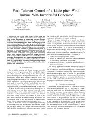
4y [m]121086420−2−4entropy3210−1−2−3−4−5−6−6−4 −3 −2 −1 0 1 2 3 4x [m](a) Trajectories−70 5 10 15 20t [s](b) KF entropiesFig. 1. Simulation results for the KF with modeled detection probability, false alarms and silent periods – true (dashed) and estimated (solid) track states,and tentative but not confirmed tracks (red + marker). The first two objects were detected and a KF was initialized for each one at 0 s. At 5.9 s they wentout the range of the sensors and the entropy of their KF kept rising until they were deleted at 6.3 s. The third object was detected at 3.6 s, and at 9.4 it wentbehind the robot thus causing a rise in entropy. At 11 s it was detected again by the bearing sensor causing an effective drop in entropy. At 15.1 s it movedin front of the robot again and was detected by the location sensor which significantly lowered the entropy.as a sum of the kernels. We continue this approach as proposedin [17], [18], and convert each sample to a kernelK h (ˆx t ) = h n K(ˆx t ), (16)where K(.) is the particle set covariance, and h > ( 0 is the scalingparameter. For the kernel, we choose h =e4n+2)N −e ,where e = 1n+4, and N is the number of particles. At thispoint, each track is described as a sum of Gaussian kernels,p (ˆx t ) = ∑ Ni=1 N (ˆx t(i), 2K h (ˆx t )), for which an analyticalsolution for the quadratic Rényi entropy exists [27]H 2 (x t ) = − log 1 ∑N N∑N 2 N (ˆx t (i) − ˆx t (j); 0, 2K h (ˆx t )).i=1 j=1(17)Due to symmetry, only half of these kernels need to beevaluated in practice.The track management logic is as follows. When the tracksare initialized, they are considered tentative and the initialentropy is stored. When the entropy of a tentative track dropsfor 50% – it is a confirmed track. If and when the entropygets 20% larger than the initial entropy – the track is deleted.This logic reflect the fact that if the entropy is rising, we arebecoming less and less confident that the track is informative.Furthermore, since no entropy should be greater than the onecalculated at the point of the track initialization, we can usethis initialization entropy as an appropriate deletion threshold.V. SIMULATIONSIn order to test the performance of the algorithm, wegenerated three intersecting circular trajectories. The robotwas at (0, 0, 90 ◦ ) m, the first object started at (2, 1) m andfinished at (−0.8, 10) m, the second object started at (−2, 1)m and finished at (0.8, 10) m, while the third object started at(3, 0) m and finished at (−1.6, 2.5) thus making more than onerevolution around the mobile robot (Fig. 1a). Each object wastracked in an alternating manner by the location and bearingsensor, while the maximum range for both was kept at 6 m.The location sensor can only track objects in front of themobile robot, i.e. from 0 to π, and was corrupted with whiteGaussian noise given by N ([x y] T ; 0, 0.03 · I). The bearingsensor, on the other hand, can only measure the bearing angleθ of the object, but in the full range around the mobile robot,i.e. from 0 to ±π, and was also corrupted with white Gaussiannoise given by N (θ; 0, 3 ◦ ).Furthermore, for both sensors each measurement had thedetection probability of P D = 0.9, and the probability of afalse alarm was P F = 0.01. Since the bearing sensor modelsa microphone array, it is logical to assume that the speaker willhave pauses while talking, thus resulting in longer periods ofabsent measurements. This was modeled by placing a randomnumber of pauses of maximum length of 2 seconds at randomtime instances. Although the assumption about the talkingspeaker might not be realistic for every-day scenarios, we findit important to analyze performance of a bearing-only sensorin such a multisensor system.The tracks can only be initialized by the location sensor,but the existing tracks should be kept by the bearing sensorwhen the object moves behind the robot. Since in this casethe entropy is substantially larger, it requires calculation ofbearing-only initialization entropy, in order to efficiently managethe case when the object is behind the robot.In Fig. 1 we show KF simulation results with added detectionprobability, false alarms, and silent speaker periods, fromwhich we can see that there were several false tracks initiatedbut never confirmed. Furthermore, we made 100 Monte Carlo(MC) runs for the Kalman filter – on average there were 11.43initialized, 7.95 tentative tracks, and 3.48 confirmed tracks. Inan ideal situation we would have had three confirmed tracks,but taking the scenario into account we can conclude that the

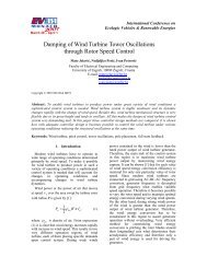
5128106y [m]86420−2entropy420−2−4−4−4 −3 −2 −1 0 1 2 3 4x [m](a) Trajectories−60 5 10 15 20t [s](b) PF entropiesFig. 2. Simulation results for the PF with modeled detection probability, false alarms and silent periods – true (dashed) and estimated (solid) track states,and tentative but not confirmed tracks (red + marker). The objects trajectories were the same as in the case of the KF. The main difference is in the thirdobject’s estimated trajectory: when the object moved behind the robot, there were bearing measurements up to 13.8 seconds when a silent period started. Theentropy kept rising and the object was deleted before new measurements appeared. The object moved in front of the robot at 15.1 and consequently a newfilter was initialized.algorithm performs well when it comes to tracking, associationand track management.The results of the simulation for the PF with added detectionprobability, false alarms, and silent speaker periods are shownin Fig. 2. Furthermore, we also made 100 Monte Carlo (MC)runs for the particle filter – on average there were 8.17initialized, 3.22 tentative, and 4.95 confirmed tracks. Althoughthe average number of confirmed tracks was larger than in thecase of the Kalman filter, we still find it to be of acceptableperformance.Simulations were performed on a machine running at 2.33GHz with an unoptimized Matlab implementation. The averagecomputational time of each iteration was 1.9 ms and137.2 ms for the KF and PF, respectively. Time spent on theentropy calculation was 0.02 ms and 88.6 ms for the KF andPF, respectively.VI. EXPERIMENTSTo further test the proposed approach, we conducted experimentswith our Pioneer 3-DX robot. The laser sensor was theSick LMS 200 model, while the microphone array is of ourdesign. Furthermore, since the proposed framework is easilyextended to multiple sensors, we also used the Kinect time-offlightcamera with a face recognition algorithm based on [28]to yield a set of measurements in 3D. In the experiment twopeople were walking in an intersecting trajectory in front ofthe robot (a snapshot of the experiment is shown in Fig. 3).The results are shown in Fig. 4 from which we can see that thefirst person (blue line) started at (−1.2, 2.3) m and finishedat (0.9, 2.3) m, while the second person (green line) startedat (0.7, 0) m and finished at (0.6, 0) m. The first person wasin the field-of-view (FOV) of all the three sensors and wastalking throughout the experiment, while the second personentered LRS FOV at a later time, kept quiet and was facingthe robot only in the second half of the trajectory. Tracks wereFig. 3. A snapshot of the data acquisition and signal processing for theexperiments. The measurements were classified and collected based on ourprevious work [10], [11], [15], with only the signal processing stage done,i.e. no tracking was performed on the sensor level.correctly initialized and maintained, despite the large numberof false alarms. The second track was deleted short-after thesecond person left the LRS FOV.VII. CONCLUSIONIn the present work we addressed the problem of trackingmultiple objects with multiple heterogeneous sensors – specificallyan LRS, a microphone array, and an RGB-D camera. Theintegration of multiple sensors is solved by asynchronouslyupdating the tracking filters as new data arrives. We solvedthe data association problem by applying the JPDAF, which isa suboptimal zero-scan derivation of the MHT, but which ineffect assumes a known number of objects. To circumvent thisassumption, we proposed an entropy based track management

6524130y [m]2entropy−11−20−3−1−4 −3 −2 −1 0 1 2 3x [m](a) People trajectories−40 5 10 15 20 25 30 35 40t [s](b) KF entropiesFig. 4. Experimental results for the KF – estimated (solid) track states, and tentative but not confirmed tracks (red + marker). The first object was in thescene from the beginning, while the second object entered the scene at 7.5 s. At 15 s the second object got occluded by the first, which caused an increasein entropy, while at 30 s the second object occluded the first shortly before exiting the scene. The false alarms were caused by tiles on the wall and leg-likefeatures in the room (chairs and tables).scheme, and demonstrated its performance for the Kalman andparticle filter both in simulation and experiment. The resultsshowed that the proposed algorithm is capable of maintaininga viable number of filters with correct association and accuratetracking.ACKNOWLEDGMENTThis work was supported by the Ministry of Science,Education and Sports of the Republic of Croatia under grantNo. 036-0363078-3018.REFERENCES[1] A. Almeida, J. Almeida, and R. Araújo. Real-time Tracking ofMultiple Moving Objects Using Particle Filters and Probabilistic DataAssociation. AUTOMATIKA Journal, 46(1-2):39–48, 2005.[2] K.O. Arras, S. Grzonka, M. Luber, and W. Burgard. Efficient peopletracking in laser range data using a multi-hypothesis leg-tracker withadaptive occlusion probabilities. In IEEE ICRA, pages 1710–1715.IEEE, 2008.[3] Y. Bar-Shalom. Extension of the probabilistic data association filterto multi-target environment. In Proceedings of the 5th Symposium onNonlinear Estimation, pages 16–21, San Diego, CA, 1974.[4] N. Bellotto and H. Hu. Vision and Laser Data Fusion for TrackingPeople with a Mobile Robot. In Proceedings of the IEEE InternationalConference on Robotics and Biomimetics, pages 7–12, 2006.[5] S. Blackman and R. Popoli. Design and Analysis of Modern TrackingSystems (Artech House Radar Library). Artech House Publishers, 1999.[6] I.J. Cox. A review of statistical data association techniques for motioncorrespondence. International Journal of CV, 10(1):53–66, 1993.[7] I.J. Cox and S.L. Hingorani. An Efficient Implementation of Reid’sMultiple Hypothesis Tracking Algorithm and its Evaluation for thePurpose of Visual Tracking. Trans. on PAMI, 18(2):138–150, 1996.[8] T. Fortmann, Y. Bar-Shalom, and M. Scheffe. Sonar tracking of multipletargets using joint probabilistic data association. IEEE Journal ofOceanic Engineering, 8(3):173–184, July 1983.[9] D.L. Hall and J. Llinas. An Introduction to Multisensor Data Fusion.Proceedings of the IEEE, 85(1):6–23, 1997.[10] S. Jurić-Kavelj and I. Petrović. Experimental comparison of AdaBoostalgorithms applied on leg detection with different range sensor setups.In 19th International Workshop on RAAD, pages 267–272. IEEE, 2010.[11] S. Jurić-Kavelj, M. Seder, and I. Petrović. Tracking Multiple MovingObjects Using Adaptive Sample-based Joint Probabilistic Data AssociationFilter. In Proceedings of 5th International Conference on CIRAS,pages 99–104, Linz, Austria, 2008.[12] A. Kräußling and D. Schulz. Tracking extended targets—a switchingalgorithm versus the SJPDAF. In Proc. of FUSION, pages 1–8, Florence,Italy, 2006.[13] M. Luber, G.D. Tipaldi, and K.O. Arras. Spatially grounded multihypothesistracking of people. In Workshop on People Detection andTracking, 2009 IEEE ICRA, Kobe, Japan, 2009.[14] R. Luo and M. Kay. Multisensor Integration and Fusion in IntelligentSystems. IEEE Transactions on Systems, Man, and Cybernetics,19(5):901–931, 1989.[15] I. Marković and I. Petrović. Speaker Localization and Tracking witha Microphone Array on a Mobile Robot using von Mises Distributionand Particle Filtering. Robotics and Autonomous Systems, 58(11):1185–1196, November 2010.[16] C Martin, E Schaffernicht, A Scheidig, and H.-M. Gross. Multi-ModalSensor Fusion using a Probabilistic Aggregation Scheme for PeopleDetection and Tracking. Robotics and Autonomous Systems, 54(9):721–728, September 2006.[17] C. Musso, N. Oudjane, and F. Le Gland. Improving Regularised ParticleFilters, pages 247–272. Springer-Verlag, 2001.[18] L.-L.S. Ong. Non-Gaussian Representations for Decentralised BayesianEstimation. PhD thesis, The University of Sydney, 2007.[19] L.Y. Pao and S.D. O’Neil. Multisensor fusion algorithms for tracking.In Proceedings of the ACC, pages 859–863, San Francisco, CA, 1993.[20] E. Parzen. On Estimation of a Probability Density Function and Mode.The Annals of Mathematical Statistics, 33(3):1065–1076, 1962.[21] E. Prassler, J. Scholz, and A. Elfes. Tracking multiple moving objectsfor real-time robot navigation. Autonomous Robots, 8(2):105–116, 2000.[22] D. Reid. An algorithm for tracking multiple targets. IEEE Transactionson Automatic Control, 24(6):843–854, December 1979.[23] A. Rényi. Probability Theory. North-Holland, London, 1970.[24] J. Richardson and K. Marsh. Fusion of Multisensor Data. TheInternational Journal of Robotics Research, 7(6):78–96, 1988.[25] D. Schulz, W. Burgard, D. Fox, and A.B. Cremers. People Tracking withMobile Robots Using Sample-Based Joint Probabilistic Data AssociationFilters. The International JRR, 22(2):99–116, February 2003.[26] M. Seder and I. Petrović. Dynamic window based approach to mobilerobot motion control in the presence of moving obstacles. In Proceedingsof IEEE ICRA, pages 1986–1991, Roma, Italy, 2007.[27] K. Torkkola. Feature Extraction by Non-Parametric Mutual InformationMaximization. Journal of Machine Learning Research, 3(7-8):1415–1438, October 2003.[28] P. Viola and M. Jones. Robust real-time object detection. InternationalJournal of Computer Vision, 2002.[29] G.A. Watson and W.D. Blair. Tracking Maneuvering Targets withMultiple Sensors Using the Interacting Multiple Model Algorithm.Proceedings of SPIE, 1954:438–449, 1993.