facet-based surfaces for 3d mesh generation - CiteSeerX

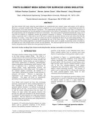
FACET-BASED SURFACESFOR 3D MESH GENERATIONSteven J. Owen 1 , David R. White 2 , Timothy J. Tautges 31,2,3 Sandia National Laboratories*, Albuquerque, NM U.S.A sjowen@sandia.gov2 Carnegie Mellon University, Pittsburgh, PA U.S.A drwhite@sandia.gov3 University of Wisconsin, Madison, WI U.S.A tjtautg@sandia.govABSTRACTA synthesis of various algorithms and techniques used for modeling and evaluating facet-based surfaces for 3D surface meshgeneration algorithms is presented, including implementation details of how these techniques are used within an existing meshgeneration toolkit. An object oriented data representation for facet-based surfaces is described. Numerical techniques fordescribing G 1 continuous curves and surfaces from triangles forming quartic Bézier triangle patches is presented. A combinationof spatial searching and minimization techniques to solve the smooth surface projection problem are described. Examples andperformance of the proposed methods are put in context with relevant surface mesh generation problems.Keywords: facetted models, 3D surface mesh generation, closest point, Walton patch1. INTRODUCTIONComputational simulations of physical processes modeledusing finite element analysis frequently employ complexautomatic mesh generation techniques. Robust geometricrepresentations of the physical domain are generallyrequired in order for mesh generation algorithms to bereliable. Solid models or boundary representation (b-rep)models are most frequently employed, typically providedthrough a commercial computer aided design (CAD)package or third party library.Since automatic mesh generation algorithms must mesh anunderlying solid model, a geometry kernel is frequentlyprovided via an application programmers interface (API).A small set of geometry and topology queries are sufficientto provide automatic mesh generation algorithms withenough information to generate a mesh for computationalsimulation.Since mesh generation algorithms usually access thegeometry representation via an API, any underlyingrepresentation of the geometry may be used, provided itmeets the requirements of the prescribed API. In mostcases the underlying API is a b-rep model where curves andsurfaces are described by analytic expressions or nonuniformsrational b-splines (NURBS). B-rep models basedon NURBS have become commonplace in the computeraided engineering (CAE) community. Popular CADmodeling packages use NURBS as the basis of theirgeometry kernels, frequently integrating automatic meshgeneration algorithms as an added feature.In recent years, facetted models have become moreimportant as an alternative geometry representation fromNURBS representations. Complete 3D geometric modelscan be represented as a simply connected set of triangles.In many cases, facetted models may be preferred or may bethe only representation available. For example, wherenatural processes are simulated such as in bio-medical orgeo-technical applications, NURBS representations can bedifficult or impossible to fit to the prescribed data. Even ifan initial NURBS representation is used to model amachined part, subsequent large deformations computedfrom an FEA analysis may make the NURBS datairrelevant. A facetted model may be the only alternativefor remeshing or refinement on a deformed model.Additionally, facets in the form of STL (stereo lithography)or graphics files, may be a convenient or even last-ditchform of geometry transfer when other representations areunavailable or inadequate. Furthermore, in some cases alegacy FEA mesh may be the only geometric representationavailable of the model. Extracting the surface faces from*Sandia is a multiprogram laboratory operated by Sandia Corporation, a Lockheed Martin Company, for the United States Department of Energyunder Contract DE-AC04-94AL85000

the elements to form facets is one alternative to provide ageometric model for subsequent design studies.In the ideal case, mesh generation software has beendesigned to work through a generic API, not relying on anyspecific geometry representation. When this is the case, afacetted representation may conveniently replace or serveas an alternative geometry kernel with little or no change tothe mesh generation algorithms themselves. The objectiveof the current work is to propose such a system. Significantprior work has gone into developing a mesh generationtoolkit [1], consisting of a wide variety of algorithms[2,3,4,5,6] that will access a generic geometry kernelthrough a common geometry module [7]. Although thecommercial third party library, ACIS [8], has beensuccessfully used as a NURBS-based geometry kernel, analternative facet-based geometry representation isproposed. It does not necessarily replace the ACISrepresentation, but serves to enhance the existing capabilityof the mesh generation toolkit.This work is a synthesis of a variety of algorithms andtechniques used to successfully model surfaces forpurposes of mesh generation. This work does not presentor promote any specific meshing algorithm, but insteadproposes a geometry system that can be utilized by ageneric 3D meshing algorithm.We first present some background to the problem in orderto put the subsequent discussion into perspective. We willthen describe the data representation used followed by adetailed description of the numerical formulation of thesurfaces. Details of how the facetted surface representationis used within the context of 3D surface meshing will thenbe described along with relevant performance data.Finally, several examples will be presented, showingtypical use of the facetted representation for 3D meshgeneration.2. BACKGROUND2.1 Previous WorkSeveral authors have presented similar facet-based systemsfor use with specific mesh generation algorithms. Forexample, Rypl and Bittnar [9] propose a method forevaluating facet-based surfaces based upon interpolationsubdivision. This method utilizes the hierarchal recursiverefinement of the facets. Control points for a triangularBézier patch are positioned by computing a weightedaverage of neighboring nodes resulting in a C 1 surface.Their facet-based surface representation is employed with a3D advancing front triangle meshing algorithm. Frey andGeorge [10] also provide details on the use of triangleBézier patches for modeling surfaces of prescribedcontinuity for application to finite element meshgeneration. Additionally, Frey [11], and Laug andBorouchaki [12] address issues related to parametric spacemesh generation on facet-based surfaces. The currenteffort, in contrast addresses integration of a facet-basedsystem as a geometry kernel for 3D surface meshgeneration.The current work extends the previous work of the authors[13] where a method for decomposing a finite elementmodel to generate a complete geometric model for meshgeneration was proposed. Sets of facets were generatedand grouped together to form surfaces based upon userdefined feature angle criteria and boundary condition data.The current work assumes that facets have been adequatelygrouped into topological surfaces as described in [13].2.2 Surface MeshingSurface meshing algorithms may be characterized as eitherparametric or 3D. A parametric surface-meshing algorithmcreates the mesh in a two-dimensional space, mapping thefinal nodal coordinates to three dimensions only as a finalstep. Many examples of parametric surface meshing existin the literature [14,15,16]. Fundamental to parametricmeshing is a global 2D parametric (u,v) representation forthe entire surface. NURBS representations provided byCAD modelers conveniently provide this information. Forfacetted models, however, surface parameterizations are noteasy to come by and are a topic of active research [17,18].3D meshing algorithms, on the other hand, do not requirean underlying parameterization. Rather than mappingbetween 2D and 3D spaces, the meshing algorithm isperformed completely within the 3D space. The currentwork restricts its application to 3D meshing algorithms,leaving parametric meshing to subsequent research.Paving [2] and 3D advancing front triangle meshing [19]are examples of 3D meshing algorithms. These algorithmsbegin with an outer loop of mesh edges and begin placingelements on the surface marching systematically from theboundary towards the interior. Fundamental to thesealgorithms is the evaluation of the underlying surface. Theclosest point or projection routine combined with surfacenormal evaluations at a point are the main requirementsthese algorithms demand of the geometry kernel. While inmost cases these functions are standard API calls availablefrom a NURBS-based geometry system, they must bedefined for a facet-based system. This work proposesseveral techniques for defining these routines for facetbasedrepresentations.2.4 G 0 SurfacesThe facet representation can be characterized by thegeometric continuity for which the composite set oftriangles comprising a surface will maintain.For purposes of this work, we will not consider parametriccontinuity (ie. C 0 ,C 1 , …), as 3D surface meshing schemeswill be employed. Instead G 0 and G 1 continuousrepresentations will be considered. Farin [20] details therequirements of continuity across surface patchescomposed of Bézier patches. Kashyap [21] addresseshigher order continuity between triangle patches.A surface maintaining G 0 continuity guarantees only thatthat the facet edges meet edge-to-edge, without gaps. Inthis case, characteristic facets and ridges between trianglesmay be evident. In many cases, G 0 is sufficient toadequately characterize the surface for mesh generation.Planar surfaces, surfaces with large curvature or surfaces

with sufficiently dense triangles to represent curvature, maynot require more than what a G 0 facet representation willprovide. Since higher order representations will inevitablybe more expensive, the option to provide for G 0representations should be supplied in a facet-basedgeometry kernel for mesh generation.Triangles may be conveniently parameterized usingBarycentric coordinates. Instead of the standard u,vparameterization of tensor product surfaces, threeparameters, u,v,w, are used, where u+v+w=1 and u,v,w ≥0.Figure 1 shows the characteristic parametric domain forany triangle.triangle patch. For example, Figure 2 shows the polarcoordinate locations for triangle patches n=3 and n=4.Figure 2. Polar values for triangles patches of n=3and n=4It has been established that the minimum order of a triangleBézier patch necessary to model a G 1 surface is n=4 [22].For this case, equation (3) can be written as:Figure 1. Barycentric coordinate system definedon a triangle.Using Barycentric coordinates (u,v,w) any point X in thedomain may be defined as:X( uvw , , ) = uP + vP + wP (1)0 1 2where P 0 , P 1 , P 2 are the vertices of the triangle. In a similarmanner, the normal at point X can be approximated as:NX ( uvw , , ) = uN0 + vN1+wN 2(2)where N 0 , N 1 , N 2 are the approximated normals at pointsP 0 , P 1 , P 2 respectively.2.2 G 1 SurfacesIt may be necessary to provide a smooth approximation tothe surface. To do so, Bézier triangular patches may bedefined. A degree n triangular Bézier patch may bedescribed with the following equation:X( uvw , , ) = ∑ B ni, j, k( uvw , , ) Pi, j,k(3)Bi+ j+ k=nn!= u v w(4)i! j! k!n i j ki, j,kP i,j,k are the control points of the triangle and B i,j,k (u,v,w)can be thought of as the weights at polar location i,j,k,where i+j+k =n. Note also that equation (1) can bethought of as a special case of equation (3) where n=1. Inthis case B ijk =1 for all i,j,k.Triangular polar values are a convenient way ofgeneralizing the control point indices for an arbitrary( , , )4X uvw = P0,0,4w+3 34P1,0,3uw+ 4P0,1,3vw+2 2 3 2 26P2,0,2uw + 12P1,1,2 uvw + 6P0,2,2vw+3 2 2 3P3,0,1u w+ P2,1,1u vw+ P1,2,1uv w+ P0,3,1v w+4 3 2 2 3 44,0,0u + 43,1,0uv+ 62,2,0uv + 41,3,0uv+0,4,0v4 12 12 4P P P P PWalton [23] describes a procedure for defining P i,j,k as afunction of the triangle vertex locations P i {i=0..3} andnormals N i {i=0..3}. The Walton patch is central to thetechniques proposed in the present work. How it is usedwithin the context of a practical geometry kernel for meshgeneration is the additional contribution proposed by thecurrent research and development effort. Definition andimplementation of the Walton patch is outlined in section 5.Similarly, smooth normals for the quartic patch at X(u,v,w)may be computed by evaluating a cubic Bézier patch.3N ( uvw x, , ) = N w 0,0,3+2 23N1,0,2uw+ 3N0,1,2vw+2 23N2,0,1uw+ 6N1,1,1uvw+ 3N0,2,1vw+3 2 2 33,0,0u + 32,1,0u v+ 31,2,0uv +0,3,0vN N N NAssuming the normals at N 3,0,0 , N 0,3,0 ,andN 0,0,3 are thecomputed normals at the triangle vertices N 0 , N 1 and N 2respectively, a procedure for computing the remaining N i,j,kby extending the work of Walton is introduced in section 5.3. DATA REPRESENTATIONAs stated in the Introduction, facet-based surfaceconstruction is employed in a variety of contexts. Thesetypes of surfaces can be used to support mesh generation onfacet-based models. The method used to store and evaluatethe facet data can vary according to the source of thosedata. For example, in the context of large-deformationFEA, it is important to maintain links between the originalmesh and the corresponding facets used to model thesurface. Also, for these analyses, duplication and updatingof facet data can be problematic because of memorylimitations commonly found in parallel computing(5)(6)

environments and because position and topology of facetsmay be changing. Facets originating from STL or graphicsfiles may not have those limitations. In contrast, thefunctions needed to support mesh generation do not dependon the source of the facets being evaluated, and thereforeshould look the same regardless of the facet representation.We accomplish both these goals utilizing inherited classesin C++ for our facet data structure.We define a generic FacetEntity class, from which genericPoint, FacetEdge and Facet classes are derived. Containedin these classes is the normal and control point datanecessary to describe the G 1 surface approximation. Asimplified representation of the data contained in theseclasses is illustrated in Figure 3.class FacetEntity {}class Facet : public FacetEntity {Vector3D *controlPoints;Vector3D normal;Box boundingBox;virtual get_points() = 0;}class FacetEdge : public FacetEntity {Vector3D *controlPoints;Boolean isFeature;virtual get_adjacent_facets() = 0;}class Point : public FacetEntity {List normalList;virtual get_location() = 0;virtual get_adjacent_facets() = 0;}class PointNormal (Vector3D normal;int surfaceID;}Figure 3. Simplified C++ classes used for definingfacet representationThese classes also support typical functionality like pointlocation and point-edge-facet adjacency. These functionsare defined as virtual functions to allow representationspecificversions to be implemented. An exampleinheritance tree for the facet representation is illustrated inFigure 4.The actual implementation of the functions described aboveis done in classes derived from Facet, FacetEdge and Point.We describe here two specific implementations: one thatstores the facet data in the actual derived classes, and onethat references those data from an analysis application. Inthe first child class, PointData, the point data (i.e.coordinates and adjacency information) are stored in theclass and are used directly to implement the requiredfunctions. This is illustrated in Figure 4 in the box markedA. The second implementation example, in the FEAPointclass, does not store the point data in the class; those dataare retrieved from the mesh objects in the FEA code, towhich the FEAPoint object keeps a pointer. Box B inFigure 4 illustrates this case. Implementations of theFacetEdge and Facet classes are similar to those for Point.Figure 4. Inheritance tree for object oriented facetrepresentationThe proposed object oriented implementation also leavesopen the possibility for additional code reuse. Otherapplications need only supply the required topologyinformation for the facets in order to take advantage of theproposed surface representation and evaluation.4. FACET INITIALIZATION AND EVALUATIONThe following procedure outlines the proposed process forinitializing facet-based surfaces for use as a geometrykernel for 3D mesh generation. Figure 3 illustrates thebasic data needed to sufficiently describe the smoothsurface. Control point and normal data necessary tocompute equations (5) and (6) are necessary. Dependingon the speed vs memory requirements of the application,this data may be precomputed and stored with the facetentities or may be computed only as evaluations arerequired. For the mesh generation applications used withthis work, it was found that pre-computing the normal andcontrol point data was more efficient.It should be noted that curves and surfaces with zerocurvature can be accurately modeled with a G 0 surfacerepresentation. Given that many surfaces used to modelmachined parts have flat surfaces, it is worthwhile to checkfor this condition and only initialize those with anycurvature. Furthermore, it may be worthwhile to perform aninitial decimation of the facets comprising the surface toreduce memory requirements and increase the performanceof the closest_point operation discussed later.The initialization procedure begins first with theapproximation of the normals at the Points. The normalsare then used as input to compute the control points on theFacetEdges. Finally, the control point data on the Facets iscomputed using the FacetEdge control points. Details forinitializing each of these data objects is now described.4.1 PointsThe definition of Bézier triangle facets requires normals tobe provided or approximated at each of the facet vertices.If normals are available from an external source, such asthose provided through an STL format, these should ideally

e used. If they are not provided, it is necessary toapproximate them. Reference [13] describes the methodused in the current work, defining the normal, N P at a pointas the weighted average of the adjacent facets, N j ,wherethe weight, w j is the normalized facet angle at the point.Equations (7), (8) and Figure 5 describe this procedure.nN = ∑N w(7)P j jj = 1αiw i = n∑αii=1(8)Figure 6. FacetEdge required input to computecontrol points P i,jN 6N 5PN Pα 1α 2α 3N 4N 1N 2N 3Figure 5. Definition of a normal at point PAt feature breaks, it is necessary to compute multiplenormals at a point, where the normal is the weightedaverage of only the facet normals defined on a givensurface. Figure 3 describes the Point class as containing alist of PointNormal objects. The PointNormal objectcontains both the computed normal and a reference to thesurface to which it applies. It should be emphasized thatthis extra information is only required at breaks or surfaceboundaries to distinguish surface features and is onlyallocated at the Points as needed to ensure minimaladditional memory overhead.4.2 Facet EdgesTo completely represent the quartic Bézier facet edge, fivecontrol points are needed. In addition to serving as thecontrol points for the boundary curves, The control pointson the FacetEdges are utilized in the definition of thetriangle Bézier patches (discussed later) that areimmediately adjacent the FacetEdge. Adjacencyinformation provided by the data representation describedin the previous section is necessary to keep track of thisdata and utilize it as necessary.Since we may utilize the Point locations for the ends of theBézier curve, the remaining three control points, P i, j{j=1..3} may be stored with the FacetEdge. In practice, therequired input to compute P i,j (Figure 6) are the FacetEdgeendpoints P i , P i+1 , the surface normals, N i , N i+1 and thecurve tangent vectors, T i , T i+1 at the same points.It is assumed that point P i and P i+1 are provided. Theprevious section addresses approximation of normals N i ,N i+1 . In order to maintain G 0 continuity between adjacentfacet-based surfaces, it is necessary to approximate thecurve tangents, T i , T i+1 . For edges on the interior of thesurface where G 1 continuity is to be maintained, it issufficient to define both T i and T i+1 as the direction of theFacetEdgePTi= Ti+1=Pi+1i+1− Pi− PFor edges marked as Features, using equation (9) mayresult in gaps between the facets as illustrated in Figure 7.In this example a cylinder has been represented with acoarse set of facets. Facet A and Facet B are on differentsurfaces, but are required to meet at edge P i P i+1 . Usingonly the facet normals and the tangents of equation (9),gaps between the facets would result in different P i,j for thesame edge depending upon which facet is used for thecomputation. This is illustrated in Figure 7 by (P i,j ) A and(P i,j ) B computed from Facet A and Facet B respectively.Instead, the following logic is employed:⎧L 11 cos( ),i Lii i θ−⎪L⋅ L −

1 1i,2 = i,1 + i,22 2P V V (24)3 1i,3 = i,2 + i+ 14 4P V P (25)In the current work, P i,j from equations (23) to (25) arestored with the FacetEdge. To further ensure continuitybetween facets on adjoining surfaces, it is necessary toaverage the final locations P i,j computed with respect toeach adjoining facet.Sincetheobjectiveofthisexerciseistoprovideameanstoevaluate equation (5), the following correspondence existsbetween the points P i,j,k defined with polar indices, P i andP i,j .Figure 7. Cylinder represented by coarse facets.Tangent vectors required to maintain G 0continuity between surfaces.Figure 7 illustrates the location of point (P i ) prev and(P i+1 ) next . These are the previous and next vertices onadjacent FacetEdges to P i and P i+1 respectively that are on afeature edge. Note that multiple feature edges may meet ata single point P. In this case, the appropriate selection of(P i ) prev and (P i+1 ) next must be determined from localtopology by traversing FacetEdges in order at P i and P i+1 tolocate the next FacetEdge marked as a feature.Armed with the six vectors described in Figure 6, we arenow prepared to compute the three control points P i,j{j=0..3}. The procedure used is defined in Walton andMeeks [23], but is illustrated here for clarity. Note themodification to the Walton patch to accommodate thetangent vectors defined in equations (10) and (11) at featureedges.d i = i+1 − iP P (15)N N (16)a i = i ⋅ i+1a = N ⋅T (17)i,0i ia i,1 = i+ 1 ⋅ i+1N T (18)6(2 a + aa )ρ =ii,0 i i,124 − ai6(2 a + aa )σ =ii,1= i +i,1 i i,024 − aii(6Ti − 2 Ni + Ni1)18(19)(20)d ρ σV P +(21)d ρ σV P (22)i,2 = i+1 −i(6Ti+ 1+ Ni + 2 Ni+1)181 3i,1 = i + i,14 4P P V (23)P = P P = P P = P P = PP = P P = P P = P P = PP P P P P P P P4,0,0 0 0,3,1 0,1 1,0,3 1,1 3,1,0 2,10,4,0 1 0,2,2 0,2 2,0,2 1,2 2,2,0 2,20,0,4 = 2 0,1,3 = 0,3 3,0,1 = 1,3 1,3,0 = 2,34.3 Facets(26)Making use of the control points on the FacetEdges, thequartic Bézier patch, control points P 1,1,2 , P 2,1,1 and P 1,2,1 onthe interior of the facet can now be defined. The locationsof these points are critical to describing G 1 continuitybetween adjoining patches. Walton and Meeks propose amethod, whereby two candidate locations for interiorcontrol points are defined for each FacetEdge, resulting insix vectors G i,j {i=0,1,2; j=0,1}. Final locations for interiorcontrol points P 1,1,2 , P 2,1,1 and P 1,2,1 are a function of theevaluated (u,v,w) parameters and G i,j . Once again theprocedure outlined by Walton and Meeks is described herefor clarity.For each FacetEdge, i, in the Facet, compute the following:W = V −P (27)i,0 i,1W = V −V (28)i,1 i,2 i,1W = P −V (29)i,2 i+1 i,21Di,0 = Pi,3 − ( Pi,1+ P i )(30)21Di,1 = Pi,1− ( Pi+1 + P i,3)(31)2i×i,0Ai,0= N WWi,0i+ 1 i,2Ai,2= N × WWi,2Ai,1=Ai,0 + Ai,2Ai,0 + Ai,2(32)(33)(34)

λi,0λi,1D=WD=W⋅ W⋅ Wi,0 i,0i,0 i,0⋅ W⋅ Wi,1 i,2i,2 i,2i,0 i,0 i,0(35)(36)µ = D ⋅A (37)µ = D ⋅A (38)i,1 i,1 i,2The two control points G i,0 , G i,1 with respect to FacetEdge imay now be defined as:1Gi,0 = ( Pi,1 + Pi,2)22 1+ λi,0 Wi,1 + λi,1 Wi,03 32 1+ µ i,0 Ai,1 + µ i,1 Ai,03 31Gi,1 = ( Pi,2 + Pi,3)21 2+ λi,0 Wi,2 + λi,1 Wi,13 31 2+ µ i,0 Ai,2 + µ i,1 Ai,13 3(39)(40)In practice, the six control points, G i,j are stored with theFacet object. When the facet is to be evaluated, interiorcontrol points P 1,1,2 , P 2,1,1 and P 1,2,1 may be uniquelyevaluated as:only as needed. If they are precomputed, Two additionalcontrol points per FacetEdge, N i,0 and N i,1 would becomputed and stored. In this case we may take advantageof the cross edge derivative information computed inequations (30) and (31).Ni,0=Ni,1=Di,0 × Wi,0Di,0 × Wi,0Di,1 × Wi,2Di,1 × Wi,2(44)(45)The correspondence between the control points N i,j,k inequation (6) and the N i,j at the FacetEdges defined inequations (44) and (45) is as follows:N3,0,0 = N0 N0,2,1 = N0,0 N1,0,2 = N1,0 N2,1,0 = N2,0N0,3,0 = N1 N0,1,2 = N0,1 N2,0,1 = N1,1 N1,2,0 = N2,1(46)N = N0,0,3 2Remaining to be computed is the internal control point ofthe cubic Bézier. This may be computed when the facet isevaluated using the interior control points from the quarticBézier as follows:N1,1,1=( P1,2,1 − P2,1,1 ) × ( P1,1,2 −P2,1,1)( P1,2,1 − P2,1,1 ) × ( P1,1,2 −P2,1,1)(47)1,1,2 = 1 ( u 2,2 v 0,1 )u+v+P G G (41)1,2,1 = 1( w 0,2 u 1,1)w+u+P G G (42)2,1,1 = 1( v 1,2 w 2,1)v+w+P G G (43)Finally, in order to evaluate the Bézier facet at parameter(u,v,w), equation (5) may be employed by using the controlpoints defined in equation (26) and equations (41) to (43).Care must be taken to extract the appropriate control pointsin the correct order from the FacetEdges and Points so thatcontrol points P i,j,k are appropriately assigned.4.4 NormalsSurface normals may be computed by evaluating the cubicBézier of equation (6). Once again the normals computedat the facet vertices N 0 , N 1 , N 2 can be used for the controlpoints N 3,0,0 , N 0,3,0 and N 0,0,3 respectively. Left to becomputed are the seven remaining control points: two peredge and one at the center of the triangle.As with the calculation of the quartic control points,depending upon the speed vs. memory requirements of theapplication, the normals for the cubic patch of equation (6)may be precomputed and stored, or they may be computedFigure 8. Quartic control point grid showingrelationship to cubic grid of normals.In practice, rather than storing N i,j for each FacetEdge, N i,jmay be computed only as needed. Instead of regeneratingthe cross derivatives D i,j for equations (44) and (45), thenormals N i,j can be derived directly from the control pointsof the quartic Bézier in a similar manner to equation (47).Figure 8 shows the relationship between the quartic controlpoint grid and the normals required for the cubic Bézierpatch. The normal of a local triangle in the quartic Béziercontrol grid should provide a sufficient approximation tothe cubic Bézier control points. Therefore, the controlpoints for the cubic Bézier can be determined as follows:

Ni, j,k=( Pi, j+ 1, k− Pi+ 1, j, k) × ( Pi, j+ 1, k−Pi+1, j,k)( i, j+ 1, k− i+ 1, j, k) × ( i, j+ 1, k−i+1, j,k)P P P P (48){ i+ j+ k = 3, } { i, j, k ≥0}4.5 FacetEdge Evaluation3D mesh generation algorithms frequently require thecurves to be evaluated. Since we have defined our curvesto be a set of FacetEdges, curve evaluation can utilize thecontrol point information stored with the FacetEdge. Oneapproach is to utilize equation (5), setting one of theparameters (u,v,w) to zero. This method however requirescomputing unnecessary control point information on thefacet. Instead, the standard Bézier equation may be used:nnP() t = ∑ Bi() t Pi(49)i=0n n!n−iBi() t = 1−t ti! n i !( ) ( ) −i(50)For the quartic case, evaluation of the FacetEdge, i, Béziercurve at parameter t { 0≤t≤1}using the facet vertices P 0 ,P 1 and edge control points P i,j (equations (23) to (25)) maybe defined as:X( t) = P(1 − t) + 4 P (1 − t)t +6 P (1 ) 4 P (1 ) P4 3ii,12 2 3 4i,2 − t t +i,3 − t t +i+1t(51)The tangent vector along the edge may also be computedby evaluating a cubic Bézier.T( t) = T(1 − t) + 3 T (1 − t) t + 3 T (1 − t)t + T t (52)3 2 2 3i i,1 i,2 i+1where T i and T i+1 are defined by equations (9) to (11) ormore generally T i,j may be defined as:{ }Ti, j= Pi, j+1− Pi, jj = 0...3(53)5. CLOSEST POINTThe most common API request for 3D mesh generationalgorithms is the closest point, or surface projection: givenan arbitrary point in space, X, find the closest point on thesurface X s . Since this procedure may be called thousandsof times to mesh a single surface, an efficient method issought to perform this operation.The closest point calculation involves two main steps. Thefirst task is selection of a small list of facets close to Xfrom which to evaluate. Once this is determined aminimization procedure is employed for finding the closestpoint on the facet and the distance from X to each facet inthe list is computed. The facet whose computed distance issmallest is selected as X s .5.1 Closest FacetAn obvious solution to the closest facet problem is toproject point X to each of the facets in the surface andselect the point that is the least distance from X. Since thiswould be very inefficient, the objective of the closest facetprocedure is to minimize the number of facets that musteventually be evaluated. Various spatial searchingtechniques are available in the literature [24]. Theproposed method involves a combination of two methods.5.1.1 Bounding Box Elimination MethodThe first method is a simple bounding box eliminationmethod. In this case, the axis-aligned bounding box ofeach facet, B f is evaluated and stored with the Facet object(see Figure 3). This may be done once for each facet uponinitialization of the facet surface. Care should be taken toutilize the Bézier control points in the bounding boxcalculation. Upon projection of point X, a trial axis-alignedbounding box, B X is defined around X such that (B X ) min =X-δ and (B X ) max = X+δ. δ is a small scalar distancerepresentative of the model size. In practice, the diagonalof the model bounding box scaled by 10 -3 is used as theinitial value of δ.Facets selected to evaluate are only those where thebounding box B f overlaps with B X . For this method, everyfacet on the surface must be checked and their boundingboxes verified for overlap. If after checking every facet, nobounding box B f is found to overlap with B X , δ is scaled by2, B X is recomputed and the facets checked again. Thisprocedure continues, scaling δ each time, until at least oneB f is found to overlap with B X . For 3D mesh generationalgorithms, the point to be projected is generally close tothe surface. As a result, in most cases, not more than asingle pass through the facets is required. Care should betaken in choosing an initial δ, as choosing δ too small couldresult in multiple iterations through the facet list beforeencountering any overlap. Choosing δ toolarge,ontheother hand, may result in too many facets being selected toevaluate. This procedure can become expensive as thenumber of facets increase. For this reason an alternatespatial search algorithm is utilized.5.1.2 R-Tree Spatial SearchThe dynamic index structure, R-Tree [25],isusedtofindonly the closest facets to evaluate. The R-Tree structurewas selected because of the multi-dimensional searchstructure of the algorithm. Most spatial search algorithmssuch as octrees and kd-trees [26], are typically only usefulfor storing and retrieving k dimensional data. For instance,problems, which involve finding the closest 3D point, canbe readily solved by octrees. Facet data, however, iftransformed into a single point would require ninedimensional octrees (3 dimensions for each x-y-z locationof each point). Additionally, determining intersections innine dimensional spaces are often error prone. The R-Treedefined by Guttman is specifically designed to handlemutli-dimensional search spaces efficiently. It is a heightbalancedtree with its leaf nodes containing pointers toFacet objects. The structure is designed so that only asmall number of leaf nodes are visited for any searchoperation, however the worst case of the algorithm is notguaranteed to be faster than the traditional n 2 algorithm.The balancing algorithm of the tree is such that this

extreme case will be rare, and in practice the tree appears torun at about O(n) where n is the number of facets.Although relatively efficient, in practice, the overhead ofgenerating and utilizing the additional infrastructure of theR-Tree is not worthwhile for small numbers of facets.Timed tests indicated that using only the bounding boxelimination method was more efficient for up toapproximately 2000 facets. Where additional facets wereneeded to represent a surface, R-Tree was able to improveperformance considerably. As a result, for the currentwork, R-Tree is used only when the number of facets on asurface exceeds 2000.5.2 Closest Point on a FacetLocating the closest point on a facet, F i can be performedon the (hopefully) small list of facets determined fromeither the bounding box elimination method or R-Treesearch. For G 0 surfaces, this is relatively straightforward,as illustrated by the following procedure5.2.1 Projection to a Linear Facet1. Determine the closest point, X p to the planedefined by F i .d = N ⋅X−N ⋅P (54)pFFF0X = X−dN (55)where N F is the facet normal and P 0 is a vertex onF i .2. Determine if X p is inside F i by computing itsbarycentric coordinates with respect to F i .u =v =w =( P2 − P1) × ( Xp−P1)( P − P ) × ( P −P)1 0 2 0( P0 − P2) × ( Xp−P2)( P − P ) × ( P −P)1 0 2 0( P1− P0) × ( Xp−P0)( P − P ) × ( P −P)1 0 2 03. If all parameters u,v,w >0,thenX s = X p(56)(57)(58)4. Otherwise X p is outside F i . Find the closest pointto one of the facet edges or facet vertices.Let P i {i=0,1,2} be the vertex locations on F i ,then project X p to the closest edge based on thefollowing:⎧u< 0, 1⎪i = ⎨v

Given this information, the procedure progresses asfollows:1. First check if X is within tolerance, tol of one ofthe facet vertices. Define a convergence tolerancerelative to the size of facet F i . For example−3tol ≈ area(F ) × 10IF (iX− P < tol) THEN X = P , RETURN.i s i2. Check if A guess is outside the parametric domainof the patch and move it to the parametricboundary.Let A = A guessFOR i=1,2,3; j=(i+1)%3; k=(i+2)%3⎧ A[] i = 0⎪ A[ j]IF ( A[ i]< 0)THEN ⎨A[ j]=(66)⎪ A[ j] + A[ k]⎪⎩A[ k] = 1 −A[ j]3. Let X A =Φ ( A)be the evaluation of the Bézierpatch at parametric location, A (see equation (5))X A =Φ( A )(67)Vmove = X− XA,dmove = V move (68)4. Keep track of the best area coordinate, (A best )thelocation at A best ,(X best ) and its distance from X,(d best ). Initialize with the values computed in (67)and (68). Also keep track of the number ofiterations niter.Abest = A, Xbest = X A,dbest = dmove(69)niter = 0(70)5. Begin Iteration Loop. Check for convergenceand ensure the maximum number of iterations,IMAX has not been exceeded.IF (d move < tol OR niter >IMAX)THENX = X , A = As best S bestRETURN6. Parameters u,v,w are not linearly independent(u+v+w=1). Choose a system, of two variables tooptimize.FOR i=0,1,2; j=(i+1)%3; k=(i+2)%3IF (A[i]>A[j] ANDA[i]>A[k]) THENη = j, ξ = k,ψ = i(71)7. Define area coordinates, AηandAξperturbed asmall distance δ from A. in directionsη andξ respectively.Aη[ η] = A[ η]+ δ⎛ A[ ξ ] ⎞Aη[ ξ] = (1 −Aη[ η]) ⎜1−⎟⎝ A[ ξ] + A[ ψ]⎠Aη[ ψ] = 1 −Aη[ η] −Aη[ ξ]Aξ[ ξ] = A[ ξ]+ δ⎛ A[ η]⎞Aξ[ η] = (1 −Aξ[ ξ]) ⎜1−⎟⎝ A[ η] + A[ ψ]⎠Aξ[ ψ] = 1 −Aξ[ η] −Aξ[ ξ]8. Evaluate at Aηandderivative vectorsη and ξ .Aξand approximateVηandVξin directions(72)(73)Φ( Aη) −XAV η =(74)δΦ( Aξ) −XAV ξ =(75)δ9. Compute a search direction tangent to the BezierpatchNηξ = Vη × V ξ(76)Vmove= ( Nηξ× Vmove)× N ηξ (77)10. Project to 2D coordinate plane based onmagnitude of NηξFOR i=1,2,3; j=(i+1)%3; k=(i+2)%3IF ( Nηξ[ i] > Nηξ[ j]ANDI=j, J=kNηξ[ i] > N ηξ[ k])THENSolve 2× 2 linear equation in I, J system to determine themove distance dη , dξ in the parameter space.Vmove[I] Vξ[I] Vη[I] Vmove[I]Vmove[J] Vξ[J] Vη[J] Vmove[J]dη= , d[I] [I] ξ =Vη Vξ Vη[I] Vξ[I]Vη[I] Vξ[J] Vη[I] Vξ[J]11. Compute the new trial area coordinate A(78)A[ η] = A [ η] + d η(79)A[ ξ] = A [ ξ] + d ξ(80)A[ ψ ] = 1 −A[ η] −A [ ξ ](81)12. Make sure A remains inside the patch. Useequation (66)13. Evaluate X A at A and set up for next iteration.Keep track of the best evaluated location so far.

X = X (82)lastAX =Φ( A )(83)AV = X − X , d = V (84)move A last move moved = X−X (85)XAIF (d X

are computed (Figure 13(a)). Note that multiple normalsmaybecomputedatasinglevertex..(a)(b)Figure 13. (a) Coarse faceting of a cylinder. (b)Computed normals at facet vertices.Once normals are computed, the control points arecomputed on each FacetEdge and Facet. Figure 14 (a)shows the control point grids for each of the facets. Thenormal information can also be computed at this time asshow in Figure 14 (b). Otherwise, the normals may becomputed only as needed.algorithm. Each of these mesh generation algorithmsutilize the facetted surface described in this work.It should be noted that the resulting node locations on thecylindrical surface described by the facetted surfacerepresentation are within tolerance of reproducing theshape of an exact cylinder.The next example (Figure 16) is a contrived modelintended to illustrate the use of the facet-based surfacerepresentation within an H-adaptive environment. In thiscase, facets representing two concentric spheres aredefined. The initial mesh is defined by only quadrilateralelements, which have been split to form facets. The FEAanalysis drives the adaptivity so that the quadrilateralelements are uniformly refined. In this example 3 iterationswere performed resulting in 64 quadrilaterals for everyinitial quad on the surface. New nodes were projected tothe surface defined by the Bézier facetted-surfacerepresentation. The result shown in Figure 16 (b), showsthe resulting refined surface mesh. Once again, theresulting node locations of the refined model generatedonly from the smooth facet representation are withintolerance of an exact sphere.(a)(b)Figure 14. (a) Bezier control point grid from Figure13. (b) Computed normals at the control pointsFigure 15. Facetted model meshed using paving,mapping and sweeping mesh generationalgorithmsHaving set up the facetted surface representation, the modelis ready to be meshed. Figure 15 shows an example meshgenerated on the geometry. In this case, the paving [2]algorithm is used to mesh the cylinder caps and the submappingalgorithm is used to mesh the sides. The interiorhexahedral mesh is generated using the sweeping(a)(b)Figure 16. (a) Coarse faceting of concentricspheres (b) FEA mesh after 3 iterations of H-AdaptivityFigure 17. shows an example of the use of the proposedfacet-based surface representation to improve the resolutionof small features within an existing FEA model. Figure 17(a) shows the initial facetted representation of the model.In this case, the model has small features that are notsufficiently resolved for purposes of the required analysis.After setting appropriate mesh sizing constraints on themodel, the surfaces are remeshed using the pavingalgorithm with results shown in Figure 17 (b). Note theimproved resolution of the interface curves betweenadjoining surfaces. The bold lines illustrate the differencebetween the initial linear representation and the final Bézierrepresentation of the curves.One final example (Figure 18) illustrates the use of thefacet-based surface representation to convert a modelmeshed with triangles into a different element type or tomodify its resolution by remeshing. In some cases, whenonly the FEA mesh is available, to perform design studies,it may be required to change the element type or meshresolution. This can be troublesome when there is nounderlying geometry representation. In this example, thetriangle surface mesh Figure 18 (a) is used as input to the

facet-based surface representation and Bézier patches aregenerated. The paving algorithm is once again used to meshover the original triangle surface mesh. Figure 18 (b) andFigure 18 (c) show the triangle surface mesh remeshed withdifferent resolutions of a quadrilateral mesh. In (b) themesh is coarser than the original mesh and (c), the mesh isfiner.(a)(a)(b)(b)Figure 17. (a) Facet-based model. Enlargedsection shows small features insufficientlyrepresented by the facets. (b) Paving algorithmapplied to the facet-based surface improvesresolution.7. CONCLUSIONFacet-based surface representations have become animportant tool for simulation. Existing mesh generationtools can utilize facet-based surfaces in a similar manner toNURBS-based surfaces through a common API. We haveproposed a variety of technologies necessary tosuccessfully implement curve and surface representationsspecifically for use within an existing mesh generationtoolkit.(c)Figure 18. (a) Initial triangle mesh. (b) remeshedusing Paving. (c) at finer resolutionAn object oriented facet representation has been proposedthat permits flexibility and reuse within differentapplications. Both G 0 and G 1 facet representations havebeen presented, allowing the user to trade off betweenaccuracy and efficiency of the resulting mesh. The Waltonpatch was proposed as the basis for the G 1 facet

epresentation, and its implementation within the context ofa geometry kernel for 3D mesh generation was presented.Additionally, techniques for evaluation of the facetrepresentation during the mesh process were described. Itwas found that in cases with small numbers of facets, thatthe NURBS-based and facet-based representations wereequivalent. However, for significant numbers of facets, theperformance of the facet-based representation was lessefficient. A spatial searching technique, R-Tree, was usedto improve performance for significant numbers of facets.The proposed research has been implemented within thecontext of the Cubit mesh generation software toolkit [1]and is currently utilized by a wide variety of users at the U.S. National Laboratories.REFERENCES[1] CUBIT Mesh Generation Tool Suite: AutomaticUnstructured Hex, Tet Quad and Tri Meshing andSolid Model Geometry Preparation. Web Site:http://endo.sandia.gov/cubit (2002)[2] Blacker, Ted D., "Paving: A New Approach ToAutomated Quadrilateral Mesh Generation",International Journal For Numerical Methods inEngineering, No. 32, pp.811-847, (1991)[3] Roger J Cass, Steven E. Benzley, Ray J. Meyers andTed D. Blacker. “Generalized 3-D Paving: AnAutomated Quadrilateral Surface Mesh GenerationAlgorithm”, International Journal for NumericalMethods in Engineering, No. 39, 1475-1489 (1996)[4] Knupp, Patrick M., "Next-Generation Sweep Tool: AMethod For Generating All-Hex Meshes On Two-And-One-Half Dimensional Geometries",Proceedings, 7th International Meshing Roundtable,pp.505-513, October 1998[5] White, David R. and Timothy J. Tautges, "Automaticscheme selection for toolkit hex meshing",International Journal for Numerical Methods inEngineering, Vol 49, No. 1, pp.127-144, (2000)[6] Borden, Michael, Steven Benzley, Scott A. Mitchell,David R. White and Ray Meyers, "The Cleave andFill Tool: An All-Hexahedral Refinement Algorithmfor Swept Meshes", Proceedings, 9th InternationalMeshing Roundtable, pp.69-76, October 2000[7] "The Common Geometry Module (CGM): AGeneric, Extensible Geometry Interface",Proceedings, 9th International Meshing Roundtable,Sandia National Laboratories, pp.337-348, October2000[8] 3D ACIS Modeler, Spatial Technologies, Web Site:http://www.spatial.com/products/3D/modeling/ACIS.html, (2002)[9] DanielRyplandZdenĕk Bittnar, “Discretizatoion of3D Surfaces Reconstructed by InterpolationSubdivision,” 7 th Conference on Numerical GridGeneration in Computational Field Simulations,pp.679-688 (2000)[10] Pascal J. Frey and Paul-Louis George, “MeshGeneration: Application to Finite Elements,” HermesScience Publishing, Chapter 13.4, pp. 445-448(2000)[11] Pascal J. Frey, “About Surface Remeshing”,Proceedings, 9 th International Meshing Roundtable,pp. 123-126 (2000)[12] P. Laug and H. Borouchaki, “Adaptive ParametricSurface Meshing Based on Discrete Derivatives,” 7 thConference on Numerical Grid Generation inComputational Field Simulations, pp. 719-728(2000)[13] Steven J. Owen and David R. White, “Mesh-basedgeometry: A systematic approach to constructinggeometry from a finite element mesh”, Proceedings,10 th International Meshing Roundtable, pp. 83-96(2001)[14] Tristano, Joseph R., Steven J. Owen, and Scott A.Canann, "Advancing Front Surface Mesh Generationin Parametric Space Using a Riemannian SurfaceDefinition", 7th International Meshing Roundtable,pp.429-445, October 1998[15] George P. L., and H. Borouchaki, DelaunayTriangulation and Meshing Application to FiniteElements, Editions HERMES, Paris, 1998[16] Cuilière, J. C., An adaptive method for the automatictriangulation of 3D parametric surfaces, ComputerAided Design, Vol 30(2), pp.139-149, 1998[17] Sheffer, Alla and E. de Struler, "SurfaceParameterization For Meshing by TriangulationFlattening", Proceedings, 9th International MeshingRoundtable, pp.161-172, October 2000[18] Michael S. Floater, “Parametrization and SmoothApproximation of Surface Triangulations,”Computer Aided Geometric Design, Vol 14, pp.231-250, 1997[19] Lau, T.S. and S.H. Lo, "Finite Element MeshGeneration Over Analytical Surfaces", Computersand Structures, Elsevier Science Ltd, Vol 59, No. 2,pp.301-309, 1996[20] Gerald Farin, “Curves and Surfaces for CAGD”, 5 thEd. Academic Press (2001)[21] Praveen Kashyap, “Geomeric interpretation ofcontinuity over triangular domains,” Computer AidedGeometric Design No. 15 pp. 773-786 (1998)[22] B. Piper, “Visually Smooth Interpolation withTriangular Bezier Patches”, in Farin, G. (Ed.)Geometric Modeling: Algorithms and New TrendsSIAM Philadelphia (1987) pp 221-233[23] D. J. Walton and D.S. Meek, “A triangular G 1 patchfrom boundary curves”, Computer-Aided Design,Vol 28, No. 2, pp. 113-123 (1996)

[24] J. L. Bentley and J. H. Friedman, “Data structures forRange Searching,” Computing Surveys No. 11, 4 pp.397-409 (1979)[25] Antonin Guttman, “R-Trees, A Dynamic Indexstructure for spatial Searching,” SIGMODConference 1984. pp. 47-57[26] J. L. Bentley, “Multidimensional Binary SearchTrees used for Associative Searching,”Communications of the ACM 18,9pp.509-517(1975)[27] Willian H. Press et. al., “Numerical Recipes in C:The Art of Scientific Computing,” CambridgeUniversity Press, Chapter 10. pp. 394-455 (1995)[28] Mihailo Ristic and Djordje Brujic, “Efficientregistration of NURBS geometry,” Image and VisionComputing, No 15 pp. 925-935 (1997)