Chapter 5 Applications of second-order ODEs

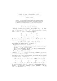
Chapter 5Applications of second-order ODEsContents5.1 Resonant electric circuits . . . . . . . . . . . . . . . . . . . . 775.2 Further applications . . . . . . . . . . . . . . . . . . . . . . . 805.1 Resonant electric circuitsA resonant electric circuit (or LRC circuit) consists of an imposed voltage E(t), andthree circuit elements: an inductor, a resistor and a capacitor:I(t)V Inductor = L dIdtE(t)V Resistor = IRdV Capacitordt= 1 C IKirchhoff’s Circuit Laws state that the current I(t) is the same through each element,and that the sum of the voltages across each element is equal to the imposed voltageE(t).Voltages are measured in Volts, currents (I) in Amperes, charge (Q) in Coulombs,inductance (L) in Henrys, resistance (R) in Ohms, and capacitance (C) in Faradays.77

78 5.1 Resonant electric circuitsVoltage drop across an inductanceVoltage drop across a resistorVoltage drop across a capacitorV Inductor = L dIdt .V Resistor = IR.V Capacitor = 1 C Q,where Q is the charge in the capacitor (related to the current by I = dQ/dt), sodV Capacitordt= 1 C I.The sum of the three voltages equals the imposed E(t):V Inductor + V Resistor + V Capacitor = E(t).Differentiate and substitute the three relations above:L d2 Idt + RdI2 dt + 1 C I = dEdtWe will solve this in the case of an imposed sinusoidal voltage of amplitude E 0 andfrequency ω, that is, E(t) = −E 0 cos ωt:L d2 Idt 2 + RdI dt + 1 C I = ωE 0 sin ωt.First, we find the characterstic equation by substituting I = e λt into the homogeneousequation, and dividing by e λt :The roots are:Lλ 2 + Rλ + 1 C = 0, or LCλ2 + RCλ + 1 = 0,λ = −RC ± √ R 2 C 2 − 4LC.2LCWhen LRC circuits are used as resonant electric circuits, the resistance R is small, sothe roots are complex. Let the roots be√λ = −α ± i ω0 2 − α 2 ,whereα = R 2L

Chapter 5 – Applications of second-order ODEs 79is called the attenuation factor andω 0 = 1 √LCis the (undamped) resonant frequency. Thus the Complementary Function isI CF = e −αt (C 1 cos(ω d t) + C 2 sin(ω d t)) .with ω d = √ ω 2 0 − α 2 being the damped resonant frequency. Note that since α > 0, wehave I CF → 0 as t → ∞.Now we look for a Particular Integral:I P I = A cos(ωt) + B sin(ωt).Before proceeding, divide the ODE by L and use α and ω 0 to eliminate L and R:LC = ω0 −2 and RC = 2αω0 −2 :d 2 Idt + 2αdI2 dt + ω2 0I = ω E 0sin ωt.LSubstitute the assumed form of the Particular Integral into the ODE:(−Aω 2 + 2Bαω + Aω 2 0)cos(ωt) +(−Bω 2 − 2Aαω + Bω 2 0)sin(ωt) = ωE 0Lsin ωtCompare terms multiplying cos(ωt) and sin(ωt) to get a pair of equations for A andB:−Aω 2 + 2Bαω + Aω0 2 = 0 and − Bω 2 − 2Aαω + Bω0 2 = ω E 0L ,which can be solved:A = − E 0L2αω 2and B = E 0(ω 2 − ω0) 2 2 + 4α 2 ω 2 Lω(ω 2 − ω 2 0)(ω 2 − ω 2 0) 2 + 4α 2 ω 2 .The Particular Integral I P I = A cos(ωt) + B sin(ωt) can also be written in the formI P I = √ A 2 + B 2 sin(ωt + arctan(A/B))(elementary trigonometry), so we call √ A 2 + B 2 the amplitude of I P I :√A2 + B 2 = E 0Lω√(ω2 − ω 2 0) 2 + 4α 2 ω 2 .The general solution is I CF + I P I , but since I CF → 0 as t → ∞, only I P I remains afterI CF has decayed away. As a function of ω, this is maximum at ω = ω 0 .We can plot the amplitude of I P I as a function of ω in the case (for example) L = 1 H,R = 2 Ω and C = 0.5 F, with E 0 = 1 V, so the original ODE isd 2 Idt 2 + 2dI dt+ 2I = ω sin ωt,

80 5.2 Further applications(roots are −1 ± i) andIn this case, the amplitude of I P I is√A2 + B 2 =α = 1 and ω 0 = √ 2.ω√4ω2 + (ω 2 − 2) 2 =ω√ω4 + 4√A2 + B 20.51 2 3 4 5 6 7 8 9 10As a second example, take R = 0.2 Ω but otherwise the same as the first example. Inthis case, α = 0.1 and√ 5ωA2 + B 2 = √25ω4 − 99ω 2 + 100ω√A2 + B 25ω1 2 3 4 5 6 7 8 9 10With smaller α, the peak of the response is much more sharply focussed at ω = ω 0 .This forms the basis of a band pass filter: the circuit responds only frequencies closeto ω 0 . LRC circuits are used as tuners in simple radio receivers.5.2 Further applicationsSimple supply/demand/price models; Voting model; Modelling infectious diseases; Twospecies radioactive decay; Gradient systems.