On the optimal design of structured feedback gains - LC Smith ...

On the optimal design of structured feedback gainsfor interconnected systemsMakan Fardad, Fu Lin, and Mihailo R. JovanovićAbstract— We consider the design of optimal static feedbackgains for interconnected systems subject to architectural constraintson the distributed controller. These constraints are inthe form of sparsity requirements for the feedback matrix,which means that each controller has access to informationfrom only a limited number of subsystems. We derive necessaryconditions for the optimality of structured static feedbackgains in the form of coupled matrix equations. In generalthese equations have multiple solutions, each of which is astationary point of the objective function. For stable open-loopsystems, we show that in the limit of expensive control, theoptimal controller can be found analytically using perturbationtechniques. We use this feedback gain to initialize homotopybasedgradient and Newton iterations that find an optimalsolution to the original (non-expensive) control problem. Forunstable open-loop systems, the centralized truncated gain isused as an initial estimate for the iterative schemes aimed atfinding the optimal structured feedback gain. We consider bothspatially invariant and spatially varying problems and illustrateour developments with several examples.Index Terms— Architectural constraints, interconnected systems,optimal decentralized control, structured feedback gains.I. INTRODUCTIONLarge-scale systems are ubiquitous in nature and in modernengineering applications. The individual componentsof a large-scale system are often equipped with sensing,computation, and actuation capabilities. A central questionin the control of such systems then becomes, what is a goodcommunication architecture between the controllers of thedifferent subsystems? Clearly there is a trade-off in play: thebest possible performance is attained if all controllers cancommunicate to each other, and as a whole decide uponthe control action to be applied to each subsystem. This,however, comes at the expense of excessive communicationand computation requirements. The other extreme is whenevery controller acts in isolation, and applies a controlaction to its corresponding subsystem based on its ownmeasurement of the subsystem’s output. This scenario placesminimum communication and computation requirements onthe controllers, but generally comes at the expense of poorperformance.A desired scenario, and a reasonable middle ground, is thelocal communication of subsystems with their immediate ornearest neighbors, referred to as localized control. It is thistype of decentralized control that is the focus of the presentresearch effort.Financial support from the National Science Foundation under CAREERAward CMMI-06-44793 and under Award CMMI-09-27720 is gratefullyacknowledged.M. Fardad is with the Department of Electrical Engineering and ComputerScience, Syracuse University, NY 13244. F. Lin and M. R. Jovanovićare with the Department of Electrical and Computer Engineering, Universityof Minnesota, Minneapolis, MN 55455. E-mails: makan@syr.edu,fu@umn.edu, mihailo@umn.edu.The synthesis problem of distributed control for interconnectedsystems has received considerable attention inrecent years [1]–[14]. For linear spatially invariant plants,it was shown in [1] that optimal controllers are themselvesspatially invariant. Furthermore, for optimal distributed problemswith quadratic performance indices the dependenceof a controller on information coming from other parts ofthe system decays exponentially as one moves away fromthat controller [1]. These developments motivate the searchfor inherently localized controllers. For example, one couldsearch for optimal controllers that are subject to the conditionthat they communicate only to other controllers within acertain radius. However, the framework of [1] does not allowthe a priori specification of the communication architectureof the distributed controller. Additionally, it does not provideerror bounds on the deviation from optimality if one wereto truncate the information dependence of every controller,for example by confining it to communicating within a prespecifiedradius of itself.Thus the problem of controller design for large-scale anddistributed systems is mostly dominated by the architecturaland localization constraints imposed on the controller. Suchdesign problems are well-known to be difficult, with almostthree decades of research in an area that has come to beknown as the ‘decentralized control of large-scale systems’;see [15] and references therein.A problem of wide interest is to search for an optimaldistributed controller that is a static gain (i.e., has no temporaldynamics) with a priori assigned localization constraints.Such controllers are less sophisticated than dynamic controllers,and thus may achieve lower performance, but havethe advantage of being much easier to implement. Mostarchitectural requirements on the distributed static controllerare in the form of sparsity constraints. We focus particularlyon cases where the static feedback gain can be partitionedinto banded matrices, which are non-zero only on the maindiagonal and a relatively small number of sub-diagonals.Such banded structure translates to each controller using onlylocal information to compute the control action. We searchfor structured controllers that minimize the H 2 norm. We finda coupled set of algebraic matrix equations that characterizenecessary conditions for the optimality of the structured staticcontroller.The challenging aspect of solving the aforementionedcoupled equations is that they can have multiple solutions,each of which is a stationary point of the norm minimizationproblem. In general, it is not known how many local minimaexist or how to find them. For stable open-loop systems, weconsider the case of expensive control [16] in which a perturbationanalysis of the necessary conditions for optimalitycan be performed. The expensive control scenario restrictsthe norm of the distributed gain as it tries to minimize

the use of control effort. Perturbation analysis results inequations that are decoupled and thus readily solvable tofind expansion terms of arbitrarily high-order. This leadsto a unique optimal gain that is small in norm; this gaincan be used to initialize a homotopy-based gradient andNewton iterations to determine optimal controller for smallervalues of control penalty. In this numerical scheme thelevel of expensiveness of the control problem is successivelyreduced and the resulting matrix equations are solved untilthe original (non-expensive) control objective is recovered.For unstable open-loop systems, we apply a spatial truncationon the optimal centralized feedback gain to initialize aniterative numerical scheme that is aimed at solving necessaryconditions for optimality subject to structural constraints.An interesting example of this procedure arises in the caseof spatially invariant systems; for such systems the optimalstatic feedback is a centralized gain whose spatial dependencedecays exponentially with distance [1]. We thereforeexpect that the truncated gain would be a reasonable initialestimate for the Newton-based iterative scheme that attemptsto find the optimal structured feedback gain.The paper is organized as follows: in Section II thestructured optimal control problem is formulated and necessaryconditions for optimality are found. In Section IIIwe consider stable open-loop systems and apply a perturbationanalysis on these necessary conditions to find theunique optimal expensive static controller. In Section IVgradient- and Newton-based iterative schemes are used tofind stabilizing (locally) optimal distributed controllers. InSection V we provide illustrative examples, and in Section VIwe summarize our developments.II. NECESSARY CONDITIONS FOR OPTIMALITYConsider the control problem˙ψ = A ψ + B 1 w + B 2 u,z = C 1 ψ + D u,y = C 2 ψ, u = −F y,where C 1 = [ Q 1/2 0 ] ∗ [ ]and D = 0 R1/2 ∗. Thematrix F denotes the static feedback gain which is subject tostructural constraints. Specifically, the structural constraintsdictate the zero entries of the feedback gain. We assume thatthe subspace S encapsulates these constraints and that thereis a stabilizing F ∈ S.Upon closing the loop, the above problem can equivalentlybe written as˙ψ = (A − B 2 F C 2 ) ψ + B 1 w,[]Qz =1/2(H2)−R 1/2 ψ.F C 2Note that w denotes exogenous signals and that the performanceoutput z encapsulates both the amplitude of the stateand that of the control input. We now consider the followingoptimal control problem:• Find the matrix F ∈ S such that ‖H‖ 2 2 is minimized,where H is the transfer function from w to z and ‖ · ‖ 2is the H 2 norm.It can be shown [17] that this optimal control problem isequivalent tominimize J = trace (P B 1 B ∗ 1)subject to (A − B 2 F C 2 ) ∗ P + P (A − B 2 F C 2 )= − (Q + C ∗ 2 F ∗ RF C 2 ) , F ∈ S.(SG)Note that the first constraint in (SG) is nothing but theLyapunov equation A ∗ cl P + P A cl = −C ∗ cl C cl correspondingto the closed-loop system (H2). We remark that – when thereare no structural constraints on F – the above problem isstrongly related to the static output-feedback LQR problemconsidered in [18].Most structural requirements on the gain F are in theform of sparsity constraints. A sparse matrix is populatedprimarily with zeros and the pattern of the non-zero entriesdescribes the communication architecture of the distributedcontroller; if the ijth block of F is non-zero it means thatsubsystem j is communicating its state to the controller ofthe ith subsystem. We focus particularly on cases whereF is a banded matrix, i.e., it is only non-zero on its mainblock-diagonal and a relatively small number of block subdiagonals.For vehicular platoons, such a banded structuretranslates to each vehicle using only information aboutthe position and velocity of a relatively small number ofneighboring vehicles to control its own position and velocity.Theorem 1 (Necessary conditions for optimality):In order for matrix F ∈ S, with A − B 2 F C 2 Hurwitz, to beoptimal for the problem (SG) it is necessary that it satisfiesthe following set of equations:(A − B 2 F C 2 ) ∗ P + P (A − B 2 F C 2 )= − (Q + C ∗ 2 F ∗ RF C 2 ) , (NC1)(A − B 2 F C 2 ) L + L (A − B 2 F C 2 ) ∗ = −B 1 B ∗ 1, (NC2)(RF C 2 LC ∗ 2 ) ◦ I S = (B ∗ 2P LC ∗ 2 ) ◦ I S , (NC3)where ◦ denotes the element-wise multiplication of matricesand the matrix I S is defined as{ 1 if Fij is a free variable,[I S ] ij=0 if F ij = 0 is required.Remark 1: Similar necessary conditions for optimality offixed-order dynamic controllers appear in [19]. To differentiateour results from those of [19], we note that the equivalentof equation (NC3) in [19] is given in the form of summationof matrix multiplications, which is much more expensive tocompute than (NC3). Further, for stable open-loop systemswe develop homotopy-based descent method by utilizingthe perturbation analysis in the limit of expensive control.Also, the Newton direction for the design of static structuredfeedback gains is determined for the first time in our work.We consider (NC3) for a few important examples of S:• S is the subspace of diagonal matrices. In this caseI S = I. The optimality condition (NC3) becomes(RF C 2 LC ∗ 2 ) ◦ I = (B ∗ 2P LC ∗ 2 ) ◦ I,which can also be written as diag {RF C 2 LC ∗ 2 } =diag {B ∗ 2P LC ∗ 2 }.• S is the subspace of tridiagonal matrices. In this caseI S = T , where T is the tridiagonal matrix with elementsequal to one on the main diagonal, first upper, and firstlower subdiagonals. The optimality condition (NC3)

O(1) : F (0) = 0⎧⎪⎨ A ∗ P (0) + P (0) A = −QO(ε) :⎪⎩⎧⎪⎨O(ε 2 ) :⎪⎩.AL (0) + L (0) A ∗ = −B 1 B1∗F (1) = ([B2P ∗ (0) L (0) C2 ∗ ] ◦ I) ([C 2 L (0) C2 ∗ ] ◦ I) −1A ∗ P (1) + P (1) A = (B 2 F (1) C 2 ) ∗ P (0) + P (0) (B 2 F (1) C 2 ) − C ∗ 2 F (1)∗ F (1) C 2AL (1) + L (1) A ∗F (2)= (B 2 F (1) C 2 ) L (0) + L (0) (B 2 F (1) C 2 ) ∗= ([B ∗ 2P (0) L (1) C ∗ 2 + B ∗ 2P (1) L (0) C ∗ 2 − F (1) C 2 L (1) C ∗ 2 ] ◦ I) ([C 2 L (0) C ∗ 2 ] ◦ I) −1.(EXP)either the negative gradient direction, F d = −F g , or theNewton direction, F d = F nt , we next employ the standardbacktracking line search, with parameters α = 0.3 andβ = 0.5 (see [21, p. 464]), to determine the step-size. Inaddition to providing decrease in J, it is also necessary toguarantee the closed-loop stability when selecting the stepsize.Hence, given descent direction F d and step-size s = 1:Stepsize searchrepeat: s := βsuntil: both conditions are satisfied1) J(F + sF d ) < J(F ) + α s trace(∇J(F ) T F d );2) A cl = A − B 2 (F + sF d )C 2 is Hurwitz.Iterative algorithmGiven a stabilizing F 0 , the iterative algorithm at each stepk is given by1) compute descent direction F d (F k );2) use step-size search to determine s k ;3) update F k+1 = F k + s k F d (F k ).until: stopping criterion ‖∇J(F k )‖ 2 < ɛ is reached.C. Homotopy-based iterationsFor stable open-loop systems, the design procedure of SectionIII can be extended to non-expensive control regimes viathe use of homotopy (i.e., continuation) methods. Homotopymethods are based on replacing the problem of interest by aparameterized family of problems with following properties:(i) the problem is easily solved for small values of theparameter; and (ii) as the parameter value is increased theproblem transforms into the problem of interest.We thus consider the following iterative scheme to find theoptimal structured F that solves optimization problem (SG).Let R = (1/ε) I, where ε is a positive scalar and I isthe identity matrix. Treating ε as the homotopy parameter,we first find the optimal structured F that minimizes (SG)for very small values of ε. This has the interpretation ofexpensive control [16]; a small ε results in a large R, whichin light of the output matrix in (H2) means that controleffort has to be spent sparingly. The solution of this problemresults in a structured feedback gain F that is small in normand is computed easily and reliably using MATLAB (for verysmall ε, the matrix F can be computed using the perturbationanalysis of Section III). We now slightly increase the valueof ε and use the obtained F to initialize the next roundof gradient or Newton iterations. We continue increasingthe value of ε until the matrix R of the original controlobjective is recovered. This algorithm effectively guides theoptimization scheme through the many local minima.V. EXAMPLESA. Spatially varying mass-spring systemIn this section we revisit a mass-spring system on a linedescribed in Example 1. The centralized optimal controller,u = −Kψ, is given by K = R −1 B ∗ 2X, where X is thepositive definite solution of the algebraic Riccati equationA ∗ X + XA + Q − XB 2 R −1 B ∗ 2X = 0.The initial feedback gain F 0 is determined by projecting Konto the information structure S, that isF 0 = [ F 0p F 0v ] = K ◦ [ S p I ].It turns out that F 0 for any p ≥ 0 is a stabilizing feedbackgain. Thus, the iterative descent algorithm of Section IV-Acan be initialized with F 0 . We note that other approacheshave been developed to find a stabilizing feedback gain [7].The stopping criterion for the algorithms is ‖∇J(F )‖ 2

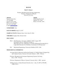
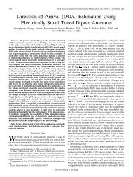
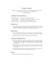
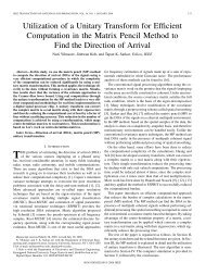
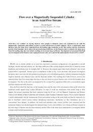
(a)Fig. 2. Comparison of elements on the main diagonals of: (a) initial andoptimal position feedback gains; (b) initial and optimal velocity feedbackgains. Mass-spring system of Example 1 with {p = 1, N = 50, Q = I,R = 10I} is considered.(a)Fig. 3. Scaling of ‖ ¯H‖ 2 2 := (1/N)‖H‖2 2 with the number of vehiclesN for: (a) truncated optimal centralized controller (dashed) and structuredcontroller (solid) with spatial spread p = 4; (b) structured (with spatialspread p = {1, 2, 3, 4}) and centralized state-feedback controllers.B. System of single integrator vehicles on circleWe next consider the design of structured controllersof spatial spread p for a system of identical single integratorvehicles described in Example 2 with C 2θ =[ 2 (1 − cos (2πθ/N)) · · · 2 (1 − cos (2πp θ/N)) ] ∗ , F =[ f 1 · · · f p ] , and the following pair of state/control weights(Q θ , r) = (2 (1 − cos (2πθ/N)) , 1). The selected statepenalty accounts for the difference between the position ofvehicle n and the average of positions of two neighboringvehicles. In this case, the optimal centralized state-feedbackcontroller, u θ = −K θ ψ θ , is given by K θ = Q 1/2θ, and the optimalstructured controller with p = 1 is given in Example 2.To determine the structured controller with p ≥ 2, we applyNewton’s method to solving (NC’) by initiating the iterationswith a truncated centralized controller. Figure 3(a) illustratesthe performance comparison of the truncated centralized controllerand the structured controller with spatial spread p = 4;clearly, Newton’s iteration provides appreciable performanceimprovement relative to the truncated centralized controller.The performance of structured controllers with spatial spreadp = {1, 2, 3, 4} (obtained by applying Newton’s methodto (NC’)) and optimal centralized controller is shown inFig. 3(b). As expected, an increase in the spatial spreaddecreases the performance gap between optimal structuredand optimal centralized designs.VI. CONCLUSIONSWe study the static H 2 synthesis problem subject to thefeedback gain satisfying certain sparsity constraints. Theseconstraints are such that they enforce a localized communicationarchitecture between the underlying plant and thecontroller. We find necessary conditions for optimality of(b)(b)localized controllers that are in the form of coupled matrixequations. In general these equations have multiple solutions,which correspond to different stationary points. However, forstable open-loop systems, in the limit of expensive control,perturbation methods can be used to find a unique optimalcontroller. We use this controller to initialize a homotopybasednumerical optimization scheme that determines optimalcontroller in the non-expensive regime. For unstableopen-loop systems, an iterative scheme utilizing gradientand Newton’s methods is employed to determine a solutionto stationary conditions for optimality. The iterations areinitialized by projecting optimal centralized controllers tothe set of controllers with desired localization properties.The presented algorithms appear to work well in practiceas demonstrated by illustrative examples in Section V.REFERENCES[1] B. Bamieh, F. Paganini, and M. A. Dahleh, “Distributed control ofspatially invariant systems,” IEEE Trans. Automat. Control, vol. 47,no. 7, pp. 1091–1107, 2002.[2] G. A. de Castro and F. Paganini, “Convex synthesis of localizedcontrollers for spatially invariant system,” Automatica, vol. 38, pp.445–456, 2002.[3] P. G. Voulgaris, G. Bianchini, and B. Bamieh, “Optimal H 2 controllersfor spatially invariant systems with delayed communicationrequirements,” Syst. Control Lett., vol. 50, pp. 347–361, 2003.[4] R. D’Andrea and G. E. Dullerud, “Distributed control design forspatially interconnected systems,” IEEE Trans. Automat. Control,vol. 48, no. 9, pp. 1478–1495, 2003.[5] G. Dullerud and R. D’Andrea, “Distributed control of heterogeneoussystems,” IEEE Trans. Automat. Control, vol. 49, no. 12, pp. 2113–2128, December 2004.[6] C. Langbort, R. S. Chandra, and R. D’Andrea, “Distributed controldesign for systems interconnected over an arbitrary graph,” IEEETrans. Automat. Control, vol. 49, no. 9, pp. 1502–1519, September2004.[7] V. Gupta, B. Hassibi, and R. M. Murray, “On the synthesis of controllaws for a network of autonomous agents,” in Proceedings of the 2004American Control Conference, 2004, pp. 4927–4932.[8] B. Bamieh and P. G. Voulgaris, “A convex characterization of distributedcontrol problems in spatially invariant systems with communicationconstraints,” Syst. Control Lett., vol. 54, pp. 575–583, 2005.[9] M. Rotkowitz and S. Lall, “A characterization of convex problems indecentralized control,” IEEE Trans. Automat. Control, vol. 50, no. 12,pp. 1984–1996, 2005.[10] A. Rantzer, “Linear quadratic team theory revisited,” in Proceedingsof the 2006 American Control Conference, 2006, pp. 1637–1641.[11] ——, “A separation principle for distributed control,” in Proceedingsof the 45th IEEE Conference on Decision and Control, 2006, pp. 3609–3613.[12] N. Motee and A. Jadbabaie, “Optimal control of spatially distributedsystems,” IEEE Trans. Automat. Control, vol. 53, no. 7, pp. 1616–1629, Aug. 2008.[13] F. Borrelli and T. Keviczky, “Distributed LQR design for identical dynamicallydecoupled systems,” IEEE Trans. Automat. Control, vol. 53,no. 8, pp. 1901–1912, Sept. 2008.[14] M. Fardad and M. R. Jovanović, “On the state-space design of optimalcontrollers for distributed systems with finite communication speed,”in Proceedings of the 47th IEEE Conference on Decision and Control,2008, pp. 5488–5493.[15] D. D. Šiljak, Decentralized Control of Complex Systems. AcademicPress, 1991.[16] T. Kailath, Linear Systems. Prentice Hall, 1979.[17] K. Zhou, J. Doyle, and K. Glover, Robust and Optimal Control.Prentice Hall, 1996.[18] W. S. Levine and M. Athans, “On the determination of the optimalconstant output feedback gains for linear multivariable systems,” IEEETrans. Automat. Control, vol. 15, no. 1, pp. 44–48, 1970.[19] C. J. Wenk and C. H. Knapp, “Parameter optimization in linear systemswith arbitrarily constrained controller structure,” IEEE Trans. Automat.Control, vol. 25, pp. 496–500, 1980.[20] D. P. Bertsekas, Nonlinear programming. Athena Scientific, 1999.[21] S. Boyd and L. Vandenberghe, Convex Optimization. CambridgeUniversity Press, 2004.[22] R. A. Horn and C. R. Johnson, Topics in Matrix Analysis. CambridgeUniversity Press, 1994.