Boundary value problems 1 Introduction 2 Boundary conditions

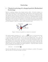
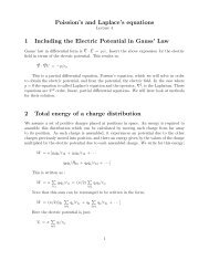
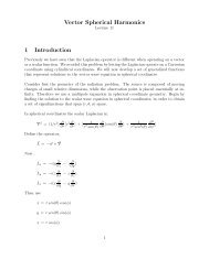
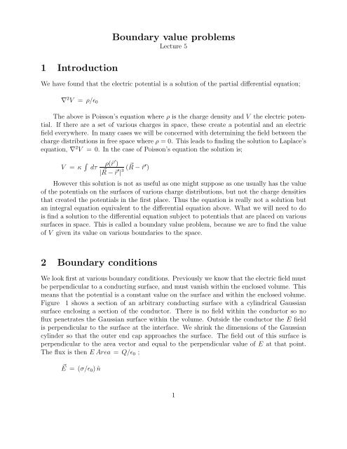
1 IntroductionBoundary value problemsLecture 5We have found that the electric potential is a solution of the partial differential equation;∇ 2 V = ρ/ǫ 0The above is Poisson’s equation where ρ is the charge density and V the electric potential.If there are a set of various charges in space, these create a potential and an electricfield everywhere. In many cases we will be concerned with determining the field between thecharge distributions in free space where ρ = 0. This leads to finding the solution to Laplace’sequation, ∇ 2 V = 0. In the case of Poisson’s equation the solution is;V = κ ∫ dτρ(ˆr ′ )| ⃗ R − ⃗r ′ | 3 (⃗ R − ⃗r ′ )However this solution is not as useful as one might suppose as one usually has the valueof the potentials on the surfaces of various charge distributions, but not the charge densitiesthat created the potentials in the first place. Thus the equation is really not a solution butan integral equation equivalent to the differential equation above. What we will need to dois find a solution to the differential equation subject to potentials that are placed on varioussurfaces in space. This is called a boundary value problem, because we are to find the valueof V given its value on various boundaries to the space.2 Boundary conditionsWe look first at various boundary conditions. Previously we know that the electric field mustbe perpendicular to a conducting surface, and must vanish within the enclosed volume. Thismeans that the potential is a constant value on the surface and within the enclosed volume.Figure 1 shows a section of an arbitrary conducting surface with a cylindrical Gaussiansurface enclosing a section of the conductor. There is no field within the conductor so noflux penetrates the Gaussian surface within the volume. Outside the conductor the E fieldis perpendicular to the surface at the interface. We shrink the dimensions of the Gaussiancylinder so that the outer end cap approaches the surface. The field out of this surface isperpendicular to the area vector and equal to the perpendicular value of E at that point.The flux is then E Area = Q/ǫ 0 ;⃗E = (σ/ǫ 0 ) ˆn1

dlEn^σEn^En^Figure 1: The geometry required to use Gauss’ law and Ampere’s law to determine theboundary conditions at a conducting surface.where σ is the surface charge density and ˆn is the outward normal. Then the surfacecharge on a conductor is given by;σ = −ǫ 0⃗ ∇V · ˆnThe above technique will also be useful to develop the boundary condition at nonconductingsurfaces, so it will be revisited later. We already know that the electric fieldtangent to a conducting surface vanishes. We now look at this more closely. In figure 1there is a drawing of a closed loop that encloses the surface. This loop is called an Amperianloop and we apply reasoning similar to that used above. In this case we consider thecirculation, Γ, of the field around the loop as the loop is reduced to lie near, both above andbelow, the surface. Thus contributions to the circulation from the edges of the loop vanishas the side length approaches zero. This leaves the result;Γ = E ‖ above dl − E ‖ below dlFor static charge Γ = 0 so that E ‖ above = E ‖ below , and for a conductor both equal zero.As with the Gaussian surface, this will be useful later and will be revisited at that time.3 UniquenessWe will be looking for solutions to a second order partial differential equation. This solutioncan be determined in several ways, and will usually be represented in the form of a seriesof special functions obtained from the solutions to a set of eigenvalue equations. Thus thesolution may take different forms, and an important question will arise. How do we knowthat the solution we find is unique? After all, a proper physics solution should have onlyone answer, ( one numerical value when evaluated). There are mathematical proofs that2

unique solutions to various second order differential equations have a unique solution if theysatisfy the differential equation and also have a specified value on a set of boundaries in thegeometric space in which the equation applies. These conditions are specified in table 1,and finding a proper solution is called a boundary value problem.Table 1: Boundary conditions required for unique solutions to various2 nd order partial differential equationsPoisson’s Eqn Wave Eqn Diffusion Eqn∇ 2 V = ρ/ǫ ∇ 2 V = (1/c 2 ) ∂2 V∂t 2 ∇ 2 V = (1/a) ∂V∂tDirichletOpen Surface not enough not enough uniqueClosed Surface unique too much too muchNeumannOpen Surface not enough not enough uniqueClosed Surface unique too much too muchCauchyOpen Surface unstable unique too muchClosed Surface too much too much too muchThe Dirichlet boundary conditions require specification of the value of the solution onthe boundary. The Neumann boundary conditions require the specification of the derivativeof the solution on the boundary. The Cauchy boundary conditions require the specificationof both the value of the solution and its normal derivative on the boundary. Here we areinterested in the solution to Laplace’s (or Poisson’s) equation which requires specification ofthe value of the solution (or ) its derivative on a closed surface. Later we consider the waveequation (hyperbolic equation form) when we study dynamics.As a very simple example here we write the potential between the plates of a parallelplate capacitor as;V = −V 0 (z/d) + constantHere d is the distance between the plates and z is the coordinate in this direction sothat z = constant represents the potential on lower plate and z = d the potential on theupper one. By this we have satisfied the boundary condition that ⃗ E is perpendicular tothe plates. This is a Neumann condition applied on a closed boundary. The space betweenthe plates which extends to ∞ in both directions in (x, y). The function also satisfies3

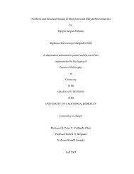
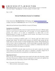
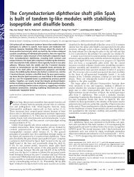
d−qE++ ++ ++V = 0+EE+q−dImage ChargeFigure 2: An image charge solution for a charge,−q above an infinite conducting plane. Weobtain the field at the point P.Laplace’s equation, so by the uniqueness theorem, this is the unique solution to the problem.4 ImagesNow that we have a uniqueness theorem we can attempt to find solutions by applying symmetriesto guess a solution. Then if the uniqueness theorem is satisfied we have found a truerepresentation of the solution. We first take as an example the solution of a point charge,−q, above an infinite conducting plane. This is shown in figure 2. In this example thereis no field below the (x, y) conducting plane. The boundary conditions are that the field(normal derivative of the potential) must be perpendicular to the plane, the field at the pointmust be given by Coulomb’s law, and the field at infinity must decrease to zero. This formsa closed surface within which we are to find the potential and the field. The uniquenesstheorem states that if we specify either the value of the potential or its derivative on thissurface we obtain the unique solution to the problem. To do this we remove the conductingplane and replace it by an image charge as shown in figure 2. Note that by doing this thefield is perpendicular to the (x, y) plane, and it has the form of Coulomb’s law as it getsclose to the charge, q. It also satisfies the boundary condition at z → ∞. This must givethe solution we seek for z ≥ 0. Of course we must ignore the solution for z < 0 where wealready know that the field must vanish. The solution for the potential at point, P is;V = κ q[1|⃗r + d| ⃗ − 1|⃗r − d| ⃗ ]The field is then obtained by ⃗ E = − ⃗ ∇V . We also see that when ⃗r = 0 the evaluation point4

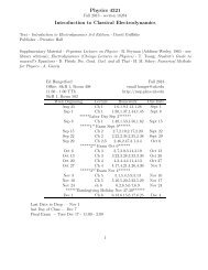
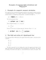
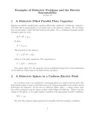
qrq’r’z’zV = 0Figure 3: An image charge solution for a charge,q outside a conducting spherical shelllies on the conducting surface and the potential equals zero.Now consider a point charge above a conducting spherical surface. In this example wewant to remove the surface and replace it by an image charge so that the potential on thespherical surface has a constant value of zero. This is shown in figure 3. In the imageproblem we have a charge q a distance of z 1 > R above the center of the sphere, and −q ′ adistance z ′ < R from the center of the sphere. Then we evaluate the potential at a point, ⃗r,on the spherical surface which we must force to be zero.qV = κ[|⃗z − ⃗r| − q′|⃗r − ⃗z| ]Then we write;q|⃗z − ⃗r| = (q z ) 1[1 + (r/z) 2 − 2(r/z) cos(θ)] 1/2q ′|⃗r − ⃗z ′ | = (q′ r ) 1[1 + (z ′ /r) 2 − 2(z ′ /r) cos(θ)] 1/2For these 2 terms to cancel we must choose;q/z = −q ′ /r and r/z = z ′ /rTherefore we choose the image to be placed at;z ′ = z/r 2 and q ′ = −(r/z)q5

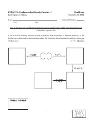
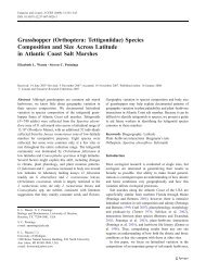
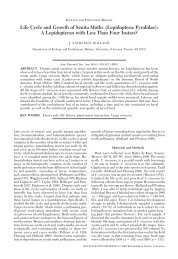
d dra’−λ aλrwV = −V 0V = V 0wFigure 4: An image charge solution for two conducting cylinders held at opposite potentialsFinally look at figure 4. This represents two infinite, conducting cylinders which arechosen to have potentials V 0 and −V 0 on their surfaces. We want to find the potential everywherein space, and to do this we can apply the method of images. We replace the cylindersby image line charges λ and −λ as shown. This problem can be worked in the 2-D of thefigure because of the symmetry. Recall that the potential of a line charge is;V =λ2πǫ 0ln(a)Here a is the distance from the line charge to the field point, P. From the figure, thepotential at the position of the cylindrical surface of the left cylinder is;V T =λ2πǫ 0[ln(a) − ln(a ′ )] =λ2πǫ 0[ln(a/a ′ )]From the location of the center point of the left cylinder;⃗r ′ = ⃗w +⃗a ′ and ⃗a ′ = ⃗r ′ − ⃗w⃗r ′ =Then;2d⃗− w +⃗a and ⃗a = ⃗r ′ − 2d ⃗ − wa ′ 2 = r ′ 2 + w 2 − 2r ′ w cos(θ) = r ′2 [1 + (w/r ′ ) 2 − 2(w/r ′ ) cos(θ)]a 2 = r ′ 2 +(2d −w) 2 −2r ′ (2d −w) cos(θ) = (2d −w) 2 [1+(r ′ /(2d −w)) 2 −2(r ′ /(2d −w)) cos(θ)]Substitution gives for the potential givesV T =λ2πǫ 0[ln[(2d − w)/r ′ ]6

(1/2) ln[ 1 + (r′ /(2d − w)) 2 − 2(r ′ /(2d − w)) cos(θ)1 + (w/r ′ ) 2 − 2(w/r ′ ])cos(θ)The second term on the right vanishes if;(r ′ /(2d − w)) = w/r ′w = d ± √ d 2 − r ′The potential over the cylinder defined by the radius r ′ is a constant value given by;V T =λ2πǫ 0[ln[(2d − w)/r ′ ]The potential on the right cylindrical surface is the negative on this value.5 Separation of VariablesWe wish to find a solution to Laplace’s equation which is a 2 nd order, linear, homogeneous,partial differential equation. The standard technique for finding a solution to this type ofequation is to use separation of variables. That is to assume a solution in the form ofX(x)Y (y)Z(z) - a product of separate functions of x and,y, and z. Clearly not all solutionscan be put in this form. The technique is useful if there is a coordinate system that canmatch the boundaries of the problem. That is if surfaces of a constant variable are thesurfaces on which the boundary conditions are applied. Thus the solution can at least beplaced in separable form at the boundary. For Laplace’s equation the possibility of obtaininga separable solution occurs for a small number of coordinate systems. These are listed intable 2. However, just because a separable solution can be found does not mean separableboundary conditions are possible.There are a few other systems not listed in the table that allow R separation, whichbasically means they separate for one or two of the variables. We found a solution by imagesfor a system of two long conducting cylinders. This system can be defined in Bi-cylindricalCoordinates which is R separable. Such coordinates can be used if symmetry can be appliedto automatically remove one or two of the coordinate variables from the solution. In theBi-cylindrical coordinates, (r, θ, z), separation occurs when the solution is independent ofz, see figure 5. All of the coordinate systems listed in the table are 3-dimensional andorthogonal. However, in this course we deal with only Cartesian, Circular Cylindrical, andSpherical coordinates.When separation of variables is applied, one obtains a set of 2 nd order ordinary differ-7

Table 2: Coordinate systems in which Laplace’s equation separates. To find a solution onemust apply the boundary condition on a surface defined when one variable is constant.Coordinate System VariablesCartesian Coordinates (x,y,z)Circular Cylindrical Coordinates (r, φ, z)Elliptic Cylindrical Coordinates (η, φ, z)Parabolic Cylindrical Coordinates (µ, φ, z)Spherical Coordinates (r, θ, φ)Prolate Spheroidal Coordinates (η, θ, φ)Oblate Spheroidal Coordinates (η, θ, φ)Parabolic Spheroidal Coordinates (µ, θ, φ)Conical Coordinates (r, θ, λ)Ellipsoidal Coordinates (r, θ, λ)Paraboloidal Coordinates (µ, ν, λ)ential equations (ode) of the form;ddz [p(z)dη ] + [q(z) + λ r(z)]η = 0dzhere λ is a constant of separation and p, q, r are functions which depend on the coordinatesystem. The solution which represents a specific physical problem occurs by applyingthe boundary conditions. This specifies a discrete but infinite set of the separation constants,λ n and solutions η n (z). The solution to the ode we seek can then be constructed from thisset of functions. The problem of finding a solution to the ode subject to boundary conditionsis called the Sturm-Liouville problem.6 The Sturm-Liouville ProblemThe Sturm-Liouville solutions are eigenfunctions and the value of λ n are the correspondingeigenvalues. These functions form an orthogonal set of functions in the space defined withinthe problem boundaries, a ≤ z ≤ b. We have visited this previously. Thus any function,F(z), can be represented by a linear sum of eigenfunctions;F(z) = ∞ ∑so that;n=0A n η n (z)lim m→∞∫badz [F(z) − m ∑n=0A n η n (z)] 2 r(z) = 08

Figure 5: The geometry of Bi-cyclindrical coordinates which is R separableThis represents convergence in the mean. In addition;∫dz r(z) ηn (z) η m (z) = 0 when m ≠ n and(λ n − λ m ) ≠ 0So that the eigenfunctions are orthogonal using a weighting factor r(z) which comesfrom the above ode.7 Example in Cartesian CoordinatesA simple example illustrates the eigenvalue solution to the ode which is used to find a representationto the function F(z) given in figure 6. We seek a solution to the equation belowin Cartesian Coordinates ;d 2 ηdz + λ η = 0Comparison to the ode of the general Sturm-Liouville problem written above, p(z) =r(z) = 1 and q(z) = 0 The solution has the form;9

F(z)1/23 π / kπ /πk / k3π / kz4π/ k2π /k−1/2F(z) = (k/2 π)z − 1/22 π / k 4 π/ kFigure 6: The function to be represented in Cartesian eigenvalues for 0 ≤ z ≤ 2π/kη(z) = A(sin(λz)cos(λz))Now we apply a boundary condition, for example choose 0 ≤ z ≤ 2π/k from the figure6. Then λ n = nk. We find the expansion coefficients, A n , using the orthogonality of theeigenfunctions as follows. We ask for a solution;F(z) = ∑ A n sin(nkz)Multiply both sides by the eigenfunction sin(mkz) and integrate over0 ≤ z ≤ 2π/k.The use orthogonality;2π/k∫0Thus;dz F(z) sin(mkz) =A m = (k/π)∑2π/k∫An2π/k∫00dz sin(mkz) sin(nkz) = A m π/kdz F(z) sin(mkz)Insert F(z) = (k/2π)z − 1/2 and integrate to obtain;A m = −(1/mπ)Figure 7 shows how the representation of the function is obtained. Note in particularthe convergence to the mean value at the discontinuity.10

Figure 7: Convergence to the function shown in figure 6. Note convergence to the meanvalue at the discontinuity.11