GEODESIC-BASED SURFACE REMESHING - Technion

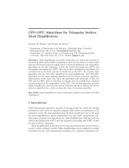
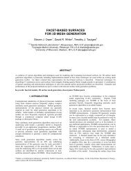
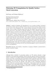
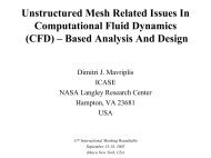
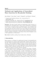
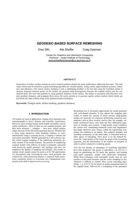
GEODESIC-BASED SURFACE REMESHINGOren Sifri Alla Sheffer Craig GotsmanCenter for Graphics and Geometric ComputingTechnion – Israel Institute of Technology{orensi/sheffa/gotsman@cs.technion.ac.il}ABSTRACTGeneration of surface meshes remains an active research problem despite the many publications addressing this topic. The mainissues which must be treated by a good remeshing algorithm are: element quality, sizing control, approximation accuracy, robustnessand efficiency. One reason surface meshing is such a challenging problem is the fact that using the Euclidean metric tomeasure distances between points on the surface can generate large discrepancies between the original surface and the constructedmesh. We solve this problem by using geodesic distances on the surface. The ability to accurately and efficiently computegeodesic distances, and propagate them across the mesh, permits us to generate quality surface meshes which closely approximatethe input without using costly parameterization techniques.Keywords: Triangle mesh, surface meshing, geodesic distances.1. INTRODUCTION3D models are used in applications ranging from animation andcinematography to heavy industry and scientific visualization.However, most existing surface mesh models can hardly even becalled satisfactory. Most of them are not sampled properly andtheir basic elements — triangles — have poor, almost randomshapes because of the 3D mesh acquisition process. Whether thisis done using interactive solid modeling software or semiautomaticallyusing a scanning device, it remains a tedious anderror-prone procedure. Models generated by CAD software usuallyreflect regular sampling of the underlying parametric domaininstead of the model features. The process of simplifyingscanned models with millions of points is primarily concernedwith preserving model geometry and topology and does notemphasize the quality of sampling and triangles. This results inmeshes which usually cannot be used as-is for 3D applications.An intermediate step, correcting the basic mesh geometry andconnectivity, while preserving features, is required. Such corrections,commonly known as remeshing, are a fundamental componentin the field of digital mesh processing.Remeshing tries to accurately approximate the model geometrywith well-shaped elements. It also adjusts the sampling rateslocally to match the amount of detail present. High-qualitymeshes are necessary for engineers performing numerical computations,such as finite element analysis that, for example, calculatemechanical stress, solve heat and flow differential equationsor simulate such systems. A high-quality mesh conditionsthe system well, eliminating numerical errors and singularitiesthat might otherwise arise. Hence, within the engineering communitythe emphasis is on quality. The computer graphics andmodeling community, on the other hand, is concerned with anotheraspect of remeshing. Their focus is on the tradeoff betweenthe visual quality of the result, the speed of the remeshingoperation, and the optimization of the number of polygons inorder to achieve interactive rendering speeds.Over the last decade, an abundance of remeshing algorithmshave been proposed. One group of algorithms, e.g. [10,11], isbased on partitioning the 3D mesh into patches, and treatingeach patch separately, usually with subdivision techniques.While these techniques yield reasonable results, they are verysensitive to the patch structure, and the vertex sampling (or distribution)is difficult to control. More recent remeshing algorithms,e. g. [2,9,12,14] are based on global parameterization ofthe original mesh, followed by a resampling of the parameter

domain. After this, the new triangulation is “projected” backinto 3D space, resulting in an improved version of the originalmodel. The main drawback of the global parameterization methodsis the sensitivity of the result to the specific parameterizationused. Embedding a non-trivial 3D structure in the parameterplane severely distorts this structure, and important information,which is not specified explicitly, may be lost on the way. Even ifthe parameterization minimizes the metric distortion of the 3Doriginal in some reasonable sense, it is impossible to eliminate itcompletely. Moreover, global parameterization is very slow,usually involving the solution of a large set of (sometimesnonlinear) equations. Because of the size of the system, thissolution may be numerically imprecise, especially in regionswhere the connectivity has bad isoperimetric ratios. These regionscorrespond to protruding extremities in the 3D mesh (e.g.the legs of an animal), and they may be lost in the process. Additionally,2D parameterization requires the surface to be cut toa disk-like topology, both to parameterize closed surfaces orsurfaces with genus higher than zero, and to reduce the parametricdistortion. These cuts introduce visible artifacts in the mesh.The main alternative to global parameterization is to work directlyon the surface. Remeshing algorithms using this approach[2,8,16,18] usually involve difficult, inefficient and limited optimizationsin 3D. For example, Frey and Borouchaki [8] performlocal modifications in the tangent plane. In a subsequentwork, Frey [7] uses a paraboloid to obtain a better approximationof the surface. These complex approximations are extremelyslow and not always robust.The common denominator of all the meshing algorithms is thatthey use Euclidean metrics, in the sense that the distance betweenpoints, even on the surface, is measured as the Euclideandistance between them. Since in most cases we should actuallybe using the geodesic distance, i.e. the distance between thepoints along the surface, this may introduce error culminating indistortion. The Euclidean distance may be considered a goodapproximation to the geodesic distances only at short ranges andin regions of low curvature. Otherwise it is quite different.Nonetheless, the published methods use Euclidean distancesbecause they are much simpler to compute.Assuming a constant sizing function, the vertices of the newmesh should be positioned on the surface such that the distancesalong the surface between close vertices are approximatelyequal. One way of achieving this is to build a "front" of verticeswhich advances across the surface at uniform "velocity" [3,17].The front forms strips of triangles as it advances. The mainproblem with this method is that the front may meet itself, hencesplit and merge as it propagates. This complicates matters significantly,and a number of heuristics are required to control theprocess. The fact that Euclidean distances are employed here aswell results in suboptimal results. Figure 1 shows the result of anadvancing front technique implemented in a commercial package.The loss of high curvature features is a typical artifact. Theresult of applying our method on the same model with similaruniform sizing is shown in Figure 2(e). Due to these difficulties,advancing front techniques are not considered to be very attractive.Figure 1: Horse model (left). Original (right). Advancingfront remesh, produced by an anonymous commercialmesh generator. Note how the details of theears and hooves are lost.1.1 Our ContributionThis work introduces a novel remeshing method which operatesdirectly on the 3D surface in a manner similar to the "advancingfront" methods. So on the one hand, it does not involve anycostly parameterization methods. On the other hand, it avoids allthe pitfalls of the existing advancing front methods. Firstly, ituses geodesic distances instead of Euclidean distances. Secondly,it does not have to deal with major topological changes inthe advancing front. This is achieved by segmenting the meshinto regions such that the treatment of each region is relativelystraightforward. This also allows us to process meshes witharbitrary topologies.2. ALGORITHM OVERVIEWOur mesh generation procedure avoids the need for costly planarparameterization by computing accurate geodesic distances directlyon the surface. The geodesic distances are computed usingthe "fast marching on triangulated domains" technique ofKimmel and Sethian [13]. We provide a brief overview of thetechnique in Section 3.The basic meshing technique we use was first proposed by Adi[1]. It is based on generation of equidistant curves on the surface.An equidistant curve is the locus of all points on the surfaceat some fixed geodesic distance from a given point. Adicomputed such equidistant curves from a single root point on thesurface and then simply triangulated the strips between consecutivecurves.The difficulty with this simple approach, as with the advancingfront techniques, is that equidistant curves may have complextopologies. The saddle regions where a single curve splits intoseveral components can have arbitrary shape (Figure 2(a)).Without special treatment, the mesh in such regions will bothdisobey the sizing requirement and contain badly shaped triangles(Figure 2(b)). Adi did not provide a satisfactory solution tothese problems, hence he was able to generate good meshes onlyfor very simple models. We avoid this pitfall by first segmentingthe surface into regions, such that the distance function is mono-

tone inside each region and therefore does not contain saddlepoints. Once the regions and the equidistant curves inside themare computed, each strip between two adjacent equidistantcurves is meshed using a Voronoi tessellation of vertices distributedon the two curves. The next four sections describe themain components of the algorithm:1. Computation of geodesic distances and equidistant curves.2. Mesh preprocessing.3. Segmentation into regions.4. Triangle generation within each region.The various stages of the algorithm are illustrated in Figures 2and 4.3. COMPUTING GEODESICSThe easy, but inaccurate, way to compute a "geodesic" distancebetween two vertices of a triangle mesh surface is to run a shortest-pathalgorithm on the mesh graph, where the weight associatedwith an edge is its length. Efficient algorithms, such as theDjikstra algorithm [15], can compute these path lengths veryefficiently, but can be shown to produce paths quite differentfrom true geodesic paths. This is because the geodesic path doesnot necessarily pass through the mesh vertices, rather takesshortcuts through edges. See Figures 3(a) and 3(b) for a comparison.In our work we utilize the "fast marching on triangulateddomains" algorithm of Kimmel and Sethian [13]. It computesapproximate geodesic paths between two vertices inO(nlogn) time per path (n is the number of vertices in the mesh).Unfortunately, this algorithm does not always guarantee a correctresult, in particular when the mesh contains triangles withobtuse angles. Kimmel and Sethian offer a solution to this problem,but it is rather complex and not always correct. Alternatively,the problem may be reduced by a preprocessing stepwhich reduces the relative number of obtuse triangles in themesh. The standard way of doing this is to refine the obtusetriangles so that most of the affected area is covered by smaller,but less problematic triangles. This is not guaranteed to removeall obtuse angles, but removing just the worst cases suffices toproduce reasonably accurate geodesic distance computations.Fortunately, obtuse triangles do not occur so frequently, so the(a) (b) (c)(d) (e) (f)Figure 2: The effect of mesh segmentation on geodesic remeshing with uniform sizing of the horse model of Figure1(a). (a) Geodesic curves and zoom on a saddle region. The root vertex is on the back left foot (marked by a star) (b)Resulting mesh with artifacts in saddle regions. (c) Segmented regions. The centers of leaf regions are highlighted bycircles. (d) Geodesic curves formed with two-site distances on segmented mesh. Note that the saddle of (b) hasdisappeared. (e) Resulting mesh with no artifacts. (f) Mesh after post-processing.

algorithm produces quite good results in general, even withoutthese two workarounds, although we employ them both.The fast-marching method can also be adapted to non-uniformgeodesic distances. The input may contain an arbitrary weightper vertex, where larger weights mean that the region surroundingthat vertex is "harder" to pass through. The geodesics thentake this information into account. This is a feature which is veryuseful to us, as we will see later.We use the fast-marching method to compute the equidistantcurves. This is done by computing the geodetic distance fromthe source to all other vertices of the mesh. The equidistantcurve is then formed by connecting linear segments betweenpoints on the edges at a given distance, these too interpolatedlinearly between vertex distances. This approximation is obviouslynot correct when large triangles are involved, since theequidistant curves will be quite different from what they shouldbe. See Figure 3(c); the equidistant curves on a plane are notcircles, as would be expected. Here too, a possible solution,which we adopted, is to refine the mesh to contain many smallertriangles, forcing the algorithm to output more detailed geodeticinformation. Obviously, this increases the computation complexity.(a) (b) (c)Figure 3: Shortest paths between the two yellow vertices.(a) Dijkstra. (b) Geodesic. (c) Equidistant curvesbased on geodesic distances.4. MESH PRE-PROCESSINGOur meshing algorithm supports different sizing requirements ondifferent regions of the mesh. Curvature-based sizing defined foreach vertex is usually used to provide more accurate geometryapproximation. Other per-vertex sizing data, such as those derivedfrom analysis requirements, can be incorporated similarly.This data is sent as input to the fast-marching method, whichconveniently, is able to use it.We approximate the curvature at the mesh vertices using themethod described in [5]. The sizing is then based on a combinationof Gaussian and mean curvature. The relative weight of thetwo components is controlled by the user. In addition the useralso controls the contrast or the gradient of the sizing gradation.This is achieved by transforming the sizing by some polynomialmagnifying function.The required number of triangles determines the desired edgelength in the case of uniform sizing. This in turn determines thedistance between consecutive equidistant curves on the surface.This distance C d is the desired edge length scaled by 3 / 4 (theratio between the height and the side in an equilateral triangle).Now the root vertex for the distance computations is located. Wecompute the two vertices on the surface forming the maximalsurface distance between them (the diameter) and select one ofthem as the root r. The computation of these two vertices is doneusing the following well known iterative procedure [6]:1. Set r to some arbitrary vertex. Set D max to zero.2. Find the farthest vertex t from r. Set D t to the distancebetween r and t.3. If D t > D max , set r := t, D max := D t , and goto 2.This procedure is actually not guaranteed to find the mesh diameter,as it might get stuck in a local minimum, but for reasonablywell-behaved meshes, this is rare. The root vertex r andthe maximal distance D max are used in the following stage tosegment the mesh into regions. Figures 2(a) and 4(b) show theroot vertex and the equidistant curves surrounding it for thehorse and cactus models.5. REGION SEGMENTATIONOnce the root vertex r is found we compute the geodesic distanceD(v) from r to every other vertex v on the mesh. D(v) isthen used to segment the mesh into regions to avoid mesh artifactslike those seen in Figure 2(b). The regions are constructedsuch that each equidistant curve within the region will be wellbehaved.To guarantee this, each region must be a simply connectedregion. See Figures 2(c) and 4(f).The regions form a tree structure containing three types of regionnodes: leaves, interior nodes, and a root. The distinctionbetween different types of regions reflects the properties of thedistance function D. Leaf regions are formed around the maximaof D. Interior regions roughly correspond to the saddle points ofD, and the root region is formed around the root vertex r (theglobal minimum of D). The tree construction algorithm runs intwo stages. First the topological structure of the tree (Figure4(e)) is determined, and then the mesh regions corresponding toeach node are computed (Figure 4(f)).Tree structure construction: The set of vertices L which arethe local maxima of D define the tree leaves (Figure 4(c)). Initiallyeach leaf defines a degenerate tree consisting of a singlenode, producing a forest. A bottom up construction is performedwith groups of trees connected by interior region nodes. Finallyall the trees are joined into a single tree with a single root regionnode.The tree construction uses a front propagation procedure on thesurface starting from the set of leaf vertices L. The front propagationis based on the distance metric D. The fronts emanatingfrom the leaf vertices are propagated so that at each step thevertex with smallest value of D is added to the front of the appropriateleaf l. When two fronts meet at a vertex, an interiorregion node is added to the tree as the parent of the two leaves(Figure 4(d)). The vertex is stored for further processing. Thetwo fronts are merged, and the new front continues to advanceusing the minimal distance D from among its leaves. Whenevertwo fronts meet, interior nodes are created joining the sub-trees(Figure 4(c)). When only one front remains, i.e. all the leaves areconnected into a single tree, the root node is introduced as thecommon parent. At the end of this procedure a region tree

232323111V44V5(a) (b) (c) (d) (e)14235(f) (g) (h) (i) (j) (k)Figure 4: Algorithm stages. (a) Input cactus model. (b) Root vertex (highlighted by star) and curves equidistant fromit. (c)-(e) Computing the region tree structure: (c) Maxima of distance from root. These are leaves of the region tree.(d) Propagating regions around maxima till regions 1 and 2 meet at interior region 4. (e) Continuing propagation ofregions 4 and 3 until they meet at root region 5. (e) Resulting tree structure. (f) Resulting mesh regions. Regions 1, 2and 3 are leaves, region 4 is interior, and region 5 is the root. (g)-(i) Computing equidistant curves within the regions:(g) Propagating equidistant curves down regions 1 and 2. (h) Propagating equidistant curves down region 4. (i) Completeset of strips. (j) Mesh after strip triangulation. (k) Final mesh after smoothing.structure (Figure 4(e)) is defined, but the boundaries of the regionsstill need to be determined.Tree regions construction: The region boundary definitionproceeds yet again bottom up, from the leaves to the root. Whenconsidering a region, the top of the region is defined as:• the center vertex l for a leaf region;• the boundary curve between the region and its children foran interior or root region.The region boundary construction proceeds as follows:While not all the boundaries have been constructed, find an interiornode at which both the following hold:• the top boundary is not defined,• in both of its sub-trees the top boundaries are defined forall the nodes.Note that at the beginning of the procedure all interior nodeswith two leaf children satisfy this condition. Let t 1 and t 2 be thetops of the root nodes of the sub-trees. The vertex v at which thefronts of the sub-trees meet is known from the tree structureconstruction stage above. We now use it to compute the topboundary of the interior node which is the parent of the two subtrees,as follows:• Compute the equidistant curve C at distance D(v) from theroot r. Note that C will contain v.• Find two vertices v 1 and v 2 on C at minimal distance from t 1and t 2 respectively.• Compute the two equidistant curves C 1 and C 2 at distanceC d ⋅⎣D(t 1 ,v 1 )/C d ⎦ from t 1 and at distance C d ⋅⎣D(t 2 ,v 2 )/C d ⎦from t 2 respectively. This distance roundoff makes the distancefrom the tops of the two sub-tree root node regions totheir bottom a multiple of C d . It will result in an even curvedistribution inside the regions at the meshing stage.

• Connect C 1 and C 2 into a “spectacles” shape using theshortest path between them which passes through v. Thisprovides a single loop as the top boundary of the parentnode.The procedure is continued upwards inside the tree until all theregion boundaries are computed. Figure 4(b)-(e) illustrates thisprocedure on the cactus model, resulting in the regions in Figure4(f). Figure 2(c) shows the regions for the horse model. Notethat many leaf patches on the head and legs of the latter are generatedaround minor local maxima. As a result D(l,v)

The example models showcase the method's ability to correctlycapture sock-like shapes such as the animal's legs without requiringglobal parameterization. As is evident in the griffin andfigure eight models, our method does not require any specialtreatment to handle models with genus greater than one. This, inaddition to generating seamless meshes is yet another advantageof this technique over methods which utilize a parameter domain[2,9,12,14]. Our advantage over local methods [7] is in the meshquality (Figure 6), with only a slight penalty in approximationerror in some cases.Both approximation and quality measures are shown in Table 1.The quality is demonstrated by the statistics of the minimal angle.The angles in the inputs are arbitrarily bad, but in most ofthe results, not many angles are less than 30 o and the averageangle is consistently above 50 o . The statistics also include theHausdorff distance from the original model measured using theMetro tool [4]. This is approximately 0.5% of the bounding boxdiagonal for most models, which is quite negligible. The superiorityof using geodesic distance based advancing front instead ofclassical advancing front techniques in terms of approximation isclearly demonstrated by the horse meshes in Figure 1.Input Result Con InputResult Apprsize size tras Angles (deg.) Angles (deg.) Error(#ver) (#ver) tMin %

[9] X. Gu, S.J. Gortler and H. Hoppe, Geometry images, ACMTransactions on Graphics. Special issue for SIGGRAPHconference, 21(3), (2002), pp. 355–361.[10] I. Guskov, K. Vidimce, W. Sweldens, and P. Schroeder,Normal meshes, Computer Graphics. SIGGRAPH 2000Proceedings, (2000), pp. 95–102.[11] H. Hoppe, T. DeRose, T. Duchamp, J. McDonald and W.Stuetzle, Mesh optimization, Computer Graphics. SIG-GRAPH ’93 Proceedings, 27 (1993), pp. 19–26.[12] K. Hormann, U. Labsik and G. Greiner, Remeshing triangulatedsurfaces with optimal parameterizations, Computer-Aided Design, 33 (2001), pp. 779–788.[13] R. Kimmel and J.A. Sethian. Computing geodesic paths onmanifolds. Proceedings of National Academy of Sciences,95(15) (1998), pp. 8431-8435.[14] A. Sheffer and E. de Sturler. Parameterization of facetedsurfaces for meshing using angle based flattening, Engineeringwith Computers, 17(3), (2001), pp. 326-337.[15] S. Skiena. The algorithm design manual. Springer, 2000.[16] V. Surazhsky and C. Gotsman. Explicit surface remeshing.Proceedings of the ACM/Eurographics Symposium on GeometryProcessing (2003), pp. 17-27.[17] J.R. Tristano, S.J. Owen and S.A. Canann. Advancing frontsurface mesh generation in parametric space using a Riemanniansurface definition. Proceedings of the 7th InternationalMeshing Roundtable, 1998.[18] G. Turk. Re-tiling polygonal surfaces. Computer Graphics26:2, SIGGRAPH 1992 Proceedings, pp. 55-64.

VenusGearFigure EightDinoFigure 7: Remeshes. Left: Input mesh. Middle: Remesh. Right: Zoom on remesh (except the Venus model which has adifferent contrast).

CamelGriffinFootFigure 7 (cont.): Remeshes. Left column is the input mesh. Middle is the remesh and right is a zoom.

(a) (b) (c) (d)Figure 8: The effect of segmentation. The statistics of the results appear in Table 1. (a) Input tree mesh. (b) Remeshwithout segmentation. (c) Segments generated by our algorithm. (d) Remesh with segmentation.